The roadmap for unification in galaxy group selection:. I. A search for extended X-ray emission in the CNOC2 survey.^∗

Abstract

X-ray properties of galaxy groups can unlock some of the most challenging research topics in modern extragalactic astronomy: the growth of structure and its influence on galaxy formation. Only with the advent of the Chandra and XMM facilities have X-ray observations reached the depths required to address these questions in a satisfactory manner. Here we present an X-ray imaging study of two patches from the CNOC2 spectroscopic galaxy survey using combined Chandra and XMM data. A state of the art extended source finding algorithm has been applied, and the resultant source catalog, including redshifts from a spectroscopic follow-up program, is presented. The total number of spectroscopically identified groups is 25 spanning a redshift range 0.04–0.79. Approximately 50% of CNOC2 spectroscopically selected groups in the deeper X-ray (RA14h) field are likely X-ray detections, compared to 20% in the shallower (RA21h) field. Statistical modeling shows that this is consistent with expectations, assuming an expected evolution of the L_X–M relation. A significant detection of a stacked shear signal for both spectroscopic and X-ray groups indicates that both samples contain real groups of about the expected mass. We conclude that the current area and depth of X-ray and spectroscopic facilities provide a unique window of opportunity at $z\sim 0.4$ to test the X-ray appearance of galaxy groups selected in various ways. There is at present no evidence that the correlation between X-ray luminosity and velocity dispersion evolves significantly with redshift, which implies that catalogs based on either method can be fairly compared and modeled.

1. Introduction

Groups of galaxies constitute the most common galaxy associations, containing as much as 50-70% of the galaxy population at the present day (Geller & Huchra 1983; Eke et al. 2005). Given that most galaxies will encounter the group environment during their lifetime, an understanding of groups is vital to understanding galaxy evolution in general. The characteristic depth of the potential wells of groups is similar to those of individual galaxies, and the velocities of member galaxies are only a few hundred km/s. Under these circumstances, galaxies interact strongly with one another and also with the larger scale environment. Recent simulation work suggests that strangulation and ram-pressure stripping may quench star formation in galaxies inhabiting groups with a significant intragroup medium component (Kawata & Mulchaey 2008; McCarthy et al. 2008). Hence, not only are groups the most common environment for galaxies, but also they provide an environment which may have a strong effect on galaxy properties.

Perhaps the best way to understand the role the group environment plays in galaxy evolution is to study the galaxy populations in groups over a range of cosmic time. Historically, such studies have been limited because it has been difficult to define group samples out to even moderate redshifts. This situation is rapidly changing, however. The recent completion of very large redshift surveys now allows large group samples to be kinematically-defined out to z $\sim$ 1 (Carlberg et al. 2001; Gerke et al. 2005). The current generation of X-ray telescopes also allows identification of X-ray groups over a similar redshift interval (Willis et al. 2005; Finoguenov et al. 2007).

Follow-up studies of these group samples suggest that indeed there has been considerable evolution in the group environment since z $\sim$ 1. In spectroscopically-selected groups, there is evidence for a significant drop in the fraction of strongly star-forming galaxies over the last few billion years (Wilman et al. 2005b). This process is further accompanied by an apparent increase in the population of S0 galaxies (Wilman et al. 2009). Recent studies show that, unlike their low redshift counterparts, many X-ray luminous groups at intermediate redshift lack a dominant central galaxy (Mulchaey et al. 2006; Jeltema et al. 2006, 2007). This implies that even the most massive groups at intermediate redshifts are still in the process of evolving.

Despite these first efforts to study groups over a range of cosmic time, a coherent picture for the role they play in galaxy evolution has proved elusive. One of the reasons for this is that groups are a very heterogeneous class of objects: they span a wide range of dynamical states from objects just in the process of collapsing for the first time (like the Local Group) to fully virialized systems with properties much like galaxy clusters (e.g., Zabludoff & Mulchaey 1998; Rasmussen et al. 2006). Unfortunately, none of the aforementioned studies have included groups across this complete range of dynamical states. This is largely because of selection effects: groups selected to be X-ray luminous are biased toward more massive, evolved and relaxed systems, while spectroscopically-selected samples are dominated by small associations of a few galaxies that would normally be undetectable in X-ray emission. In addition, few studies have had both good membership information (which requires extensive spectroscopic programs) and X-ray data (the best indicator of a group’s dynamical state) and both of these are needed to obtain a comprehensive understanding of the group environment.

Unfortunately, most groups are not X-ray luminous and therefore relatively long X-ray observations are required to study these objects. For this reason, most studies have been restricted to groups that are a priori known to be X-ray bright. Much less is known about the X-ray properties of the more common systems that dominate spectroscopic group catalogs. In fact, the fraction of spectroscopically-selected groups that contain a significant X-ray emitting intragroup medium is still very poorly constrained (Mulchaey 2000). XMM-Newton studies of a few spectroscopically-selected groups suggest their properties may be quite different from those of X-ray luminous systems (Rasmussen et al. 2006).

An additional problem with studying groups is that it is difficult to accurately determine the masses of these systems. One promising technique is to use weak lensing measurements, which has been extensively used as a tool for measuring the masses and dark matter profiles of galaxy clusters (e.g., Fahlman et al. 1994; Luppino & Kaiser 1997; Hoekstra et al. 1998; Clowe et al. 2006; Kubo et al. 2007) and the statistical studies of galaxy-sized halos (Brainerd et al. 1996; Hudson et al. 1998; Hoekstra et al. 2005; Mandelbaum et al. 2006b; Parker et al. 2007). This technique can also be employed for studies of galaxy groups (Hoekstra et al. 2001; Parker et al. 2005; Mandelbaum et al. 2006b) though few studies have been carried out, largely due to a lack of large samples of galaxy groups at intermediate redshifts. Unlike rich galaxy clusters, individual galaxy groups do not produce a measurable weak lensing signal and therefore the signal from multiple groups must be stacked, much like the techniques employed in galaxy-galaxy lensing.

Our approach to these problems is to perform a deep X-ray survey in an area of the sky where an extensive spectroscopic survey, and deep optical imaging, has been completed. Our X-ray observations have been designed to guarantee the detection of X-ray groups down to low X-ray luminosities and out to intermediate redshifts where the spectroscopic coverage is complete enough to allow groups to be spectroscopically identified. By combining the optical and X-ray data, we can select groups over the full range of dynamical states. Furthermore, by restricting our analysis to intermediate redshifts, we can take advantage of the deep imaging to estimate weak lensing masses for these groups.

The paper is structured as follows: in §2 we recall the construction of the sample of spectroscopic groups; in §3 we describe the archival and our own XMM-Newton and Chandra observations of the field and present the details of the image processing technique and selection of extended X-ray systems; an ongoing, dedicated spectroscopic follow-up program is outlined in §4 and the catalog of X-ray systems which could be unambiguously identified is introduced in §5. In §6 we describe the stacked weak lensing analysis and provide the characteristics of various group samples and in §7 we discuss which spectroscopic groups are identified in X-rays. We summarize our results in §8. The goal of this paper is to present the extended X-ray source catalog and provide a template for comparison with the spectroscopic group catalog. Results presented here are part of an ongoing program: additional spectroscopic, deeper X-ray and multiwavelength imaging data will provide improved statistics and diagnostics for future papers.

All through this paper, we shall adopt a “concordance” cosmological model, with $H_{o}=72$ km s^-1 Mpc^-1, $\Omega_{M}=0.25$, $\Omega_{\Lambda}=0.75$, and — unless specified — quote all X-ray fluxes in the [0.5-2] keV band and rest-frame luminosities in the [0.1-2.4] keV band, provide the confidence intervals at the 68% level and evaluate the enclosed density in a definition for masses and radii in respect to the critical density.

2. CNOC2 Survey and Groups

The second Canadian Network for Observational Cosmology Field Galaxy Redshift Survey (CNOC2) is one of the few completed surveys with spectroscopic and photometric data for a large, well-defined sample of galaxies, obtained for the purpose of studying the evolution of galaxy clustering (Yee et al. 2000). CNOC2 is magnitude limited down to $\rm\,R_{C}\sim 23.2$ in photometry and totals $\sim$1.5 ^∘ within four separate patches on the sky. Spectroscopic redshifts, mainly in the range 0.1$\leq z\leq$0.55 exist for a large and unbiased sample of $\rm\,R_{C}\lesssim 21.5$ galaxies (Yee et al. 2000). Galaxy groups have been identified by applying a friends of friends algorithm to detect significant overdensities in redshift space, with parameters tuned to pick up virialized systems (Carlberg et al. 2001): in practice this means that group selection is tuned such that at least three galaxies with CNOC2 redshifts are clustered tightly enough that they appear at least 200 times overdense with respect to the critical density. The resulting sample contains over 200 systems in $\sim$1.5 ^∘ spanning a broad range of dynamical states.

To study the evolution of galaxies in the group environment, we undertook an extensive follow-up program of a subset of these groups using the Magellan 6.5-m telescopes in Chile (Wilman et al. 2005a), HST, Spitzer, Chandra, XMM-Newton and GALEX among other facilities. This extensive dataset allows us to study the properties of the galaxies and the groups in detail. These data provide ample evidence for significant changes in the star formation rates and morphological composition of groups galaxies over the last 5 billion years, and differences from the field population (Wilman et al. 2005a,b, 2008, 2009; Balogh et al. 2007, 2009; McGee et al. 2008).

3. X-ray data and methods for extended emission search

X-ray data have been obtained for two of the four CNOC2 patches described in §2 (the RA14h and RA21h patches). Each of these patches has been observed on several occasions with both XMM-Newton and Chandra. The XMM-Newton OBSIDs for the RA14h patch are 0148520101, 0148520301, and 0149010201, while the Chandra OBSIDs for this patch are 5032, 5033 and 5034. The XMM-Newton OBSIDs for the RA21h patch are 0404190101 and 0404190201 and the Chandra OBSID for this patch is 6791.

To increase our sensitivity to low level X-ray emission, our analysis is performed on X-ray mosaics made from the co-addition of the XMM-Newton and Chandra data. Throughout this paper, we list the effective exposure times in each field in units of the equivalent Chandra exposure that would be required to reach the observed sensitivity in the 0.5–2 keV band for a 2 keV thermal diffuse emission at z=0.2. The maximum effective exposure times in these units are 348 ksec in the RA21h patch and 469 ksec in the RA14h patch. We note, that in calculating the properties of systems with a known redshift, we self-consistently re-estimate the effective sensitivity, accounting for the measured redshift and expected temperature (using $L_{X}$; see Finoguenov et al. 2007). In Fig.1 we present the exposure map for both patches. The primary differences between the X-ray coverage of the two fields is that the depth in the RA14h patch is more uniform, while most of the RA21h area has an effective exposure much less than the maximum (most of the field has an effective exposure time of $\sim$ 100 ksec or less).

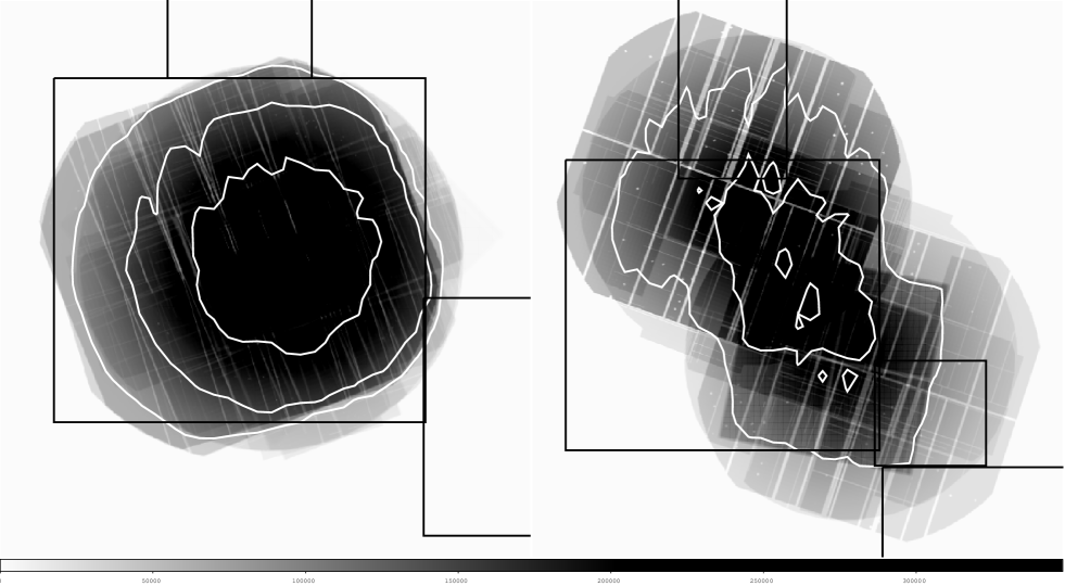
Figure 1.— Exposure maps of RA14h (left) and RA21h (right) patch of CNOC2. Co-added XMM and Chandra exposures are shown. The contours (white) indicate the achieved level of effective 100, 200 and 300 ksec Chandra depth in the 0.5–2 keV band for a 2 keV source at z=0.2 (see text). The total area covered by X-ray observations is 0.2 and 0.3 square degrees for the RA14h and RA21h fields, respectively. The black boxes show the boundary of the CNOC2 redshift survey.

3.1. XMM routine for point source removal

In making the X-ray mosaic, we use a new procedure, which has now been applied to several deep X-ray surveys (COSMOS, SXDF, LH, CDFS, CDFN, PISCES fields). A direct comparison between XMM and Chandra catalogs, possible in CDFS&N, yields 80-90% agreement in the source catalogs, with some residual contamination due to alignments of AGNs that were unresolved in the XMM dataset but were resolved with Chandra (Finoguenov et al. in prep.). The XMM data reduction was done using XMMSAS version 6.5 (Watson et al. 2001; Kirsch et al. 2004; Saxton et al. 2005). In addition to the standard processing, we perform a more conservative removal of time intervals affected by solar flares, following the procedure described in Zhang et al. (2004) (see Finoguenov et al. 2007 for details). In order to increase our sensitivity to extended, low surface brightness features, in addition to adopting the background subtraction procedure of Finoguenov et al. (2007), we also removed all hot MOS chips. From our careful monitoring of the quality of the background subtraction, we confirm the findings of Snowden et al. (2008) that episodically one chip in either MOS1 or MOS2 exhibits a distinctly higher background below 1 keV. This effect is particularly problematic for recent XMM observations.

After the background has been estimated and subtracted for each observation and each instrument separately, we produce the final mosaic of cleaned images and correct it with a mosaic of the exposure maps. In this process, we also account for the differences in sensitivity between the pn & MOS detectors.

As we are interested in identifying extended X-ray sources, adequate point source removal is vital. The formal confusion limit for the XMM PSF precludes using large scales for source detection at exposures exceeding 100 ksec. However, since the shape of PSF is not Gaussian, the information on large scales can be restored using the detection of point sources on small scales and subsequent modeling of the point source flux. To illustrate the point, since the observed image is a convolution of the original image and the instrument PSF, we present the arguments in the Fourier space, where the convolution is a mere multiplication of the Fourier transforms. As the Fourier transform of a Gaussian is also a Gaussian, this very effectively suppresses any information on scales below the width of the distribution. The XMM PSF can be approximated by a sum of 3 Gaussians, so a convolution with such a function is a sum of 3 convolutions, proving that the information is still retained on scales larger than the width of the core of PSF ($5^{\prime\prime}$). This defines the theoretical lower limit on recovering the information content in XMM images.

It is also obvious that the removal of point source flux has to be done prior to examining the confused spatial scales. To accommodate this, we introduced such a new process to identify the point sources and to remove their flux. The procedure adopts a symmetric model for the XMM PSF and uses the calibrations of Ghizzardi & Molendi (2002, see also Ferrando et al. 2003). There are three steps of the flux removal, which are wavelet-specific, and their goal is to achieve a correct flux estimate for each detected point source. The wavelet decomposition we employ is both a spatial and a significance filter, so flux is stored and subtracted from the input image, before applying the next spatial scale filtering, only if its significance is larger than some threshold (Vikhlinin et al. 1998). As a result, in the wavelet decomposition the flux attributed to each spatial scale varies: as the significance of the source increases, more flux is attributed to smaller scales. A simplified procedure would result in either underestimation of flux pollution from the faint sources or in the overestimation of the pollution from the strong sources. To properly subtract the PSF-induced contribution of small-scales to large-scale features, we perform three reconstructions of the small scales, using the detection thresholds of 100, 30 and 4 $\sigma$. The $4\sigma$ image receives the full weight according to PSF models and the other two reconstructions are subtracted from it with proper weights, which are defined by both the XMM PSF on small scales and properties of the wavelet transformation. A similar and even better result can be obtained by fitting the PSF to the positions of the sources, which we hope to include in future analysis. The XMM PSF model describing the detections on small scales also predicts the flux on large scales. As discussed in Finoguenov et al. (2007), our selection of spatial scales is done to reduce the variation of this prediction with off-axis angle and greatly simplify the procedure of point source flux removal. To subtract the expected flux spread from small to large scales, we convolved the point source image reconstructed above with Gaussians of width 16, 32 and 64 arcseconds, weighted according to the observed PSF and then subtracted this from the image together with the wavelet reconstruction on the small scales. To account for deviations between the symmetric PSF model and a two-dimensional PSF characterization, we add 5% systematic error associated with our model on the 16 and 32 arcsecond scales and 200% systematic error associated with our model on the 64 arcsecond scale. The systematic errors correspond to differences occurring at the edge of the field of view. Using XMMSAS detections of point sources in the Lockman Hole, the model XMM images of point sources in that field have been reconstructed (Brunner et al. 2008). We run our procedure on these randomized images detecting no residual extended emission.

Figure 2.— Signal-to-noise ratio of the point-source removed X-ray images in the 0.5–2 keV energy range of the RA14h (left) and the RA21h (right) CNOC2 patches. The gray scale indicates the significance per $32^{\prime\prime}$ beam starting at 1 $\sigma$ (light gray). Black color indicates a significance in excess of 7 sigma. Ellipses indicate the position and the size of the flux extraction regions used to estimate the properties of identified systems. In addition to the sources detected in the final wavelet reconstruction, 6 low significance X-ray sources from Tab.1 are shown for completeness. Some of the high-significance X-ray peaks are still to be spectroscopically identified.

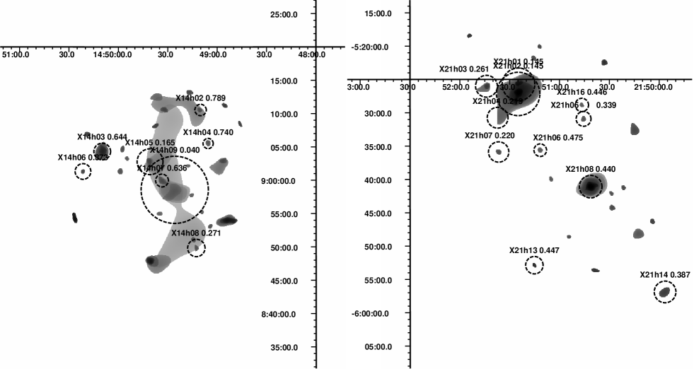
Figure 3.— Wavelet-reconstruction of the point-source removed X-ray image of the RA14h (left) and the RA21h (right) CNOC2 patches on spatial scales from 32^′′ to 256^′′. The units of the image are ergs s^-1 cm^-2 arcmin^-2 and the logarithmic range shown is from -16 to -13 (from light gray to black). Circles indicate the spectroscopically identified X-ray systems with radii of the circle showing the $R_{500}(\approx 0.6R_{200}$). In most cases the emission covers only the core of the detected systems. Some of the high-significance X-ray peaks are still to be spectroscopically identified.

3.2. Chandra data reduction

Initial Chandra data reduction was performed using standard reduction procedures of CIAO version 3.4. In this work we use the available Chandra observations of the CNOC2 fields to further improve the sensitivity toward the detection of extended X-ray emission. Since we use the $32^{\prime\prime}$ and $64^{\prime\prime}$ scales to search for extended emission with XMM, we similarly removed the emission on smaller spatial scales from Chandra data. Large scales considered for extended source detection allowed us to use the full Chandra field for this work. We removed point sources from the Chandra data using the following procedure. For Chandra, the on-axis scattering of point source flux into $32^{\prime\prime}$ scales is negligible, while it becomes important at off-axis angles exceeding $3^{\prime}$. Our simplified point source removal is based on the PSF model which shows that once the scales of $8^{\prime\prime}$ and $16^{\prime\prime}$ are polluted, so are the larger scales. Residual variations in the off-axis behavior of the Chandra PSF are treated as systematic errors in our model. In summary, in addition to the removal of point source flux detected on scales of 1, 2, 4, 8 and 16 arcseconds, we use the emission detected at scales of $8^{\prime\prime}$ and $16^{\prime\prime}$ to predict and subtract the effect of the Chandra PSF, important for off-axis angles exceeding $3^{\prime}$. We added in quadrature a 20% systematic error associated with this model to the error budget.

3.3. Combined X-ray imaging

After instrument–specific background and point source removal, the residual images were co-added, taking into account the difference in the sensitivity of each instrument to produce a joint exposure map. Specifically, the Chandra ACIS-I exposure is taken as it is, each XMM EPIC MOS exposure is counted as equal to Chandra exposure, and the XMM EPIC pn exposure is multiplied by 3.6 times the read-out time correction (0.93–0.98 depending on the read-out mode).

The resulting signal-to-noise images are shown in Fig.2, together with the location of identified systems and the flux extraction regions. To detect the sources we run a wavelet detection at $32^{\prime\prime}$ and $64^{\prime\prime}$ spatial scales, similar to the procedure outlined in Finoguenov et al. (2007). The total number of detections in the RA14h and RA21h patches is 27 and 23, respectively. This corresponds to a source surface density of 135 and 75 per square degree in the two fields, respectively.

The refined procedure of point source flux removal has allowed us to better associate the peak of the X-ray emission with the center of the group. The formal positional uncertainty is of order of $10^{\prime\prime}$, although it can reach $30^{\prime\prime}$ for systems of low statistical significance due to X-ray flux contribution from sources under the detection threshold. The sources flux is measured from the residual image after the background and point sources have been subtracted off. This means that the estimate of flux signal to noise ratio is not the same as the significance of the source detection (estimated using the wavelet image).

4. Additional Optical Spectroscopy

The original CNOC2 survey (Yee et al. 2000) has only a $\sim 30$% sampling rate, as well as a significant spatial variation in spectroscopic completeness. Wilman et al. (2005a) improved the completeness in the regions around a subset of spectroscopically defined groups from Carlberg et al. (2001). However, by definition this was in regions where the completeness was already high enough to find the group in redshift space. Many of the X-ray detected systems therefore exist in regions of highly incomplete spectroscopy, such that it is impossible to determine the group redshift from the existing spectroscopy. Therefore, to determine the redshifts of the X-ray detected systems, we have obtained additional spectroscopy with the VLT and Magellan telescopes. This substantially improves the sampling rate in regions of X-ray emission, increasing the number of group identifications and known membership. The spectroscopic data and group membership will be described in full by Connelly et al. (in prep.), but a brief discussion of new redshift measurements is provided here.

The VLT observations were conducted with FORS2 over the course of three visitor mode observing runs in 2007-2008, with corresponding run IDs of 080.A-0427(D) (0.6 night, Oct 5 2007), 080.A-0427(B) (two half nights starting Mar 1, 2008) and 081.A-0103(B) (two half nights starting Aug 24, 2008). A total of 21 MXU (multi-object) masks (6.8′ $\times$ 6.8′ FOV) were observed. Observations were obtained in both the RA14h and RA21h fields, and were designed to maximize the number of extended X-ray sources targeted. Slits were placed on galaxies with unknown redshifts, prioritizing galaxies close to the X-ray centers and with magnitudes $R_{C}\lesssim 22.0$, although fainter and more distant galaxies were used to fill the masks. The spectral set-up of the observation used the GRIS300V grism and GG375 filter resulting in an effective wavelength range of $\sim 430-700$ nm. A slit width of $1^{\prime\prime}$ was used for all objects. The total integration time per mask was approximately 1 hr. Chip images from consecutive mask exposures were co-added using the IRAF imcombine tool with cosmic-ray rejection applied. The data reduction was performed with the most recent version of the standard FORS pipeline which performs bias correction, flat-fielding, correction for optical distortions, and wavelength calibration (Appenzeller et al. 1998). The pipeline also detects and extracts individual object spectra. Finally, galaxy redshifts were derived manually using the emission lines where available, or the H and K Calcium lines and the G-band feature for absorption redshifts. To date, we have measured redshifts for 364 (312 with high quality) objects from the FORS2 data. This focused on galaxies in the cores of X-ray systems, measuring enough redshifts to be confident of the group redshift. Data reduction of a complete FORS2 dataset is ongoing and further results will be presented by Connelly et al. (in prep).

We also obtained two multi-object masks of the RA14h field using the IMACS instrument on the Baade/Magellan I telescope in July 17-18, 2007. The IMACS observations were taken with a grism of 200 lines mm^-1, giving a wavelength range of $\sim$ 5000–9500Å and a dispersion of 2.0 Å pixel^-1. A slit width of $1^{\prime\prime}$ was used. The exposure time was 2 hour for both masks. The IMACS data were reduced using the COSMOS data reduction package. First, overscan regions of the CCDs were used to measure and subtract the bias level. Domeflat exposures taken during the night were used to flat-field the data. Sky subtraction was performed using the method outlined in Kelson (2003). Wavelength calibrations were determined from HeNeAr arc exposures. Redshifts were measured by cross-correlating the IMACS spectra with SDSS galaxy templates. We measured a total of 57 new redshifts from the IMACS data.

5. A catalog of identified X-ray groups

Table 1Current status of the spectroscopic follow-up of X-ray extended sources.

ID	IAU name	R.A	Decl.	z	$n_{z}$	flux $10^{-14}$	L0.1-2.4keV	M200	$R_{200}$
	CNOC2XGG J	Eq.2000				ergs cm-2 s-1	$10^{42}$ ergs s-1	$10^{13}$ M⊙	$\prime$	optical ID
X14h01a	144949+0910.9	222.45584	+9.18167	$0.132\pm 0.002$	5	0.95$\pm$0.31	0.66$\pm$0.21	1.68$\pm$0.33	3.76
X14h02	144910+0910.5	222.29202	+9.17579	$0.789\pm 0.003$	4	0.27$\pm$0.07	14.31$\pm$3.56	6.94$\pm$1.06	1.85
X14h03	145009+0904.3	222.54075	+9.07188	$0.644\pm 0.001$	9	1.24$\pm$0.13	36.15$\pm$3.83	14.32$\pm$0.95	2.57
X14h04	144905+0905.5	222.27293	+9.09198	$0.740\pm 0.003$	4	0.14$\pm$0.05	6.42$\pm$2.39	4.35$\pm$0.98	1.63
X14h05	144940+0902.7	222.41983	+9.04645	$0.165\pm 0.001$	6	0.89$\pm$0.15	1.01$\pm$0.17	2.16$\pm$0.23	3.38	1
X14h06	145021+0901.3	222.58939	+9.02196	$0.373\pm 0.002$	6	0.39$\pm$0.13	2.93$\pm$0.98	3.63$\pm$0.73	2.20	28
X14h07	144933+0859.9	222.38956	+8.99939	$0.636\pm 0.004$	3	0.32$\pm$0.05	10.02$\pm$1.89	6.34$\pm$0.74	1.97
X14h08	144912+0849.8	222.30276	+8.83071	$0.271\pm 0.001$	10	0.35$\pm$0.10	1.26$\pm$0.36	2.30$\pm$0.40	2.35	11
X14h09	144925+0858.5	222.35742	+8.97616	$0.040\pm 0.001$	5	2.68$\pm$0.35	0.16$\pm$0.02	0.73$\pm$0.06	8.49
X21h01	215124$-$0525.6	327.85410	$-$5.42783	$0.146\pm 0.001$	11	2.10$\pm$0.38	1.72$\pm$0.31	3.08$\pm$0.34	4.25
X21h02	215124$-$0527.5	327.85155	$-$5.45853	$0.145\pm 0.001$	19	7.63$\pm$0.29	6.50$\pm$0.25	7.21$\pm$0.17	5.64	104
X21h03b	215143$-$0526.0	327.93324	$-$5.43371	$0.262\pm 0.001$	8	0.95$\pm$0.18	3.14$\pm$0.58	4.15$\pm$0.48	2.94
X21h04	215135$-$0530.4	327.89632	$-$5.50686	$0.219\pm 0.001$	12	0.57$\pm$0.12	1.21$\pm$0.26	2.34$\pm$0.31	2.77	117
X21h05	215045$-$0530.9	327.68966	$-$5.51535	$0.338\pm 0.002$	6	0.25$\pm$0.08	1.52$\pm$0.48	2.45$\pm$0.47	2.05
X21h06	215111$-$0535.6	327.79834	$-$5.59362	$0.474\pm 0.002$	6	0.20$\pm$0.06	2.83$\pm$0.87	3.25$\pm$0.61	1.83
X21h07	215136$-$0535.8	327.90274	$-$5.59811	$0.220\pm 0.001$	12	0.51$\pm$0.14	1.10$\pm$0.31	2.20$\pm$0.37	2.71
X21h08	215041$-$0541.0	327.67186	$-$5.68486	$0.439\pm 0.001$	30	2.82$\pm$0.13	31.63$\pm$1.50	15.72$\pm$0.47	3.23	138
X21h09a	215144$-$0540.3	327.93620	$-$5.67284	$0.734\pm 0.004$	3	0.17$\pm$0.08	7.81$\pm$3.66	4.96$\pm$1.38	1.70
X21h10a	215026$-$0546.2	327.60980	$-$5.77096	$0.392\pm 0.001$	11	0.22$\pm$0.10	1.86$\pm$0.81	2.67$\pm$0.70	1.93
X21h11a	215115$-$0548.0	327.81629	$-$5.80110	$0.567\pm 0.001$	9	0.18$\pm$0.09	4.03$\pm$2.04	3.76$\pm$1.16	1.75
X21h12a	215111$-$0548.5	327.79831	$-$5.80904	$0.143\pm 0.002$	5	0.13$\pm$0.29	0.12$\pm$0.28	0.57$\pm$0.64	2.45
X21h13	215115$-$0552.8	327.81317	$-$5.88123	$0.447\pm 0.002$	6	0.82$\pm$0.29	10.01$\pm$3.56	7.48$\pm$1.62	2.50
X21h14	214956$-$0556.8	327.48498	$-$5.94811	$0.388\pm 0.002$	4	1.86$\pm$0.46	15.46$\pm$3.79	10.40$\pm$1.57	3.05
X21h15a	215202$-$0533.9	328.01069	$-$5.56647	$0.458\pm 0.003$	4	0.18$\pm$0.16	2.41$\pm$2.16	2.98$\pm$1.51	1.81
X21h16	215046$-$0528.8	327.69397	$-$5.48061	$0.445\pm 0.001$	12	0.23$\pm$0.07	2.89$\pm$0.85	3.38$\pm$0.61	1.92

^a – not in the final X-ray catalog, not included in statistical tests.
^b – outside CNOC2 spectroscopic survey

X-ray group redshifts are identified where at least three consistent galaxy redshifts (CNOC2 $+$ preliminary FORS2 and IMACS catalog) lie within the observed extent of X-ray emission ($\sim$0.3$\times R_{200}$). In many cases, the clustering of galaxies in both redshift and projected spatial coordinates is obvious. In some cases a brightest group galaxy (BGG) clearly exists near the X-ray center, but this is not required for group identification. In Tab. 1, we list the 25 X-ray sources associated with spectroscopically confirmed groups. This list includes 6 groups, which were detected at an earlier stage of detection routine development. The flux from these sources is highly uncertain because of systematic uncertainties in the PSF subtraction. We also checked that, except for the X21h09 group, the other 5 groups are still detected with the adopted version of the detection routine, when the threshold for source detection is lowered to 2 sigma. These sources cannot be used in statistical tests, but since their identification has been successful, they provide an example of faintest X-ray groups and the data in Tab. 1 can be used to access their parameters. The final wavelet reconstruction of the point-source removed X-ray image in the 0.5–2 keV band and the 19 spectroscopically identified high-significance peaks are shown in Fig.3.

Total flux in the 0.5–2 keV band is estimated by extrapolating the surface brightness to $R_{500}\sim 0.6R_{200}$ following the model prescription of Finoguenov et al. (2007). Rest-frame luminosity in the 0.1–2.4 keV band is estimated (Finoguenov et al. 2007; Leauthaud et al. 2009) and the total group mass within the estimated $R_{200}$, $M_{200}$, is computed following the $z\sim 0.25$ relation from Rykoff et al. (2008) and assuming standard evolution of scaling relations: $M_{200}E_{z}=f(L_{X}E_{z}^{-1})$, where $E_{z}=(\Omega_{M}(1+z)^{3}+\Omega_{\Lambda})^{1/2}$. The assumed scaling relations for systems of similar mass and redshift have been verified using a weak lensing calibration of X-ray groups in the COSMOS survey (Leauthaud et al. 2009).

The total number of galaxies within $R_{200}$ and $|\Delta z|<0.007(1+z)$ is computed, $n_{z}$. Such selection is relatively loose and will include interlopers, and is done as a preliminary step before applying sigma clipping. Group membership allocation will improve as more redshifts are measured, also providing a better estimate of velocity dispersion and rejection of outliers. At this preliminary stage the measurement of $n_{z}$ reinforces the existence of overdensities at the position and redshift of X-ray groups. Tab. 1 provides cluster identification number (column 1); IAU name (2); R.A. and Decl. of a global center of the extended X-ray emission for Equinox J2000.0 (3 & 4); spectroscopic redshift (5); the number of member galaxies inside $R_{200}$, $n_{z}$ before any sigma-clipping (6); the total flux in the 0.5–2 keV band (7); rest-frame luminosity in the 0.1–2.4 keV band (8); estimated group total mass, $M_{200}$ (9) and the corresponding $R_{200}$ (10). Uncertainties are quoted at the 68% confidence level and do not include the scatter in scaling relations. The final column (11) lists the group number from the spectroscopically selected group catalog of Carlberg et al. where there is a confident match with the X-ray detected system. The X-ray system X14h09 is identified with a bright early-type galaxy at a $z=0.04$: other than spatial coincidence, the very large X-ray extent argues in favor of a low redshift source. Four satellite galaxies within the estimated $R_{200}$ support this hypothesis. However it is likely that emission from spectroscopic group 38 at $z=0.511$ is confused with this foreground system (see §7).

6. Lensing

A weak lensing analysis of a large sample of CNOC2 spectroscopically selected groups has been carried out based on deep CFHT and KPNO 4-m data as described in Parker et al. (2005). High quality R- and I-band data were used to measure the shapes of faint background galaxies. The analysis for each of the 4 CNOC2 fields was based on single-band photometry, so the redshifts for the background sources had to be estimated based on the N(z) distribution from the Hubble Deep Field (Fernández-Soto et al. 1999). Without accurate redshifts for the background sources there could be some contamination in the source catalogs from faint group members. However, we do not find an excess source density around the groups, compared with the field, which suggests that the level of this contamination is small relative to other uncertainties.

In order to compare the weak lensing properties of the spectroscopically and X-ray selected groups the tangential shear signal was recomputed for spectroscopically selected groups within the 14 and 21 hour CNOC2 fields, as well as the area within those two fields overlapping with the region observed at X-rays. The source catalogs used in this analysis are identical to those used in Parker et al. (2005) and have been thoroughly tested for systematics. The stacked weak lensing results are presented in Fig.4a and Tab.2. The tangential shear for a sample of group lenses can be used to calculate the ensemble-averaged velocity dispersion, assuming an isothermal sphere density profile, as follows

$$\gamma_{T}=\frac{\theta_{E}}{2\theta}=\frac{2\pi\sigma^{2}}{c^{2}\theta}\frac{D_{LS}}{D_{S}}$$ (1)

where $\theta_{E}$ is the Einstein radius of the lenses, $\theta$ is the angular distance from the group center, $D_{LS}$ is the angular diameter distance between the lenses and sources, and $D_{S}$ is the angular diameter distance to the sources. The best fitting isothermal sphere yields a velocity dispersion of 228$\pm$137 km s^-1 for all spectroscopically selected groups in the two patches and 260$\pm 110$ km s^-1 for those within the region of the survey covered by X-ray data. The sample of all X-ray groups yielded a best fitting isothermal sphere with a velocity dispersion of 247$\pm$138 km s^-1. The errors in velocity dispersion are calculated from weighted fits to an isothermal sphere profile, where the weights are defined by the errors in the shear measurements. The errors in the shear estimates are determined from the uncertainties in the source shape measurements as described in Hoekstra et al. (2000). The tangential shear was also computed for two samples of X-ray selected groups: the groups with spectroscopic redshifts described above, and the entire sample of extended X-ray sources. These results are presented in Fig.4b and Tab.2.

The X-ray groups with identified spectroscopic redshifts have an ensemble-averaged velocity dispersion of 309$\pm 106$ km s^-1, consistent with the result for spectroscopically selected groups. We also stack all X-ray groups (including those with no confirmed redshift) which requires an assumption of their N(z) which we take from the modeling presented in Fig.6.

It is clear from Fig.4 that the isothermal sphere model does not do a particularly good job of recovering the shear profile, and thus the formal measurement of velocity dispersion and its associated error do not provide a full description of the data. For example, the low shear signal in the inner 24″ bin can be attributed to the uncertain centering of groups, whereas beyond $\sim$120″ the errors are larger than the expected signal. To rule out the null hypothesis of no shear signal we also compute the weighted mean shear within a 120″ fixed aperture and associated error (Table 2), where the weights come from the errors in the individual shape measurements. It is apparent that the no mass hypothesis can be ruled out at the $\gtrsim 3\sigma$ level for spectroscopically selected groups and spectroscopically identified X-ray groups, while the uncertainty introduced by assuming N(z) for all X-ray systems is greater than the increased precision by having more groups. The total shear and the model based ensemble-averaged velocity dispersion of identified systems is consistent with that of spectroscopically selected groups within the errors.

The stacked signal at the position of X-ray extended sources is completely dominated by the RA21h field groups ($3\sigma$). There is no clear weak lensing detection in the RA14h field alone ($<1\sigma$). We have tested the influence of the most massive $10^{14}M_{\odot}$ ($7\times 10^{13}M_{\odot}$) systems in the RA21h field by removing them from the sample and recomputing the shear. The measured shear within 120″ is still positive at the $3\sigma$ ($2\sigma$) level, suggesting the real detection of lower mass systems. However we note that in the RA14h field only 3 identified systems of high enough mass for X-ray detection exist at $0.2<z<0.5$, the optimal range for lenses at the depth of our data. This suggests a role for cosmic variance driving the difference between the two fields. We have also attempted a detection of stacked shear signal from the 13 spectroscopic groups located inside the X-ray survey for which we are confident that there is no X-ray emission. The obtained result is listed in Tab.2. While the isothermal model fit is easily consistent with zero, there is a $\sim 2\sigma$ significant detection of shear within 120″. This can tentatively be taken as detection of non X-ray bright groups, although we stress the low number statistics and suggest that much better statistics would be required for confident weak lensing detection of mass in groups beyond our X-ray detection limit.

Table 2Weak lensing results

Sample	$N_{groups}$	Mean z	Mean shear ($<$2′)	$\sigma$ km s-1
Spectroscopic groups in RA21h & RA14h fields	70	0.33	0.077 $\pm$ 0.024	228 $\pm$ 137
Spectroscopic groups within X-ray survey	35	0.33	0.099 $\pm$ 0.028	260 $\pm$ 110
Spectroscopic groups with no X-rays	13	0.33	0.100 $\pm$ 0.045	101 $\pm$ 326
All X-ray detected systems	49	N(z)	0.032 $\pm$ 0.025	247 $\pm$ 138
X-ray groups with redshifts	24	0.41	0.090 $\pm$ 0.035	309 $\pm$ 106

Figure 4.— a) Stacked tangential shear profile of spectroscopically selected and b) X-ray selected groups. Overplotted lines are the best fits for an isothermal sphere model.

7. Comparison between spectroscopic and X-ray groups

Historically, X-ray surveys of spectroscopically selected group samples have been limited by the sensitivity of X-ray telescopes. For this reason, very few spectroscopic groups have known X-ray counterparts. As we will demonstrate below, X-ray observations have achieved the depths required to study $10^{13}M_{\odot}$ groups at intermediate redshifts. At the same time, galaxy redshift surveys have also improved yielding much cleaner group catalogs and better overall agreement between spectroscopically and X-ray selected group samples.

Matching of spectroscopically and X-ray selected groups requires first an identification of the X-ray group redshift and then a full redshift space match between the two samples of groups. Although both the redshift of X-ray and spectroscopically selected groups are derived using galaxy redshifts, there are distinct differences in these two procedures, allowing us to treat the X-ray and spectroscopically selected group samples as almost independent. X-ray emission is proportional to density squared and is mainly detectable from cores of galaxy groups, occupying $\sim$10% of the total group area. Such a small area has typically only a handful of galaxies and the goal of targeted spectroscopic identification is to go deeper in this region and to increase the completeness. Detection of spectroscopic groups on the other hand is entirely based on the depths and sampling of the spectroscopic survey, and typically uses galaxies at much larger separations compared to the size of the X-ray detection.

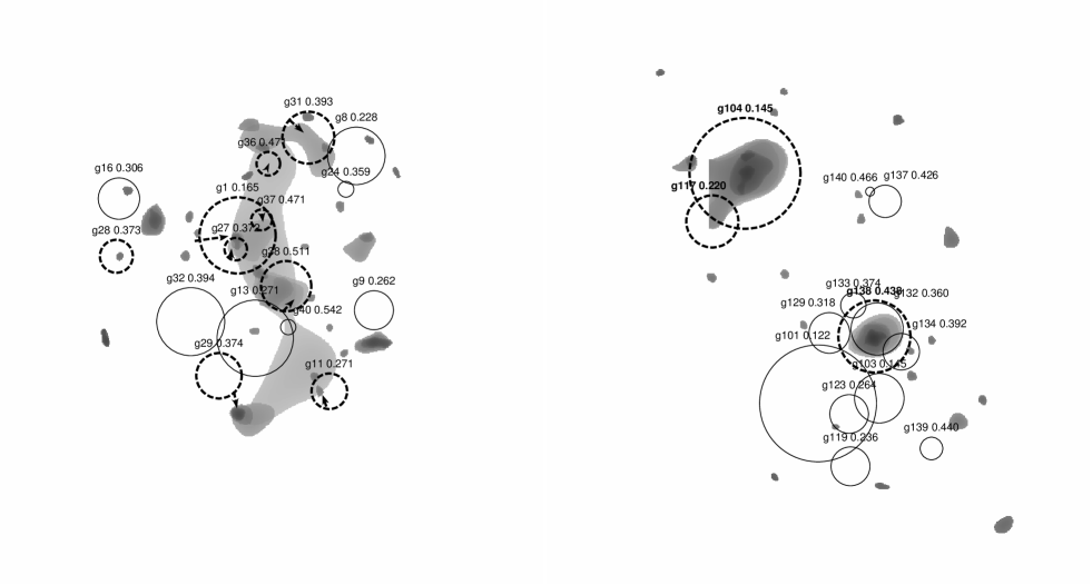
Figure 5.— Wavelet reconstruction of the X-ray surface brightness in the 0.5–2 keV band for the RA14h (left) and the RA21h (right) CNOC2 patches. Circles indicate the position and size ($R_{200}$) of the spectroscopically selected groups. Groups for which we were able to ascribe X-ray emission are shown as thick dashed circles. Groups without X-ray emission are shown as thin solid circles. In complex situations, arrows are used to make an assignment clear. Numerics refer to the spectroscopically selected group ID (from Carlberg et al. 2001) and corresponding redshift. Some of the assignment of X-ray emission to an optical group is tentative and is therefore not listed in Tab.1.

Fig.5 shows our best attempt to assign X-ray emission to the spectroscopically selected groups in the CNOC2 catalog (ids from Carlberg et al, 2001). In this case, the spectroscopic identification of the X-ray group was relaxed so that only two galaxies of matching redshift are required inside the area of X-ray emission. Circles at the position of spectroscopically selected groups indicate the area enclosed by $R_{200}$ (as computed by Balogh et al, 2007). Overlapping X-ray sources (confusion) are common within areas of this size, particularly in the deeper RA14h field. This can lead to confused association of groups and X-ray sources, as the distances between groups of all types can be as low or lower than uncertainties on their centroids. X-ray centers are good to 10-30″ while the luminosity weighted centers of spectroscopically selected groups rely strongly on membership allocation and especially redshift completeness, and while a median off-centering value is $\sim$15″  a factor of 3 larger deviations are also predicted (Wilman et al., 2009). This is less of a problem in the shallower RA21h field within which only highly significant and well separated groups are matched (20% of spectroscopic groups in the X-ray survey area). In contrast, the deep RA14h field has a substantially higher fraction of probable matches (56% of spectroscopic groups in the X-ray survey area), but confusion of sources and centering uncertainty sometimes lead to ambiguous assignation of groups. The largest offset seems to be an edge effect – only part of the rich galaxy group g29 entered the CNOC2 spectroscopic survey area. Allocated sources are indicated in Fig.5, and include probable identifications of confused X-ray sources. However we do not exclude the possibility that some associations are missed due to confused X-ray emission or as yet unidentified (in redshift) X-ray peaks.

We now discuss all cases of tentative assignment in the RA14h field individually. Two spectroscopically selected groups (ids g36, g37 at z=0.471) in the RA14h field are found in an area of very faint and extended X-ray emission. Detailed analysis shows a low surface brightness 4′ scale X-ray detection which corresponds to a highly extended and elongated collection of galaxies at $z=0.471$ linking the two groups. X-ray emission from each of these groups is too faint for individual detection, but corresponds to approximately $M_{200}\sim 2\times 10^{13}M_{\odot}$, assuming an equality of their contribution to the detected flux. Emission strictly associated with group g31 is marginal (1 $\sigma$ significance) and corresponds to a group mass of $1.4\pm 0.7\times 10^{13}M_{\odot}$ ($M_{200}$). Emission from the group g38 at $z=0.511$ is confused with the foreground group at $z=0.04$ (see §5). The X-ray emission present on 1′ scales (see Fig.5) can only be explained by a 0.04 group, with $M_{200}=7.3\pm 0.6\times 10^{12}M_{\odot}$. However, enhanced X-ray emission centered on g38 and a high density of galaxies at $z\sim 0.511$ coincident with this emission suggests that g38 can still contribute on smaller scales with an upper limit on mass of $M_{200}<6\times 10^{13}M_{\odot}$. The group g27 is cospatial with the group g01, but there is a small-scale elongation of X-ray emission coincident with the location of the core of g27 group. A corresponding mass estimate for g27 associated with this emission yields $M_{200}=2.4\pm 0.5\times 10^{13}M_{\odot}$. Of the groups g27, g31, g36, g37 and g38 none meets the criteria for inclusion into a table of X-ray groups. However all are likely emitters, and they are located in the zones with detected X-ray flux. Excluding these groups would lead to a lower limit of 25% (4/16) X-ray detections for spectroscopically selected groups in the RA14h field.

Predicted number density as a function of redshift, dN/dz/d$\Omega$ (dN/dz per unit area in deg²) of galaxy groups. The solid curve shows the prediction for systems found in the X-ray survey. Short (long) dashed line shows the prediction for $10^{13}M_{\odot}$ ($3\times 10^{13}M_{\odot}$) halos in WMAP5 cosmology. Gray histograms show the observed abundance of spectroscopically selected groups found in CNOC2 (solid) and DEEP2 (dashed) surveys.

Fig.6 presents a model of the redshift distribution of X-ray selected systems (solid line), adding the area and sensitivity of the two CNOC2 patches. This assumes a WMAP5 cosmology (Komatsu et al. 2008) and the $L_{X}-M$ relation from Rykoff et al. (2008) with evolutionary corrections discussed above. The short (long) dashed line illustrates the number density of halos of mass $\geq 10^{13}M_{\odot}$ ($3\times 10^{13}M_{\odot}$), and demonstrates the relative contribution of halos above these mass thresholds. The X-ray detection mass threshold (where the solid and dashed lines cross) increases with redshift, from below $10^{13}M_{\odot}$ at $z\lesssim 0.3$ to above $3\times 10^{13}M_{\odot}$ at $z\gtrsim 0.8$. X-ray selection at this depth provides groups at $0\lesssim z\lesssim 1$, and so although the total number of systems per square degree is high ($\sim$100), the expected match to spectroscopically selected groups within a more limited redshift interval is moderate. Nonetheless, the depth of our observations provides a peak in the redshift distribution at $0.2\lesssim z\lesssim 0.7$, which is well suited to the CNOC2 redshift range of $0.1\lesssim z\lesssim 0.55$. The solid gray histogram, illustrating the averaged number density of CNOC2 spectroscopically selected groups, contains roughly twice the number of X-ray groups within this redshift range. Thus, a naive estimate of X-ray detected groups would be $\sim 50\%$; however, we note that there is a strong variation in the efficiency of group detection in the CNOC2 survey that is not included here. Nonetheless, this effectively demonstrates that our X-ray survey provides a selection of groups down to a canonical mass value of $10^{13}M_{\odot}$, below which the use of X-ray selection is not yet established.

This contrasts with the situation at higher redshift, for which the number density of X-ray detected groups is expected to drop off as the detection threshold gets pushed to higher and higher mass. This is the case for the DEEP2 spectroscopically selected group sample (I) at $0.75<z<1.03$ from Gerke et al. (2007, dashed gray histogram), which shows that at exposures similar to our survey the full strength of the X-ray selection of galaxy groups is not yet exploited, while the DEEP2 spectroscopic galaxy group survey would allow a comparison down to the $10^{13}M_{\odot}$ mass limit.

The modeling in Fig.6 makes a simplistic assumption that the spectroscopic survey for galaxy groups is complete, which may introduce further differences between spectroscopic and X-ray selected group samples, which we consider next.

Probability of group detection as a function of halo mass at $z\sim 0.4$. Both X-ray selection at the depth of the RA14h field (dashed black curve) and spectroscopic selection in CNOC2 (including the effects of incompleteness, solid black curve) are modeled as described in the text. We ignored a possible covariance between optical richness and X-ray luminosity in predicting the percentage of groups only detected in X-rays (dashed gray line), the percentage of groups only detected spectroscopically (solid gray line) and the percentage of groups detected jointly (dotted gray line).

Fig.7 illustrates the recovery of groups as a function of halo mass, detected using both X-ray (at RA14h depth) and spectroscopic selection methods. The figure is constructed to show the percentage of groups detected as a function of mass, evaluated at a typical CNOC2 redshift $z=0.4$. X-ray groups are modeled as in Fig.6, and scatter in the Lx-M relation is ignored, providing a mass threshold which is a simple function of halo mass: the non-abrupt mass cut-off is merely a result of the variable depth across the RA14h field. Introducing scatter would introduce a higher sensitivity toward low-mass systems, smearing the boundary by additional 30% in mass (Vikhlinin et al. 2009). The modeling of the group recovery rate in the CNOC2 spectroscopic survey is based on applying the spectroscopic survey characteristics (including mean sampling rate) to the semi-analytic galaxy formation model in Millennium Simulation (Font et al. 2008), as described by McGee et al. (2008). Spectroscopically selected samples will inevitably include a large number of lower mass groups, as the drop in recovery rate is compensated by an increase in number density. The correlation of the richness and X-ray luminosity is accounted in the plot, while we ignored the second-order effects associated with the possible covariance in the deviation from the richness-mass and Lx-mass relations.

It is interesting to examine the expected mass of groups detected only by X-ray or spectroscopic methods, and the intersection between the two samples (indicated by gray lines in Fig.7) to complement the actual data. In the RA14h field, all three of the confirmed $0.14\leq z\leq 0.5$ X-ray selected groups are also in the spectroscopically selected sample (which is only sensitive to this limited redshift range). In the shallower RA21h field only three out of the ten $0.14\leq z\leq 0.5$ significant X-ray groups within the area covered by the CNOC2 survey are in the spectroscopically selected sample. Of the seven undetected groups, five have estimated masses less than $\sim 3\times 10^{13}M_{\odot}$; from Fig.7 we see that the spectroscopic completeness in this mass range is less than $\lesssim 80$ per cent, due primarily to the sparse sampling; therefore perfect recovery of such low-mass X-ray groups is not expected. However, two X-ray groups with masses $>7\times 10^{13}M_{\odot}$ are absent from the spectroscopic catalog. This may be due to the spatial variation of the spectroscopic completeness, which is not included in the completeness function of Fig. 7; we also note that group X21h13 is right near the edge of the CNOC2 coverage. Thus, overall we find 6/13 X–ray detected groups are also identified in an independent spectroscopic survey, over the area and redshift range that they can be fairly compared. This is approximately consistent with expectations, given the sparse sampling of that survey. Only one group is a surprising non-detection, given its estimated mass. Better sampled spectroscopy and improved mass estimates for these systems will help to understand this anomaly. But we find no convincing evidence for a substantial population of X–ray bright groups with no optical counterpart.

$L_{X}-\sigma$ relation for groups. The open points are our measurements of the flux attributed to the uniquely identified groups. The filled points correspond to detections of emission at the position of optical groups, but which are likely contaminated with emission from other groups. The $2\sigma$ upper limits are shown using short-dashed line ending with an arrow. 68% error bars are shown for the velocity dispersion measurements. In calculating the X-ray luminosity, the K-correction has been done iteratively using both the redshift of the source and the expected temperature given the evolved L–T relation (see Finoguenov et al. 2007 for details). The fits to the local sample data of Mulchaey et al. (2003), as presented in Spiegel et al., are shown as solid (inverse regression) and dashed (direct regression) lines. The fit to the $z\sim 0.25$ data of Rykoff et al. (2008) is shown as the dotted line. All fits were corrected for differences in the definition of energy band for calculating $L_{X}$ and evolution. We find no evidence for differences in the $L_{X}-\sigma$ relation for low and high redshift groups.

We now address the flip-side of this issue, on the X–ray detection of groups selected from optical spectroscopy. There has been recent discussion in the literature on the lack of detection of X-ray emission from optical groups at high redshifts (Spiegel et al. 2007; Fang et al. 2007). In particular, Spiegel et al. (2007) claim that their upper limits on the X-ray emission from the groups in the CNOC2 RA14h patch are mildly inconsistent with the optical-X-ray scaling relations found for the low redshift groups in Mulchaey et al. (2003). By combining X-ray data from Chandra and XMM-Newton, we are able to detect several groups which were not detected by Spiegel et al. (2007); furthermore, from our follow-up spectroscopy we have better determined velocity dispersion measurements (Wilman et al. 2005a). Based on these new measurements, we present in Fig.8 the X–ray luminosities and limits as a function of group velocity dispersion (the equivalent of Spiegel et al.’s Fig.4), for both the RA14h and RA21h patches. The evolved local relation is shown as the solid and dashed lines; these are based on the data of Mulchaey et al. (2003), as fit by Spiegel et al.; the two fits correspond to using either direct or inverse regression. We also show the best-fit relation of the $z\sim 0.25$ sample from Rykoff et al. (2008). All of our detections lie near or above these best-fit relations, and within the scatter defined by the Mulchaey et al. (2003) data. Moreover, all but two of our upper limits are consistent with these relations and, again, fully consistent within the scatter of those local data. Therefore we find no evidence for a significant difference between the X-ray properties of moderate redshift groups and local samples.

Moreover, we would like to outline a number of caveats that must be considered when comparing the CNOC2 groups with local samples. First, Mulchaey et al. (2003) was based on an archival ROSAT sample. Such archival samples tend to be dominated by X-ray bright systems (see discussion in Mulchaey 2000), which introduces a bias against high velocity dispersion, low $L_{X}$ groups. Therefore, a comparison between the optically-selected CNOC2 groups and the low redshift sample in Mulchaey et al. (2003) is not straightforward. In addition, the scatter in the $L_{X}-\sigma$ relation is large and requires as large a scatter in the $\sigma-M$ relation as in the $L_{X}-M$ relation, as confirmed in the analysis of numerical simulations (Biviano et al. 2006). Such an intrinsic scatter reduces the significance of deviations from the best-fit relation of any subsample, which was not taken into account in Spiegel et al. (2007). Thus, we find no evidence that high redshift groups are anomalously faint, as they would be if the gas had been subject to very strong preheating or feedback (e.g., Balogh et al. 2006). No significant evidence for systematic differences in X-ray properties between nearby and moderate-z groups is consistent with the results for the X-ray selected samples discussed by Jeltema et al. (2006).

8. Summary

We have presented an X-ray survey of two CNOC2 fields with Chandra and XMM-Newton and our method to find extended X-ray emission. We described preliminary results from the spectroscopic follow-up of the X-ray selected groups and provide a catalog of X-ray group candidates. To match spectroscopically and X-ray selected groups it is crucial to provide a full 3D match in redshift space. Centering issues mean a purely 2D match will always be insufficient, especially given incompleteness of spectroscopic surveys and the fact that current X-ray observations are only able to detect the central regions of groups. A probable detection of $\sim 50\%$ ($20\%$) of spectroscopically selected groups in the deeper (shallower) RA14h (RA21h) field demonstrates that a depth of $\geq$300 ksec with Chandra is crucial to reach the sensitivity necessary for X-ray detection of galaxy groups in the redshift range $0.1\lesssim z\lesssim 0.6$. The X-ray groups with identified spectroscopic redshifts have an ensemble-averaged weak lensing velocity dispersion of 309$\pm 106$ km s^-1. Finally we show that our current data show no statistically significant evidence for any mismatch between the X-ray and spectroscopically selected groups. However improved statistics and mass estimates, which we will have once on-going XMM, spectroscopic and multiwavelength datasets are complete and evaluated, will facilitate better comparison of X-ray and optical properties of groups and allow us to test the origin of scatter and evolution in the $L_{X}-M$ relation.

References

- (1) Appenzeller, I. et al. 1998, The Messenger 94, 1
- Balogh et al. (2006) Balogh, M. L., Babul, A., Voit, G. M., McCarthy, I. G., Jones, L. R., Lewis, G. F., & Ebeling, H. 2006, MNRAS, 366, 624
- Balogh et al. (2007) Balogh, M.L. et al. 2007, MNRAS, 374, 1169
- Biviano et al. (2006) Biviano, A., Murante, G., Borgani, S., Diaferio, A., Dolag, K., & Girardi, M. 2006, A&A, 456, 23
- Brainerd et al. (1996) Brainerd, T., Blandford, R., & Smail, I. 1996, ApJ, 466, 623
- Brunner et al. (2008) Brunner, H., Cappelluti, N., Hasinger, G., Barcons, X., Fabian, A. C., Mainieri, V., & Szokoly, G. 2008, A&A, 479, 283
- Carlberg et al. (2001) Carlberg, R.G. et al. 2001, ApJ, 552, 427
- (8) Clowe, D., Bradač, M., Gonzalez, A. H., Markevitch, M., Randall, S. W., Jones, C., and Zaritsky, D. 2006, ApJ, 648, L109
- (9) Eke, V. R. et al. 2005, MNRAS, 362, 1233
- Fahlman et al. (1994) Fahlman, G., Kaiser, N., Squires, G., & Woods, D. 1994, ApJ, 437, 56 Fahlman, G., Kaiser, N., Squires, G., and Woods, D., 1994, 437, 56
- Fang et al. (2007) Fang, T., Gerke, B., David, D., Newman, J., David, M., Nandra, K., Laird, E., Koo, D., Coil, A., Cooper, M., Croton, D., Yan, R., ApJ, 660, 27
- Fernández-Soto et al. (1999) Fernández-Soto, A., Lanzetta, K. M., & Yahil, A. 1999, ApJ, 513, 34
- Ferrando et al. (2003) Ferrando, P., et al. 2003, Proc. SPIE, 4851, 232
- (14) Finoguenov, A. et al. 2007, ApJS, 172, 182
- Font et al. (2008) Font, A. S., et al. 2008, MNRAS, 389, 1619
- (16) Geller, M. J., & Huchra, J. P. 1983, ApJS, 52, 61
- (17) Gerke, B. F. et al. 2005, ApJ, 625, 6
- Gerke et al. (2007) Gerke, B. F., et al. 2007, MNRAS, 376, 1425
- (19) Ghizzardi S., Molendi S. 2002, ESA SP-488
- Hoekstra et al. (1998) Hoekstra, H., Franx, M., Kuijken, K., & Squires, G. 1998, ApJ, 504, 636
- (21) Hoekstra, H., Franx, M., & Kuijken, K. 2000, ApJ, 532, 88
- (22) Hoekstra, H., Franx, M., Kuijken, K., Carlberg, R., Yee, H., Lin, H., Morris, S., Hall, P., Patton, D., Sawicki, M., and Wirth, G. 2001, ApJ, 548, L5
- Hoekstra et al. (2005) Hoekstra, H. and Hsieh, B. C. and Yee, H. K. C. and Lin, H., &Gladders, M. D. 2005, ApJ, 635, 73
- Hudson et al. (1998) Hudson, M. J., Gwyn, S. D. J., Dahle, H., & Kaiser, N. 1998, ApJ, 503, 531
- (25) Jeltema, T. E. et al. 2006, ApJ, 649, 649
- (26) Jeltema, T. E. et al. 2007, ApJ, 658, 865
- (27) Kawata, D. & Mulchaey, J. S. 2008, ApJ, 672, 53
- Kelson (2003) Kelson, D. D. 2003, PASP, 115, 688
- (29) Kirsch, M. G. F., et al. 2004, Proc. SPIE, 5488, 103
- Komatsu et al. (2009) Komatsu, E., et al. 2009, ApJS, 180, 330
- (31) Kubo, J. M., Stebbins, A., Annis, J., Dell’Antonio, I. P., Lin, H., Khiabanian, H., and Frieman, J. A. 2007, ApJ, 671, 1466
- (32) Leauthaud, A., et al. 2009, ApJ, subm.
- Luppino & Kaiser (1997) Luppino, G. A., & Kaiser, N. 1997, ApJ, 475, 20
- Mandelbaum et al. (2006) Mandelbaum, R., Seljak, U., Kauffmann, G., Hirata, C. M., & Brinkmann, J. 2006a, MNRAS, 368, 715
- (35) Mandelbaum, R., Seljak, U., Cool, R. J., Blanton, M., Hirata, C. M., and Brinkmann, J. 2006b, ApJ, 372, 758
- (36) McCarthy, I. G. et al. 2008, MNRAS, 383, 593
- (37) McGee, S. L. et al. 2008, MNRAS, 387, 1605
- Mulchaey (2000) Mulchaey, J. S. 2000, ARA&A, 38, 289
- (39) Mulchaey et al. 2003, ApJ Suppl., 145, 39
- (40) Mulchaey et al. 2006, ApJ, 646, 133
- (41) Parker, L. C., Hudson, M. J., Carlberg, R. G., and Hoekstra, H. 2005, ApJ, 634, 806
- Parker et al.. (2007) Parker, L. C. and Hoekstra, H. and Hudson, M. J. and van Waerbeke, L. and Mellier, Y. 2007, ApJ, 669, 21
- Rasmussen et al. (2006) Rasmussen, J., Ponman, T. J., Mulchaey, J. S., Miles, T. A., & Raychaudhury, S. 2006, MNRAS, 373, 653
- Rykoff et al. (2008) Rykoff, E. S., et al. 2008, MNRAS, 387, L28
- (45) Saxton, R. D., et al. 2005, 5 years of Science with XMM-Newton, 149
- Snowden et al. (2008) Snowden, S. L., Mushotzky, R. F., Kuntz, K. D., & Davis, D. S. 2008, A&A, 478, 615
- Spiegel et al. (2007) Spiegel, D. S., Paerels, F., & Scharf, C. A. 2007, ApJ, 658, 288
- (48) Vikhlinin, A., McNamara, B.R., Forman, W., et al. 1998, ApJ, 502, 558
- Vikhlinin et al. (2009) Vikhlinin, A., et al. 2009, ApJ, 692, 1033
- Watson et al. (2001) Watson, M. G., et al. 2001, A&A, 365, L51
- (51) Willis, J. P. et al. 2005, MNRAS, 364, 751
- Wilman et al. (2005a) Wilman, D. J. et al. 2005a, MNRAS, 358, 71
- (53) Wilman, D. J. et al. 2005b, MNRAS, 358, 88
- (54) Wilman, D. J. et al. 2008, ApJ, 680, 1009
- (55) Wilman, D. J., Oemler, A., Mulchaey, J. S., McGee, S. L., Balogh, M. L., & Bower, R. G. 2009, ApJ, 692, 298
- (56) Yee, H. K. C. et al. 2000, ApJS, 129, 475
- (57) Zabludoff & Mulchaey 1998, ApJ, 496, 39
- (58) Zhang, Y.-Y., Finoguenov, A., Böhringer, H., et al. 2004, A&A, 413, 49