Reconstruction of Markovian Master Equation parameters through symplectic tomography.

Abstract

In open quantum systems, phenomenological master equations with unknown parameters are often introduced. Here we propose a time-independent procedure based on quantum tomography to reconstruct the potentially unknown parameters of a wide class of Markovian master equations. According to our scheme, the system under investigation is initially prepared in a Gaussian state. At an arbitrary time $t$, in order to retrieve the unknown coefficients one needs to measure only a finite number (ten at maximum) of points along three time-independent tomograms. Due to the limited amount of measurements required, we expect our proposal to be especially suitable for experimental implementations.

I Introduction

Tomographic maps Asorey et al. (2007) can be considered a very useful tool for reconstructing the physical state or some other properties of many physical systems, both in a classical (e.g. medical physics, archaeology, biology, geophysics) and in a quantum perspective (e.g. photonic states Smithey et al. (1993), photon number distributions Brida et al. (2006); Zambra et al. (2005); Genovese et al. (2006), longitudinal motion of neutron wave packets Badurek et al. (2006)).

The tomographic analysis is based on a probabilistic approach towards physical system investigation. In particular, its key ingredient is the Radon transform Radon (1917). Given the phase-space of the system, this invertible integral transform allows to retrieve the marginal probability densities of the system, i.e. the probability density along straight lines. However, while in the classical regime the state of the system can be fully described by means of a probability distribution on its phase space, this is no longer the case of quantum systems. Indeed, due to the Heisenberg uncertainty relation, it is not possible to write a probability distribution as a function of both momentum and position. In this case, the Wigner function Wigner (1932); Moyal (1949) can be employed as a quantum generalization of a classical probability distribution. This function is a map between phase-space functions and density matrices. Even if the Wigner function can take on negative values, by integrating out either the position or the momentum degrees of freedom, one obtains a bona fide probability distribution for the conjugated variables. From this point of view, the Wigner function corresponding to a quantum state can be regarded as a quasi-probability distribution and interpreted as a joint probability density in the phase space Man’ko and Marmo (1999).

In this paper we apply quantum symplectic tomography to the investigation of open quantum systems Petruccione and Breuer (2002); Benatti and Floreanini (2005) which, due to the coupling to an environment (bath), undergo a non-unitary dynamical evolution. A complete microscopic description of system-plus-bath dynamics is a complex many-body problem. Hence, as in general one aims at describing the dynamics of the system, only basic information about the bath is retained, according to the so-called open system approach. The state of the system is then expressed by means of a reduced density matrix, obtained from the total density matrix by tracing out the environmental degrees of freedom. The system dynamics is then governed by the so-called quantum master equation. The master equation approach can be seen as the generalization of the Schrödinger equation to the possibly incoherent evolution of a density matrix. In this case, the generator of the time evolution is the Liouville dissipative operator. The integration of a time-dependent Liouvillian being a highly involved task, e. g. see Hu et al. (1992); Halliwell and Yu (1996), it is highly preferrable to deal with a time-independent Liouvillian, i.e. to assume a Markovian dynamics. Several approximations allow a Markovian description, such as the weak coupling limit, the singular limit and the low density limit Petruccione and Breuer (2002); Benatti and Floreanini (2005); Spohn (1980).
Nevertheless, a proper derivation of the master equation still requires complete information about the bath. The lack of this knowledge leads to the derivation of phenomenological master equations with unknown coefficients. Indeed, recent investigations Lidar et al. (2001); Schaller and Brandes (2008); Benatti et al. (2009) provide a more accurate approximation than the weak coupling limit, due to a more refined coarse grained dynamics. Even in this case, the obtained master equation has unknown coefficients, as it depends phenomenologically on the system investigated.

In this paper, we will focus on a class of Markovian master equations with unknown coefficients modeling a one-dimensional damped harmonic oscillator. In particular, we choose Lindblad operators Lindblad (1976) linear in both momentum and position degrees of freedom, such that the dynamical evolution of the system preserves the Gaussian form of the states. Our goal is to show how, by means of a tomographic approach, it is possible to measure indirectly the unknown coefficients by using Gaussian wave packets as a probe.

This paper is organized as follows. In section II we introduce the class of master equations we want to investigate. In section III we derive the expressions for the coefficients of the master equation as a function of the first and second evolved momenta (cumulants) of a Gaussian state. In section IV we introduce the Wigner function and the Radon transform for an arbitrary Gaussian wave packet at a generic time $t$ . We show that in order to measure the cumulants of a Gaussian state, and then indirectly the unknown parameters of the master equation, we need only a finite number (eight or ten) of time-independent tomograms. In section V we summarize and discuss our results and outline some feasible applications. Finally, in appendix A, we propose an alternative procedure to obtain the cumulants of a Gaussian state by means of time-dependent tomograms. This approach however appears to be less convenient for practical implementations.

II Description of the system

We want to investigate a class of master equations describing a Gaussian-shape-preserving (GSP) evolution of a quantum state. In the Markovian approximation, the non-unitary time evolution of a quantum system is described by the following general master equation Lindblad (1976); Gorini et al. (1976):

$$\frac{d\hat{\rho}(t)}{dt}= L(\hat{\rho}(t))$$

$$= - \frac{i}{\hslash}\left[\hat{H},\hat{\rho}(t)\right]$$ (1)

$$+ \frac{1}{2\hslash}\sum_{j}\left(\left[\hat{V}_{j}\hat{\rho}(t),\hat{V}_{j}^{\dagger}\right]+\left[\hat{V}_{j}\hat{\rho}(t)\hat{V}_{j}^{\dagger}\right]\right),$$

where $\hat{\rho}(t)$ is the reduced density operator of the system. Eq. (1) is exactly solvable if the Lindblad operators $\hat{V}_{j}$ and the system Hamiltonian $\hat{H}$ are, respectively, at most first and second degree polynomials in position ($\hat{q}$) and momentum ($\hat{p}$) coordinates Sandulescu and Scutaru (1987); Isar et al. (1994).

For systems like a harmonic oscillator or a field mode in an environment of harmonic oscillators (i.e. collective modes or a squeezed bath), $\hat{H}$ can be chosen of the general quadratic form

$$\hat{H}=\hat{H}_{0}+\frac{\delta}{2}\left(\hat{q}\hat{p}+\hat{p}\hat{q}\right),\qquad\hat{H}_{0}=\frac{1}{2m}\hat{p}^{2}+\frac{m\omega^{2}}{2}\hat{q}^{2},$$ (2)

where $\delta$ is the strength of the bilinear term in $\hat{q}$ and $\hat{p}$, $m$ is oscillator mass, and $\omega$ its frequency. The operators $\hat{V}_{j}$, which model the environment, are linear polynomials in $\hat{q}$ and $\hat{p}$:

$$\hat{V}_{j}=a_{j}\hat{p}+b_{j}\hat{q},\quad j=1,2,$$ (3)

with $a_{j}$ and $b_{j}$ complex numbers. The sum goes from $1$ to $2$ as there exist only two c-linear independent operators $\hat{V}_{1}$, $\hat{V}_{2}$, in the linear space of first degree polynomials in $\hat{p}$ and $\hat{q}$. We can safely omit generic constant contributions in $\hat{V}_{j}$ as they do not influence the dyamics of the system.

Given this choice of operators, the Markovian master equation (II) can be rewritten as:

$$\frac{\mathrm{d}\hat{\rho}(t)}{\mathrm{d}t} = \!-\frac{i}{\hslash}\left[\hat{H}_{0},\hat{\rho}(t)\right]-\frac{i(\lambda+\delta)}{2\hslash}\left[\hat{q},\hat{\rho}(t)\hat{p}+\hat{p}\hat{\rho}(t)\right]$$ (4)

$$+\frac{i(\lambda-\delta)}{2\hslash}\left[\hat{p},\hat{\rho}(t)\hat{q}+\hat{q}\hat{\rho}(t)\right]$$

$$-\frac{D_{pp}}{\hslash^{2}}\left[\hat{q},[\hat{q},\hat{\rho}]\right]-\frac{D_{qq}}{\hslash^{2}}\left[\hat{p},[\hat{p},\hat{\rho}(t)]\right]$$

$$+\frac{D_{qp}}{\hslash^{2}}\left(\left[\hat{q},[\hat{p},\hat{\rho}(t)]\right]+\left[\hat{p},[\hat{q},\hat{\rho}(t)]\right]\right)$$

where $\lambda=-\mathrm{Im}\sum_{j=1,2}a_{j}^{*}b_{j}$ is the unknown friction constant and

$$D_{qq} = \frac{\hslash}{2}\sum_{j=1,2}|a_{j}|^{2},\quad D_{pp}=\frac{\hslash}{2}\sum_{j=1,2}|b_{j}|^{2},$$

$$D_{qp} = -\frac{\hslash}{2}\mathrm{Re}\sum_{j=1,2}a_{j}^{*}b_{j}$$ (5)

are the unknown diffusion coefficients, satisfying the following constraints which ensure the complete positivity of the time evolution Sandulescu and Scutaru (1987); Isar et al. (1994):

$$i)D_{qq}>0,\quad ii)D_{pp}>0,\quad iii)D_{qq}D_{pp}-D_{qp}^{2}\geqslant\lambda^{2}\hslash^{2}/4.$$ (6)

Markovian GSP Master equations of the form Eq. (4) are used in quantum optics and nuclear physics Savage and Walls (1985); Kennedy and Walls (1988); Yang and Yannouleas (1986), and in the limit of vanishing $\omega$ can be employed for a phenomenological description of quantum Brownian motion Caldeira and Leggett (1983); Barnett and Cresser (2005); Bellomo et al. (2007). Also, in the case of a high-temperature Ohmic environment the time-dependent master equation derived in Hu et al. (1992); Halliwell and Yu (1996) can be recast in this time-independent shape. It must be noted however that in the high-temperature limit the third constrain in (6) seems to be violated. Nevertheless, even if $D_{qq}=0$, $D_{qp}=0$ and $\lambda\neq 0$, $D_{pp}$ diverges only linearly with temperature. Therefore, we can recover the complete positivity by means of a suitable renormalization. This renormalization consists in adding a suitable subleading term $D_{qq}$ (e.g. $D_{qq}\propto T^{-1}$). Otherwise, we can consider an high frequency cut-off for the environment Hu et al. (1992); Halliwell and Yu (1996). In this way the master equation is not Markovian anymore. Anyway, since it involves only regular functions, it should give a completely positive dynamics (as the microscopic unitary group does).

III Gaussian states evolution

In this section we investigate the evolution of an initial Gaussian state according to Eq. (4). In particular we derive invertible expressions for the cumulants of the state at a time $t$ in terms of the parameters of the master equation. Due to the Gaussian shape preservation, the evolved state at time $t$ is completely determined by its first and second order momenta:

$$\langle\hat{q}\rangle_{t} = {\rm Tr}(\hat{\rho}(t)\hat{q}),$$

$$\langle\hat{p}\rangle_{t} = {\rm Tr}(\hat{\rho}(t)\hat{p}),$$

$$\Delta q_{t}^{2} = {\rm Tr}(\hat{\rho}(t)\hat{q}^{2})-\langle\hat{q}\rangle^{2}_{t},$$

$$\Delta p_{t}^{2} = {\rm Tr}(\hat{\rho}(t)\hat{p}^{2})-\langle\hat{p}\rangle^{2}_{t},$$

$$\sigma(q,p)_{t} = {\rm Tr}\left(\hat{\rho}(t)\frac{\hat{q}\hat{p}+\hat{p}\hat{q}}{2}\right)-\langle\hat{q}\rangle_{t}\langle\hat{p}\rangle_{t}.$$ (7)

Due to the linearity of the $\hat{V}_{j}$’s in phase-space, the time-evolution of the first and second order cumulants can be decoupled. We then obtain the following two sets of solvable equations Sandulescu and Scutaru (1987); Isar et al. (1994):

$$\left\{\begin{array}[]{rl}\frac{d}{dt}\langle\hat{q}\rangle_{t}&=-(\lambda-\delta)\langle\hat{q}\rangle_{t}+\frac{1}{m}\langle\hat{p}\rangle_{t}\\ \\ \frac{d}{dt}\langle\hat{p}\rangle_{t}&=-m\omega^{2}\langle\hat{q}\rangle_{t}-(\lambda+\delta)\langle\hat{p}\rangle_{t}\end{array}\right.$$ (8)

$$\left\{\begin{array}[]{rl}\frac{d}{dt}\Delta q_{t}^{2}&\displaystyle=-2(\lambda-\delta)\Delta q_{t}^{2}+\frac{2}{m}\sigma(q,q)_{t}+2D_{qq}\\ \\ \frac{d}{dt}\Delta p_{t}^{2}&\displaystyle=-2(\lambda+\delta)\Delta p_{t}^{2}-2m\omega^{2}\sigma(q,p)_{t}+2D_{pp}\\ \frac{d}{dt}\sigma(q,p)_{t}&\displaystyle=-m\omega^{2}\Delta q_{t}^{2}+\frac{1}{m}\Delta p_{t}^{2}-2\lambda\sigma(q,p)_{t}+2D_{qp}\end{array}\right.$$ (9)

The above equations allow to obtain the time-dependent momenta as a function of the Master equation coefficients $\lambda,D_{qq},D_{pp},D_{qp}$. We now show how to invert these relations in order to express the parameters $\lambda,D_{qq},D_{pp},D_{qp}$ as a function of the evolved cumulants at an arbitrary time. The solution of Eqs. (8) is given by Sandulescu and Scutaru (1987); Isar et al. (1994)

$$\begin{cases}\langle\hat{q}\rangle_{t}=&\displaystyle e^{-\lambda t}\Bigg{[}\langle\hat{q}\rangle_{0}\left(\cosh\eta t+\frac{\delta}{\eta}\sinh\eta t\right)\\ &\displaystyle\qquad+\langle\hat{p}\rangle_{0}\frac{1}{m\eta}\sinh\eta t\Bigg{]}\\ \langle\hat{p}\rangle_{t}=&\displaystyle e^{-\lambda t}\Bigg{[}-\langle\hat{q}\rangle_{0}\frac{m\omega^{2}}{\eta}\sinh\eta t\\ &\displaystyle\qquad+\langle\hat{p}\rangle_{0}\left(\cosh\eta t-\frac{\delta}{\eta}\sinh\eta t\right)\Bigg{]},\end{cases}$$ (10)

where $\eta^{2}=\delta^{2}-\omega^{2}$. If $\eta^{2}<0$ we can set $\eta=i\Omega$ and the previous equations hold again with trigonometric instead of hyperbolic functions. The coefficient $\lambda$ can then be obained by inverting Eqs. (10).
The elements of the diffusion matrix can be retrieved from the second set of equations (9), whose solutions can be expressed in a compact form as

$$X(t)=(Te^{Kt}T)X(0)+TK^{-1}(e^{Kt}-1)TD,$$ (11)

where

$$X(t) = \begin{pmatrix}\displaystyle m\omega\Delta q_{t}^{2}\\ \displaystyle\frac{\Delta p_{t}^{2}}{m\omega}\\ \displaystyle\sigma(q,p)_{t}\end{pmatrix},\qquad D=\begin{pmatrix}\displaystyle 2m\omega D_{qq}\\ \displaystyle\frac{2D_{pp}}{m\omega}\\ \displaystyle 2D_{qp}\\ \end{pmatrix},$$

$$T = \frac{1}{2\eta}\begin{pmatrix}\delta+\eta&\delta-\eta&2\omega\\ \delta-\eta&\delta+\eta&2\omega\\ -\omega&-\omega&-2\delta\qquad\end{pmatrix},$$

$$K = \begin{pmatrix}-2(\lambda-\eta)&0&0\\ 0&-2(\lambda+\eta)&0\\ 0&0&-2\lambda\qquad\end{pmatrix}.$$ (12)

¿From the invertibility of matrices $T$ ($T^{2}=1$) and $\tilde{K}=K^{-1}\left(e^{Kt}-1\right)$ (invertible for bounded $K$ also if some of its eigenvalues are 0), we can derive the expression of $D_{qq}$, $D_{pp}$ and $D_{qp}$ using Eq. (11):

$$D = T\tilde{K}^{-1}T\left(X(t)-(Te^{Kt}T)X(0)\right),$$

$$\tilde{K} = K^{-1}(e^{Kt}-1)$$ (14)

$$= \begin{pmatrix}\displaystyle\frac{1-e^{-2(\lambda-\eta)}}{2(\lambda-\eta)}&0&0\\ 0&\displaystyle\frac{1-e^{-2(\lambda+\eta)}}{2(\lambda+\eta)}&0\\ 0&0&\displaystyle\frac{1-e^{-2\lambda}}{2\lambda}\end{pmatrix}.\quad$$

We emphasize that the time $t$ at which we are considering the cumulants is completely arbitrary. For instance, the expression of the coefficients $D_{qq},D_{pp},D_{qp}$ in terms of the asymptotic second cumulants and the parameter $\lambda$ reads:

$$D_{qq} = (\lambda-\delta)\Delta q_{\infty}^{2}-\frac{1}{m}\sigma(q,p)_{\infty},$$

$$D_{pp} = (\lambda+\delta)\Delta p_{\infty}^{2}+m\omega^{2}\sigma(q,p)_{\infty},$$

$$D_{qp} = \frac{1}{2}\left(m\omega^{2}\Delta q_{\infty}^{2}-\frac{1}{m}\Delta p_{\infty}^{2}+2\lambda\sigma(q,p)_{\infty}\right).$$

IV Cumulants reconstruction through tomography

In this section we introduce a procedure based on symplectic tomography in order to measure the first and second cumulants of a Gaussian wave packet at an arbitrary time $t$. This will allow us to indirectly measure the parameters $\lambda,D_{qq},D_{pp},D_{qp}$, them being functions of the evolved cumulants at an arbitrary time (see previous section). The tomographic approach is very useful when dealing with a phenomenological master equation of the form of Eq. (4), as the dependence of the coefficients of the master equation from the physical parameters is in principle unknown.

IV.1 Symplectic tomography

Given a quantum state $\hat{\rho}(t)$ its Wigner function reads:

$$W(q,p,t)=\frac{1}{\pi\hslash}\int_{-\infty}^{+\infty}\mathrm{d}y\exp\left(\frac{i2py}{\hslash}\right)\hat{\rho}(q-y,q+y,t).\\$$ (16)

If the system dynamics is described by the master equation (4), and the initial state is Gaussian, the Wigner function preserves the Gaussian form of the state. Indeed, it can be expressed as a function of its first and second order momenta:

$$W(q,p,t)=\frac{1}{2\pi\sqrt{\Delta q_{t}^{2}\Delta p_{t}^{2}-\sigma(q,p)_{t}^{2}}}$$

$$\times\exp\Bigg{[}-\frac{\Delta q_{t}^{2}(p-\langle\hat{p}\rangle_{t})^{2}+\Delta p_{t}^{2}(q-\langle\hat{q}\rangle_{t})^{2}}{2[\Delta q_{t}^{2}\Delta p_{t}^{2}-\sigma(q,p)_{t}^{2}]}$$

$$\qquad\quad-\frac{2\sigma(q,p)_{t}(q-\langle\hat{q}\rangle_{t})(p-\langle\hat{p}\rangle_{t})}{2[\Delta q_{t}^{2}\Delta p_{t}^{2}-\sigma(q,p)_{t}^{2}]}\Bigg{]}\,.$$ (17)

Let us now consider the line in phase-space

$$X-\mu q-\nu p=0.$$ (18)

The tomographic map of a generic state along this line, i.e. its Radon transform, is given by:

$$\varpi(X,\mu,\nu) = \langle\delta\left(X-\mu q-\nu p\right)\rangle$$

$$= \int_{\mathbb{R}^{2}}W(q,p,t)\delta\left(X-\mu q-\nu p\right)\mathrm{d}q\mathrm{d}p.$$

¿From equation  (IV.1) it follows that for a Gaussian wave packet the Radon transform can be explicitly written as:

$$\varpi(X,\mu,\nu)=\frac{1}{\sqrt{2\pi}\sqrt{\Delta q_{t}^{2}\mu^{2}+\Delta p_{t}^{2}\nu^{2}+2\sigma(q,p)_{t}\mu\nu}}\\ \exp\left[-\frac{\left(X-\mu\langle\hat{q}\rangle_{t}-\nu\langle\hat{p}\rangle_{t}\right)^{2}}{2[\Delta q_{t}^{2}\mu^{2}+\Delta p_{t}^{2}\nu^{2}+2\sigma(q,p)_{t}\mu\nu]}\right]\,,$$ (20)

with the following constraint on the second cumulants:

$$\Delta q_{t}^{2}\mu^{2}+\Delta p_{t}^{2}\nu^{2}+2\sigma(q,p)_{t}\mu\nu>0.$$ (21)

This constrain is obeyed for each value of the parameters $\mu$ and $\nu$ iff $\Delta q_{t}^{2}\Delta p_{t}^{2}-\sigma(q,p)_{t}^{2}>0$. This inequality is always satisfied as a consequence of the Robertson-Schrödinger relation.

Eq. (IV.1) also implies a homogeneity condition on the tomographic map: $|c|\,\varpi(cX,c\mu,c\nu)=\varpi(X,\mu,\nu)$. This condition can be used in the choice of parameters $\mu,\nu$. In fact, if one uses polar coordinates $(r,\theta)$, i.e. $\mu=r\cos\theta$, $\nu=r\sin\theta$, the homogeneity condition can be used to eliminate the parameter $r$. From Eq. (18) it emerges that the coordinates of the phase space need to be properly rescaled in order to have the same dimensions. For instance, we can set $q\to\sqrt{\frac{m\omega}{\hslash}}q$ and $p\to\sqrt{\frac{1}{\hslash m\omega}}p$. In particular if $\omega=0$, i.e. for a free particle interacting with the environment, we can choose the same rescaling with a fictitious frequency defined by $\hslash\bar{\omega}=\Delta p_{0}^{2}/2m$, imposing $q\to\frac{\Delta p_{0}}{\sqrt{2}\hslash}q$ and $p\to\frac{1}{\sqrt{2}\Delta p_{0}}p$. In general, every rescaling assigning the same dimensions to $q$ and $p$ is suitable for our purpose.

IV.2 From tomograms to cumulants

Let us now consider the tomograms corresponding to two different directions in phase space, i.e. to two different couples of parameters $(\mu,\nu)$, e. g. $X=q$ and $X=p$. These lines in phase space are associated respectively to the position and momentum probability distribution functions:

$$\varpi(X,1,0) = \frac{1}{\Delta q_{t}\sqrt{2\pi}}\exp\left[-\frac{\left(X-\langle\hat{q}\rangle_{t}\right)^{2}}{2\Delta q_{t}^{2}}\right],$$ (22)

$$\varpi(X,0,1) = \frac{1}{\Delta p_{t}\sqrt{2\pi}}\exp\left[-\frac{\left(X-\langle\hat{p}\rangle_{t}\right)^{2}}{2\Delta p_{t}^{2}}\right].$$ (23)

¿From Eqs. (22)-(23) we see that the tomographic map depends only on a single parameter $X$. This reduces the dimensionality of the problem with respect to the Wigner function, that is a function of both $p$ and $q$. The lines individuated by the choices $(\mu,\nu)=(1,0)$ and $(\mu,\nu)=(0,1)$ correspond to tomograms depending on the time average and variance respectively of position and momentum. In order to determine the latter quantities we have to invert Eq. (22) and (23) for different values of $X$, i.e. for a given number of points to measure along a tomogram. Thus, our first goal is to determine the number of tomograms required to measure the cumulants of our Gaussian state.

To answer this question, we first focus on the direction $\mu=1$, $\nu=0$. In Fig. 1 we plot the Wigner function of our system at a generic time $t$ and some straight lines along the considered direction. In Fig. 2 we plot the GSP tomogram defined by Eq. (22). Inverting Eq. (22), we obtain:

$$\left(X-\langle\hat{q}\rangle_{t}\right)^{2}=2\Delta q_{t}^{2}\ln\frac{1}{\varpi(X,1,0)\Delta q_{t}\sqrt{2\pi}}\,.$$ (24)

Using the value of the tomogram $\varpi(0,1,0)$ we can get $\langle\hat{q}\rangle_{t}$ as a function of $\Delta q_{t}$:

$$\langle\hat{q}\rangle_{t}=\pm\Delta q_{t}\sqrt{2\ln\frac{1}{\varpi(0,1,0)\Delta q_{t}\sqrt{2\pi}}}\,.$$ (25)

If we know the sign of $\langle\hat{q}\rangle_{t}$ then we need only the value of the tomogram $\varpi(0,1,0)$ to get $\langle\hat{q}\rangle_{t}$, otherwise we need another point. Using Eq. (25), Eq. (22) becomes an equation for $\Delta q_{t}$ only, and it can be rewritten as

$$2\Delta q_{t}^{2} \ln\frac{1}{\varpi(X,1,0)\Delta q_{t}\sqrt{2\pi}}$$

$$=\left(X\mp\Delta q_{t}\sqrt{2\ln\frac{1}{\varpi(0,1,0)\Delta q_{t}\sqrt{2\pi}}}\right)^{2}.$$

This equation is trascendental, therefore we will solve it numerically. We can graphically note in Fig. 3 that for each $X$ and corresponding $\varpi(X,1,0)$ there may be two values of $\Delta q_{t}$ satisfying the previous equation. In order to identify one of the two solutions, it is enough to consider two points, $\left\{(X_{1},\varpi(X_{1},1,0))\right\}$ and $\left\{(X_{2},\varpi(X_{2},1,0))\right\}$, and to choose the common solution for the variance. This is made clear by Fig. 3, where the ratio between right and left side of Eq. (IV.2) for two different values of $X$ is plotted. The common solution (i.e. when both ratios are equal to 1) is labeled $\overline{\Delta q}_{t}$.

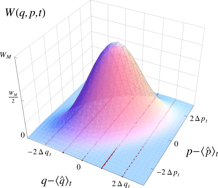
Figure 1: Wigner function, $W(q,p,t)$, of Eq. (IV.1) and some straight lines along the direction $\mu=1$ and $\nu=0$ on the plane $qp$. $\Delta q_{t}^{2}\Delta p_{t}^{2}-\sigma(q,p)_{t}^{2}=0.64\Delta q_{t}^{2}\Delta p_{t}^{2}$. $W_{M}=\frac{1}{2\pi\sqrt{\Delta q_{t}^{2}\Delta p_{t}^{2}-\sigma(q,p)_{t}^{2}}}$.

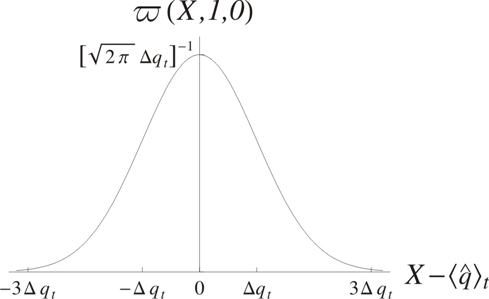
Figure 2: Tomogram, $\varpi(X,1,0)$, of Eq. (22) for the direction $\mu=1$ and $\nu=0$.

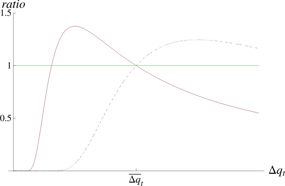
Figure 3: The ratio between right and left side of Eq. (IV.2) for two different values of $X$ with $\mu=1$ and $\nu=0$ is plotted as a function of $\Delta q_{t}$. Values used: $\langle\hat{q}\rangle_{t}=3$ and $X_{1}=4.5$ (continuous line) and $X_{2}=2.5$ (dashed line). The values of $\varpi(X,1,0)$ are computed using $\overline{\Delta q}_{t}=1$ to simulate what one would get experimentally. Continuous line shows how Eq. (IV.2) with $X_{1}=4.5$ and $\varpi(4.5,1,0)$ can be satisfied (ratio=1) by two values of $\Delta q_{t}$. The comparison with a second case with $X_{2}=2.5$ allows to determine which values of $\Delta q_{t}$ is the right one.

As a consequence, whether we know or not the sign of the average $\langle q\rangle_{t}$, we need three or four points to determine $\langle\hat{q}\rangle_{t}$ and $\Delta q_{t}$ in Eq. (22). Analogously, we need other three or four points for $\langle\hat{p}\rangle_{t}$ and $\Delta p_{t}$ in Eq. (23).

Let us now compute the covariance $\sigma(q,p)_{t}$. To this purpose, we consider the tomogram:

$$\varpi\left(X,\frac{1}{\sqrt{2}},\frac{1}{\sqrt{2}}\right)=\frac{1}{\sqrt{\pi}\sqrt{\Delta q_{t}^{2}+\Delta p_{t}^{2}+2\sigma(q,p)_{t}}}\\ \exp\left[-\frac{\left(X-\frac{\langle\hat{q}\rangle_{t}+\langle\hat{p}\rangle_{t}}{\sqrt{2}}\right)^{2}}{\Delta q_{t}^{2}+\Delta p_{t}^{2}+2\sigma(q,p)_{t}}\right].$$ (27)

This is a Gaussian whose average value is already determined. Indeed, according to the previous steps, we need two more points of this tomograms to determine the spread $(\Delta q_{t}^{2}+\Delta p_{t}^{2})/2+\sigma(q,p)_{t}$, from which we can retrieve $\sigma(q,p)_{t}$.

Hence, we have shown that by means of eight or at most ten points belonging to three tomograms, the first and second order momenta of a Gaussian state can be measured at an arbitrary time $t$. One can then use these measured cumulants in order to infer the master equation parameters describing the system under investigation. We note also that we can reasonably infer that the number of tomograms needed to reconstruct the system density operator is minimized by employing Gaussian wave packets as a probe. Indeed these states have minimum uncertainty, and are the only states having positive Wigner function Folland (1989).

V Conclusions

In this paper we have proposed an approach to the study of open quantum systems based on quantum symplectic tomography.

In many contexts the reduced dynamics of a system coupled with its environment is modeled by phenomenological master equations with some general features, but with unknown parameters. Hence, it would be highly appealing to find a way to assign some values to these parameters. We have tackled this problem for a wide class of Markovian master equations, which are the Gaussian-shape-preserving ones. We have proved that it is possible to retrieve their unknown parameters by performing a limited number (ten at maximum) of time-independent measurements using Gaussian wave packets as a probe.

This result leads to some interesting applications. Once retrieved the unknown master equation coefficients, it is possible to compute the dynamical evolution of any physical quantity whose analytical expression is known. The indirect-measurement scheme we propose could be then employed to make predictions on system loss of coherence due to the external environment. In order to perform this kind of analysis one can consider some quantities such as the spread and the coherence length in both position and momentum Franke-Arnold et al. (2001), provided their analytical expressions are available for an arbitrary time $t$ (e.g. see Ref.Bellomo et al. (2007)). Working in the coherent state representation, the evolution of the system of interest from an arbitrary initial state can be in principle predicted. Therefore, it is possible to perform the proposed indirect analysis of the decoherence processes. For example, if we consider an initial Schrödinger-cat state, highly interesting due to its potentially long-range coherence properties and its extreme sensitivity to environmental decoherence Brune et al. (1996), we can re-write it as a combination of four Gaussian functions. Therefore, due to the linearity of the master equation, it can be possible to derive analytically the state evolution and to analyze its loss of coherence by means of the procedure we propose.

VI Acknowledgements

We warmly thank Dr. P. Facchi, Prof. G. Marmo and Prof. S. Pascazio for many interesting and useful discussions. In particular we thank Prof. G. Marmo for his invitation at the University of Naples ”Federico II” which gave us the chance of starting this work.

Appendix A Alternative procedure

Here we propose an alternative time-dependent procedure to compute the second cumulants of a Gaussian state, by means of tomograms, given the knowledge of the first cumulants time evolution. To this purpose we need to consider the following three tomograms:

$$\varpi_{1} = \varpi(\langle\hat{p}\rangle_{t},0,1)=\frac{1}{\sqrt{2\pi}\Delta p_{t}}$$

$$\varpi_{2} = \varpi(\langle\hat{q}\rangle_{t},1,0)=\frac{1}{\sqrt{2\pi}\Delta q_{t}}$$

$$\varpi_{3} = \varpi\left(\frac{\langle\hat{p}\rangle_{t}+\langle\hat{q}\rangle_{t}}{\sqrt{2}},\frac{1}{\sqrt{2}},\frac{1}{\sqrt{2}}\right)$$ (28)

$$= \frac{1}{\sqrt{2\pi}\sqrt{\Delta q_{t}^{2}/2+\Delta p_{t}^{2}/2+\sigma(q,p)_{t}}}.$$

Inverting the previous equations one can infer $\Delta q_{t}$, $\Delta p_{t}$ and $\sigma(q,p)_{t}$ from the knowledge of $\varpi_{1}$, $\varpi_{2}$ and $\varpi_{3}$. However, this procedure presents two drawbacks. In fact, the evolved averaged values $\langle\hat{q}\rangle_{t}$ and $\langle\hat{p}\rangle_{t}$ are required and we need tomograms evaluated on time-dependent variables. These problems do not arise in the time-independent procedure, based only on tomograms for which no a priori knowledge on the Gaussian state is required. Nevertheless, in this alternative time-dependent scheme only three tomograms are required.

References

- Asorey et al. (2007) M. Asorey, P. Facchi, V. I. Man’ko, G. Marmo, S. Pascazio, and E. G. C. Sudarshan, Physical Review A 76, 012117 (2007).
- Smithey et al. (1993) D. T. Smithey, M. Beck, M. G. Raymer, and A. Faridani, Phys. Rev. Lett. 70, 1244 (1993).
- Brida et al. (2006) G. Brida, M. Genovese, F. Piacentini, and M. G. A. Paris, Optics Letters 31, 3508 (2006).
- Zambra et al. (2005) G. Zambra, A. Andreoni, M. Bondani, M. Gramegna, M. Genovese, G. Brida, A. Rossi, , and M. G. A. Paris, Phys. Rev. Lett. 95, 063602 (2005).
- Genovese et al. (2006) M. Genovese, G. Brida, M. Gramegna, M. Bondani, G. Zambra, A. Andreoni, A. Rossi, and M. Paris, Laser Physics 16, 385 (2006).
- Badurek et al. (2006) G. Badurek, P. Facchi, Y. Hasegawa, Z. Hradil, S. Pascazio, H. Rauch, J. Řeháček, and T. Yoneda, Physical Review A 73, 032110 (2006).
- Radon (1917) J. Radon, Mathematische-Physikalische Klasse 69, S. 262 (1917).
- Wigner (1932) E. P. Wigner, Quantum Semiclass. Opt. 40, 749 (1932).
- Moyal (1949) J. Moyal, Proc. Camb. Phil. Soc. 45, 99 (1949).
- Man’ko and Marmo (1999) V. I. Man’ko and G. Marmo, 1999 Phys. Scr. 60, 111 (1999).
- Petruccione and Breuer (2002) F. Petruccione and H. Breuer, The Theory of Open Quantum Systems (Oxford University, 2002).
- Benatti and Floreanini (2005) F. Benatti and R. Floreanini, Int. J. Mod. Phys. B 19, 3063 (2005).
- Hu et al. (1992) B. L. Hu, J. P. Paz, and Y. Zhang, Phys. Rev. D 45, 2843 (1992).
- Halliwell and Yu (1996) J. J. Halliwell and T. Yu, Phys. Rev. D 53, 2012 (1996).
- Spohn (1980) H. Spohn, Rev. Mod. Phys. 53, 569 (1980).
- Lidar et al. (2001) D. Lidar, Z. Bihary, and K. B. Whaley, Chem. Phys. 268, 35 (2001).
- Schaller and Brandes (2008) G. Schaller and T. Brandes, Phys. Rev. A 78, 022106 (2008).
- Benatti et al. (2009) F. Benatti, R. Floreanini, and U. Marzolino, Preprint (2009).
- Lindblad (1976) G. Lindblad, Commun. Math. Phys. 48, 119 (1976).
- Gorini et al. (1976) V. Gorini, A. Kossakowski, and E. C. G. Sudarshan, J. Math. Phys. 17, 821 (1976).
- Sandulescu and Scutaru (1987) A. Sandulescu and H. Scutaru, Annals of Physics 173, 211 (1987).
- Isar et al. (1994) A. Isar, A. Sandulescu, H. Scutaru, E. Stefanescu, and W. Scheid, Int. J. Mod. Phys. E 3, No. 2, 635 (1994).
- Savage and Walls (1985) C. M. Savage and D. F. Walls, Phys. Rev. A 32, 2316 (1985).
- Kennedy and Walls (1988) T. A. B. Kennedy and D. F. Walls, Phys. Rev. A 37, 152 (1988).
- Yang and Yannouleas (1986) S. Yang and C. Yannouleas, Nucl. Phys. A 460, 201 (1986).
- Caldeira and Leggett (1983) A. O. Caldeira and A. J. Leggett, Physica. A 121, 587 (1983).
- Barnett and Cresser (2005) S. M. Barnett and J.D. Cresser, Phys. Rev. A 72, 022107 (2005).
- Bellomo et al. (2007) B. Bellomo, S. Barnett, and J. Jeffers, Jour. Phys. A: Math. Theor. 40, 9437 (2007).
- Folland (1989) G. B. Folland, Harmonic analysis in phase space (Princeton University Press, 1989).
- Franke-Arnold et al. (2001) S. Franke-Arnold, G. Huyet, and S. M. Barnett, J. Phys. B 34, 945 (2001).
- Brune et al. (1996) M. Brune, E. Hagley, J. Dreyer, X. Maitre, A. Maali, C. Wunderlich, J. M. Raimond, and S. Haroche, Phys. Rev. Lett. 77, 4887 (1996).