Electrical conductivity of high-pressure liquid hydrogen by quantum Monte Carlo methods

Abstract

We compute the electrical conductivity for liquid hydrogen at high pressure using quantum Monte Carlo. The method uses Coupled Electron-Ion Monte Carlo to generate configurations of liquid hydrogen. For each configuration, correlated sampling of electrons is performed in order to calculate a set of lowest many-body eigenstates and current-current correlation functions of the system, which are summed over in the many-body Kubo formula to give AC electrical conductivity. The extrapolated DC conductivity at 3000 K for several densities shows a liquid semiconductor to liquid-metal transition at high pressure. Our results are in good agreement with shock-wave data.

Liquid hydrogen at high pressure has been the subject of intense experimental and theoretical research, because of its special place in the periodic table and its cosmic abundance. Understanding its behavior under high pressure and high temperature is important for revealing the properties of giant planets such as Jupiter and Saturn. Metallization of liquid hydrogen at high pressure is of particular interest. Experiments using shock waves have found a metallization transitionweir96 ; at a pressure of 140 GPa and temperature of 3000 K, liquid hydrogen has been reported to turn from an insulating fluid into a metallic one with a DC conductivity of about 2000 ($\Omega$ cm)^-1. However, theoretically, such a metallization process has not been very well understood. Mean-field density functional theory (DFT) calculations hohl97 and Quantum Molecular Dynamics (QMD) calculations collins01 ; redmer08 have been used to calculate the electrical conductivity in liquid hydrogen, but these methods neglect correlations between electrons. Such correlations are likely to be important for the accurate determination of transport properties. In this letter, we propose and apply an alternative ab-initio method which combines the Coupled Electron-Ion Monte Carlo (CEIMC) method pierleoni04 with the Correlation Function Quantum Monte Carlo (CFQMC) method ceperley88 ; hammond94 .

Within the CEIMC approach pierleoni04 ; delaney06 , the electrons and protons are simulated with separate but coupled Monte Carlo simulations, taking advantage of the separation of time scales in the Born-Oppenheimer approximation. The Born-Oppenheimer energy surface for the protons is determined using reptation quantum Monte Carlo (RQMC) baroni99 . After the proton system reaches equilibrium, we record uncorrelated samples of proton configurations, which are subsequently used to determine the electrical conductivity.

The many-body Kubo formula kubo57 for electrical conductivity is

$$\sigma_{\alpha\alpha}(\omega)= \frac{2\pi e^{2}(1-e^{-\beta\hbar\omega})}{m^{2}\omega\Omega Z}\sum_{k,n}|\langle k|\sum_{i}p_{\alpha}^{i}|n\rangle|^{2}\times$$ (1)

$$e^{-\beta E_{n}}\delta(E_{k}-E_{n}-\hbar\omega),$$

where $\alpha=x,y,z$; $e$ $(m)$ is electron charge (mass), $\Omega$ is the volume, $\beta$ is the inverse temperature, $\omega$ is the frequency, and $p_{\alpha}^{i}$ is the $\alpha$ component of the momentum operator for the $i$th electron. $|n\rangle$ and $E_{n}$ are many-body eigen-states and eigen-energies of the Hamiltonian, and $Z=\sum_{n}e^{-\beta E_{n}}$ the partition function.

The key challenge in evaluating the Kubo formula (Eq. 1) is to determine the sum over all many-body eigenstates of the system. We compute a number of the lowest-energy eigenstates, and the relevant matrix elements, using the CFQMC method ceperley88 , which we now explain. Consider the subspace spanned by a set of $M$ many-body basis states $f_{j}(\textbf{R})$, i.e., $\Phi_{i}(\textbf{R})=\sum_{j=1}^{M}d_{ij}f_{j}(\textbf{R}),$ where R represents electronic coordinates. The ground basis state, $f_{0}(\textbf{R})$, has Slater determinants of Kohn-Sham single electron orbitals times a Jastrow pair correlation and backflow correctionsdelaney06 ; pierleoni08 . For the excited basis states $f_{j}(\textbf{R}),j>0$, we use low-lying particle-hole excitations with respect to the ground state $f_{0}(\textbf{R})$.

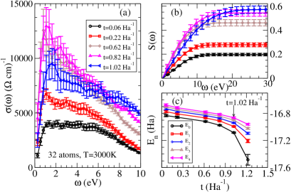
Figure 1: (Color online). Electrical conductivity (a), the corresponding sum rule (b), and five lowest energy levels (c) as a function of imaginary-time projection $t$ for $r_{s}=1.40$. Note the decrease of $\sigma(\omega)$ at low frequency is an artifact due to the gap in a finite system. The simulation has $M=24$ excited states. The results are averaged over 108 twist angles (see Fig. 3) and 10 decorrelated proton configurations drawn from the thermal Boltzmann distribution sampled by our CEIMC calculations. Lines are just guides to the eye.

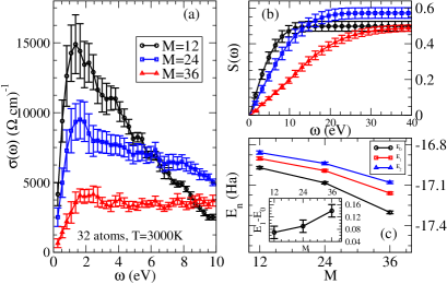
Figure 2: (Color online). Electrical conductivity (a), the corresponding sum rule (b), and first three lowest energy levels with energy difference $E_{1}-E_{0}$ in the inset as a function of $M$, the number of trial wavefunctions in the basis set. Here $t=1.02$ Ha^-1 for $r_{s}=1.40$.

Within this subspace, upper bounds to the exact eigenvalues can be found, by minimizing the Rayleigh quotient with respect to $d_{ij}$,

$$\Lambda_{i}=\frac{\int d\textbf{R}\Phi_{i}^{*}(\textbf{R})\hat{H}\Phi_{i}(\textbf{R})}{\int d\textbf{R}\Phi_{i}^{*}(\textbf{R})\Phi_{i}(\textbf{R})},$$ (2)

where $\hat{H}$ is the electronic Hamiltonian. Furthermore, an improved basis set $\{\tilde{f}_{i}(\textbf{R})\}$ can be obtained by applying an imaginary-time projection to the basis set:

$$\tilde{f}_{i}(\textbf{R})=e^{-t\hat{H}/2}f_{i}(\textbf{R}),$$ (3)

where $t$ is the projection time. Replacing $\{f_{j}(\textbf{R})\}$ with $\{\tilde{f}_{j}(\textbf{R})\}$ and minimizing $\Lambda_{i}$ with respect to $d_{ij}$, one obtains the many-body generalized eigenvalue equation:

$$\sum_{j=1}^{M}\textbf{H}_{ij}(t)d_{kj}(t)=\Lambda_{k}(t)\sum_{j=1}^{M}\textbf{S}_{ij}(t)d_{kj}(t),$$ (4)

where $\Lambda_{k}(t)$ is the $k$th eigenvalue, and the Hamiltonian H and the overlap matrices S are defined with respect to the projected basis set $\{\tilde{f}_{i}(\textbf{R})\}$ as

$$\textbf{H}_{ij} = \int d\textbf{R}_{1}d\textbf{R}_{2}f_{j}(\textbf{R}_{2})\langle\textbf{R}_{2}|\hat{H}e^{-t\hat{H}}|\textbf{R}_{1}\rangle f_{i}(\textbf{R}_{1}),$$ (5)

$$\textbf{S}_{ij} = \int d\textbf{R}_{1}d\textbf{R}_{2}f_{j}(\textbf{R}_{2})\langle\textbf{R}_{2}|e^{-t\hat{H}}|\textbf{R}_{1}\rangle f_{i}(\bf{R}_{1}).$$ (6)

Note that we have used Eq. (3) and inserted complete sets of basis states $\{|\textbf{R}\rangle\}$. These matrix elements are calculated all at once with RQMC.

Solving Eq. (4) yields the many-body eigenvalues and eigenfunctions that are required for the Kubo formula. The current-current correlation functions are computed at half of the projection time $t/2$ in RQMC ceperley88 . Finally, the $\delta$ function in the Kubo formula is broadened by a Gaussian function during the numerical calculation, whose width is of the same order as the observed many-body energy spacing.

We use the ground state as guiding wavefunction during RQMC simulations . The method is able to determine the lowest-lying states of the system, typically fewer than $50$ in our simulations, after which the calculation becomes less efficient due to the increased fluctuations in the matrix elements in Eqs. (5-6), a problem very much related to the well-known fermion sign problem of QMC. An analysis showsceperley88 that the Monte Carlo (MC) efficiency must decrease with projection time as $\exp(-\alpha t)$, making convergence in $t$ problematical: we call this the “efficiency problem”. However, it is important to note that as the basis is increased in size, the projected low energy states become more accurate ceperley88 . This suggests that we should include as many excitations as long as the efficiency is not severely reduced.

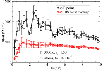
Figure 3: (Color online). Electrical conductivity calculated at the $\Gamma$ point compared with the twist-averaged one.

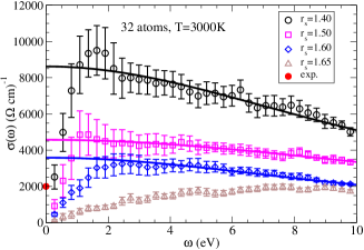
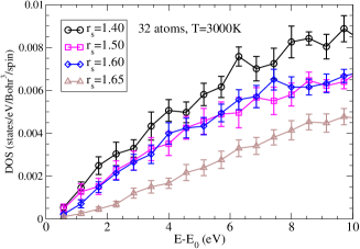
Figure 4: (Color online). Electrical conductivity (scattered points) along with the Drude fits (solid lines) (upper panel) and DOS (lower panel) as a function of density for liquid hydrogen. The red dot at $\omega=0$ indicates the experimental DC conductivity value after the liquid hydrogen is metallized by high pressure at 3000 K weir96 . The drop of electrical conductivity to zero at zero frequency for $r_{s}=1.40$, $1.50$ and $1.60$ is due to finite-size effects.

All simulations reported here were at 3000 K, the temperature of the shock experiments measuring conductivity weir96 . We first investigate the role of RQMC imaginary-time projection $t$. Fig. 1 (a) shows the electrical conductivity of liquid hydrogen as a function of $t$. Defining $S(\omega)=\frac{2m}{\pi en_{e}}\int_{0}^{\omega}\sigma(\omega^{{}^{\prime}})d\omega^{{}^{\prime}},$ the conductivity sum rule is $\lim_{\omega\rightarrow\infty}S(\omega)=1$ kubo57 . Here $n_{e}$ is electron density. In the present method, we cannot include all many-body states, so we do not expect the sum rule to be satisfied. However, it provides an indication of calculation quality. The main measure of appropriate projection time is the convergence of low-frequency $\sigma(\omega)$. We can see from Fig. 1 (a) that low-frequency $\sigma(\omega)$ curves converge between the interval $t\in[0.82,1.02]$Ha^-1. Here we choose the upper bound of $t=1.02{\rm Ha}^{-1}$, since we want to have as large $t$ as possible before the efficiency is reduced to an intolerable level. Note that the decrease in $\sigma(\omega)$ at $\omega<2$ eV is an artifact due to the finite number of atoms in the simulation, as we discuss below. Fig. 1 (b) also shows that the best sum rule satisfaction is achieved at $t=1.02{\rm Ha}^{-1}$, where $S(\omega)\sim 0.6$ as $\omega\rightarrow\infty$. As a further test of the $t$ value, we show in Fig. 1 (c) five lowest energy states as a function of projection time. We see that indeed after $t=1.02{\rm Ha}^{-1}$, the statistical variances increase substantially, and the estimates of the lowest energies are pushed down due to the noise hammond94 .

Fig. 2 shows (a) the electrical conductivity, (b) the corresponding $S(\omega)$, and (c) the first 3 energy levels at fixed projection time as a function of $M$, the size of the basis set. As before, we choose $M$ as large as possible while still obtaining a reasonable MC efficiency. To check the efficiency, we collect the same amounts of stochastic data for the Hamiltonian and overlap matrices in Eq. 5 and 6, solve the generalized eigenvalue equation Eq. 4, and look at the energy gap between ground state $E_{0}$ and the first excited state $E_{1}$. A sudden increase of the energy gap indicates the reduction of the efficiency, since noise can push down the most the lowest energy level hammond94 . The inset of Fig. 2 (c) shows an increased slope for $E_{1}-E_{0}$ curve at $M=36$, indicating such a reduction of efficiency. The corresponding $\sigma(\omega)$ curve is also suppressed in the low frequency region. See Fig. 2 (a). We find that $M=24$ is a good compromise between accuracy and efficiency. We also notice from Fig. 2 (b) that $S(\omega)\rightarrow 0.6$ as $\omega\rightarrow\infty$ for $M=24$; while for $M=12$ and $36$, the corresponding sum approaches $0.5$.

We note that our simulations are subject to finite-size errors in evaluating thermodynamic properties. Such effects can be reduced by using twist-averaged boundary conditions lin01 . In Fig. 3 we compare $\sigma(\omega)$ calculated at the $\Gamma$ point of the Brillouin zone (BZ) to the one averaged over a $6\times 6\times 6$ grid in the twist angle space (the BZ). We find that $\Gamma$ point sampling overestimates the conductivity value. However, finite-size effects have not been entirely eliminated and are responsible for the observed vanishing of $\sigma(\omega)$ at small $\omega$ for all systems studied. This will not happen for a sufficiently large system in the metallic phase (e.g. at $r_{s}\leq 1.50$). A common proceduregalli90 ; collins01 ; galli00 to estimate the DC conductivity is to discard a few data points and extrapolate the higher frequency data to $\omega=0$ . For systems inside the metallic phase one can use the Drude formula $\sigma(\omega)=\sigma_{\rm DC}/(1+\omega^{2}\tau^{2})$ to estimate the DC conductivity $\sigma_{\rm DC}$ and the electronic relaxation time $\tau$.

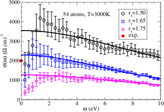
Figure 5: (Color online). Electrical conductivity (scattered points) and Drude fits (solid lines) as a function of density for liquid hydrogen. The red dot at $\omega=0$ denotes the experimental DC conductivity value after the liquid hydrogen is metallized by high pressure weir96 .

We now proceed to study the electrical conductivity at various densities at T= 3000 K, where the metallization of liquid hydrogen has been observed weir96 . We run CEIMC simulations at $r_{s}=1.40$, 1.50, 1.60, and 1.65 for 32 protons and electrons. Results (scattered points) along with the corresponding Drude fits (solid lines) are shown on the upper panel of Fig. 4 and many-body density of states (DOS) on the lower panel, where all the energy values are calculated with respect to the ground-state energy of the configuration. We can see that DC conductivity decreases from about 8600 $(\Omega$ cm$)^{-1}$ (see below) at $r_{s}=1.40$ to about $3500$ $(\Omega$ cm$)^{-1}$ at $r_{s}=1.60$ and to nearly zero at $r_{s}=1.65$. The dot at $\omega=0$ in Fig. 4 shows the experimental DC conductivity after metallization weir96 . The conductivity points for $r_{s}=1.65$ near zero frequency has typical features for liquid semiconductors, while a $2000$ $(\Omega$ cm$)^{-1}$ is a typical liquid metal value shimoji77 . Thus, based on 32-atom simulations we see a liquid metal to a liquid semiconductor transition in a density region of $1.60<r_{s}<1.65$ at T=3000 K for liquid hydrogen under high pressure, which is close to the experimental transition density of $r_{s}=1.62$. Such a metal-semiconductor transition is also hinted in the DOS figure. Going from $r_{s}=1.40$ to $r_{s}=1.65$, one can see the gradual opening of an energy gap.

We further look at the metallic behavior of the liquid hydrogen at $r_{s}=1.40$. The Drude fit gives $\sigma_{\rm DC}=8620\pm 1000$ $(\Omega$ cm$)^{-1}$ and $\tau=2.0\pm 0.2$ a.u. or $3.1\pm 0.3\times 10^{-16}$ s. A rough estimate of electron mean free path ($l$) then gives $l\sim 1.2$ Å, which is about 1.5 times the average proton-proton distance (1.4 Bohr) delaney06 , necessary for the system being metallic. For $r_{s}=1.50$ and 1.60 we also fit $\sigma(\omega)$ points to the Drude formula. The fitted curves become flatter as the density decreases, which signals that at $r_{s}=1.60$, liquid hydrogen has a small electronic relaxation time, making it a bad metal, similar to liquid carbon galli90 .

Finally, we explicitly test the importance of finite-size effects by performing simulations for 54-atom cells as shown in Fig. 5. The energy gap at $r_{s}=1.65$ that is present in the 32 atom simulation now disappears. The liquid semiconductor [at $r_{s}=1.75$ the extrapolated DC conductivity is around 1300 $(\Omega$ cm$)^{-1}$ less than a typical liquid metal value shimoji77 ; mott71 , hence the name] to liquid metal transition density is estimated to be in the range $1.65\leq r_{s}\leq 1.75$, which is again close to the experimental density of $r_{s}=1.62$ weir96 . Further increase of system size is not possible at present, but previous CEIMC calculations have found that the ground-state energy with 54 and 108 atoms are very close if twist-averaged boundary conditions are used. Therefore, we expect that the liquid metal transition density determined above is close to the thermodynamic limit. A more definitive answer will require significant additional calculations.

We have proposed a method to calculate the frequency dependent electrical conductivity using CEIMC with correlated Monte Carlo sampling and the many-body Kubo formula. The method is able to estimate some of the lowest-lying energies and their corresponding overlap matrices, and hence it is suitable for the extrapolation of DC conductivity from the AC conductivity. With this method we study the DC conductivity of liquid hydrogen as a function of density at 3000 K and at high pressure, and show the metallization. Our DC conductivity values at the metallization point is in good agreement with the shock-wave experiments weir96 . Furthermore, our metallization density ($r_{s}\sim 1.65$) is close to the experimental value of $r_{s}=1.62$. In the future, it will be interesting to apply the method to more densities and temperatures to have a complete understanding of liquid hydrogen electronic transport properties. It is also very promising to extend our method to other systems, such as lattice models.

F.L. thanks Michele Casula for helpful discussions. C.P. thanks the Institute of Condensed Matter Theory at the University of Illinois at Urbana-Champaign for a short term visit. This research was sponsored in part by the National Nuclear Security Administration under the Stewardship Science Academic Alliances program through DOE Grant DE-FG52-06NA26170; Ministero dell’Istruzione, dell’Universita e della Ricerca Grant PRIN2007 (to C.P.). Computer time was provided by NCSA at the University of Illinois at Urbana-Champaign and CINECA, Italy.

References

- (1) S. T. Weir, A. C. Mitchell, and W. J. Nellis, Phys. Rev. Lett. 76, 1860 (1996); W. J. Nellis, S. T. Weir, and A. C. Mitchell, Phys. Rev. B59, 3434 (1999).
- (2) O. Pfaffenzeller and D. Hohl, J. Phys.: Condens. Matter 9, 11023 (1997).
- (3) L. A. Collins et al., Phys. Rev. B63, 184110 (2001).
- (4) B. Holst, R. Redmer, and M. P. Desjarlais, Phys. Rev. B77, 184201 (2008).
- (5) C. Pierleoni, D. M. Ceperley, and M. Holzmann, Phys. Rev. Lett. 93, 146402 (2004); C. Pierleoni and D. M. Ceperley, Chem. Phys. Chem. 6, 1872 (2005); ibid, Lecture Notes in Physics 703, 641 (2006).
- (6) D. M. Ceperley and B. Bernu, J. Chem. Phys. 89, 6316 (1988); B. Bernu, D. M. Ceperley, and W. A. Lester Jr., J. Chem. Phys. 93, 552 (1990).
- (7) B. L. Hammond, W. A. Lester Jr., and P. J. Reynolds, Monte Carlo methods in ab initio quantum chemistry, Chap. 6, World Scientific, Singapore (1994).
- (8) K. T. Delaney, C. Pierleoni, and D. M. Ceperley, Phys. Rev. Lett. 97, 235702 (2006).
- (9) S. Baroni and S. Moroni, Phys. Rev. Lett. 82, 4745 (1999).
- (10) R. Kubo, J. Phys. Soc. Japan 12, 570 (1957).
- (11) C. Lin, F. H. Zong, and D. M. Ceperley, Phys. Rev. E64, 016702 (2001).
- (12) G. Galli, R. M. Martin, R. Car, and M. Parrinello, Phys. Rev. B42, 7470 (1990).
- (13) C. Pierleoni, K. T. Delaney, M. A. Morales, D. M. Ceperley, and M. Holzmann, Comp. Phys. Comm. 179, 89 (2008).
- (14) G. Galli, R. Q. Hood, A. U. Hazi, and F. Gygi, Phys. Rev. B61, 909 (2000).
- (15) M. Shimoji, Liquid Metals, p. 381, Academic Press, London (1977).
- (16) N. F. Mott, Philos. Mag. 24, 2 (1971).