Image Reconstruction in Optical Interferometry

Abstract

This tutorial paper describes the problem of image reconstruction from interferometric data with a particular focus on the specific problems encountered at optical (visible/IR) wavelengths. The challenging issues in image reconstruction from interferometric data are introduced in the general framework of inverse problem approach. This framework is then used to describe existing image reconstruction algorithms in radio interferometry and the new methods specifically developed for optical interferometry.

Index Terms – aperture synthesis, interferometry, image reconstruction, inverse problems, regularization.

I Introduction

Since the first multi-telescope optical interferometer [1], considerable technological improvements have been achieved. Optical (visible/IR) interferometers are now widely open to the astronomical community and provide means to obtain unique information from observed objects at very high angular resolution (sub-milliarcsecond). There are numerous astrophysical applications: stellar surfaces, environment of pre-main sequence or evolved stars, central regions of active galaxies, etc. See [2, 3, 4] for comprehensive reviews about optical interferometry and recent astrophysical results. As interferometers do not directly provide images, reconstruction methods are needed to fully exploit these instruments. This paper aims at reviewing image reconstruction algorithms in astronomical interferometry using a general framework to formally describe and compare the different methods.

Multi-telescope interferometers provide sparse measurements of the Fourier transform of the brightness distribution of the observed objects (cf. Section II). Hence the first problem in image reconstruction from interferometric data is to cope with voids in the sampled spatial frequencies. This can be tackled in the framework of inverse problem approach (cf. Section III). At optical wavelengths, additional problems arise due to the missing of part of Fourier phase information, and to the non-linearity of the direct model. These issues had led to the development of specific algorithms which can also be formally described in the same general framework (cf. Section IV).

II Interferometric Data

The instantaneous output of an optical interferometer is the so-called complex visibility $V_{j_{1},j_{2}}(t)$ of the fringes given by the interferences of the monochromatic light from the $j_{1}$-th and the $j_{2}$-th telescopes at instant $t$ [3]:

$$V_{j_{1},j_{2}}(t)=g_{j_{1}}(t)^{\star}\,g_{j_{2}}(t)\,\hat{I}\left(\boldsymbol{\nu}_{j_{1},j_{2}}(t)\right)$$ (1)

where $\hat{I}(\boldsymbol{\nu})$ is the Fourier transform of $I(\boldsymbol{\theta})$, the brightness distribution of the observed object in angular direction $\boldsymbol{\theta}$, $g_{j}(t)$ is the complex amplitude throughput for the light from the $j$-th telescope and $\boldsymbol{\nu}_{j_{1},j_{2}}(t)$ is the spatial frequency sampled by the pair of telescopes $(j_{1},j_{2})$ (see Fig. 1):

$$\boldsymbol{\nu}_{j_{1},j_{2}}(t)=\frac{\boldsymbol{r}_{j_{2}}(t)-\boldsymbol{r}_{j_{1}}(t)}{\lambda}$$ (2)

with $\lambda$ the wavelength and $\boldsymbol{r}_{j}(t)$ the projected position of the $j$-th telescope on a plane perpendicular to the line of sight. These equations assume that the diameters of the telescopes are much smaller than their projected separation and that the object is an incoherent light source. An interferometer therefore provides sparse measurements of the Fourier transform of the brightness distribution of the observed object. The top-left panel of Fig. 2 shows an example of the sampling of spatial frequencies by an interferometer.

In practice, the complex visibility is measured during a finite exposure duration:

$$V_{j_{1},j_{2},m}^{\mathsf{data}}=\langle V_{j_{1},j_{2}}(t)\rangle_{m}+V_{j_{1},j_{2},m}^{\mathsf{err}}$$ (3)

where $\langle\,\rangle_{m}$ denotes averaging during the $m$-th exposure and $V_{j_{1},j_{2},m}^{\mathsf{err}}$ stands for the errors due to noise and modeling approximations. The exposure duration is short enough to consider the projected baseline $\boldsymbol{r}_{j_{2}}(t)-\boldsymbol{r}_{j_{1}}(t)$ as constant, thus:

$$\langle V_{j_{1},j_{2}}(t)\rangle_{m}\simeq G_{j_{1},j_{2},m}\,\hat{I}\left(\boldsymbol{\nu}_{j_{1},j_{2},m}\right)$$ (4)

with $\boldsymbol{\nu}_{j_{1},j_{2},m}=\langle\boldsymbol{\nu}_{j_{1},j_{2}}(t)\rangle_{m}\simeq\boldsymbol{\nu}_{j_{1},j_{2}}(t_{m})$, $t_{m}=\langle t\rangle_{m}$ the mean exposure time and $G_{j_{1},j_{2},m}=\langle g_{j_{1}}(t)^{\star}\,g_{j_{2}}(t)\rangle_{m}$ the effective optical transfer function (OTF). The fast variations of the instantaneous OTF are mainly due to the random optical path differences (OPD) caused by the atmospheric turbulence. In long baseline interferometry, two telescopes are separated by more than the outer scale of the turbulence, hence their OPDs are independent. Furthermore, the exposure duration is much longer than the evolution time of the turbulence (a few $10\,$ms) and averaging can be approximated by expectation:

$$\langle g_{j_{1}}(t)^{\star}\,g_{j_{2}}(t)\rangle_{m}\simeq\mathrm{E}\left\{g_{j_{1}}(t)^{\star}\right\}_{m}\,\mathrm{E}\left\{g_{j_{2}}(t)\right\}_{m}$$

with $\mathrm{E}\{\}_{m}$ the expectation during the $m$-th exposure. During this exposure, the phase of $g_{j}(t)$ is $\phi_{j}(t)=\phi_{j,m}+(2\,\pi/\lambda)\,\delta_{j}(t)$ with $\phi_{j,m}=\langle\phi_{j}(t)\rangle_{m}$ the static phase aberration and $\delta_{j}(t)\sim\mathcal{N}(0,\sigma_{\delta}^{2})$ the OPD which is a zero-mean Gaussian variable with the same standard deviation for all telescopes [5]. For a given telescope, the amplitude and phase of the complex throughput can be assumed independent, hence:

$$\mathrm{E}\left\{g_{j}(t)\right\}_{m}\simeq\mathrm{E}\left\{|g_{j}(t)|\right\}_{m}\,\mathrm{E}\bigl{\{}\mathrm{e}^{\mathrm{i}\,\phi_{j}(t)}\bigr{\}}_{m}\simeq g_{j,m}\,\mathrm{e}^{-\frac{1}{2}\sigma_{\phi}^{2}}$$

with $g_{j,m}=|g_{j}(t_{m})|\,\exp(-\mathrm{i}\,\phi_{j,m})$ and $\sigma_{\phi}^{2}=(2\,\pi/\lambda)^{2}\,\sigma_{\delta}^{2}$ the variance of the phase during an exposure. The OTF is finally:

$$G_{j_{1},j_{2},m}=\langle g_{j_{1}}(t)^{\star}\,g_{j_{2}}(t)\rangle_{m}\simeq g_{j_{1},m}^{\star}\,g_{j_{2},m}\,\mathrm{e}^{-\sigma_{\phi}^{2}}\,.$$ (5)

At long wavelengths (radio), the phase variation during each exposure is small, hence $G_{j_{1},j_{2},m}\simeq g_{j_{1},m}^{\star}\,g_{j_{2},m}\not=0$. If some means to calibrate the $g_{j,m}$’s are available, then image reconstruction amounts to deconvolution (cf. Section III); otherwise, self-calibration (cf. Section III-H) has been developed to jointly estimate the OTF and the brightness distribution of the object given the measured complex visibilities.

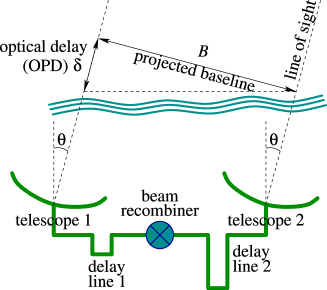
Figure 1: Geometrical layout of an interferometer. $B$ is the projected baseline, $\theta$ is the view angle and $\delta$ is the geometrical optical path difference which is compensated by the delay lines.

At short wavelengths (optical), the phase variance exceeds a few squared radians and $G_{j_{1},j_{2},m}\simeq 0$, hence the object’s complex visibility cannot be directly measured. A first solution would be to compensate for the OPD errors in real time using fast delay lines. This solution however requires a bright reference source in the vicinity of the observed object and dedicated instrumentation [6] that is currently in development and not yet available. An alternative solution consists in integrating non-linear estimators that are insensitive to telescope-wise phase errors. This requires high acquisition rates (about $1000\,\mathrm{Hz}$ in the near infrared) and involves special data processing but otherwise no special instrumentation.

To overcome loss in visibility transmission due to fast varying OPD errors, current optical interferometers integrate the power spectrum (for $j_{1}\not=j_{2}$):

$$S_{j_{1},j_{2},m}=\langle|V_{j_{1},j_{2}}(t)|^{2}\rangle_{m}\simeq\rho_{j_{1},m}\,\rho_{j_{2},m}\,|\hat{I}(\boldsymbol{\nu}_{j_{1},j_{2},m})|^{2}\,,$$ (6)

with $\rho_{j,m}=\langle|g_{j}(t)|^{2}\rangle_{m}$ the mean squared modulus of the complex throughput of the $j$-th telescope during the $m$-th exposure. By construction, the $\rho_{j,m}$’s are insensitive to the phase errors and so is the power spectrum. Unlike that of the complex visibility, the transfer function $\rho_{j_{1},m}\,\rho_{j_{2},m}$ of the power spectrum is not negligible. This transfer function can be estimated by simultaneous photometric calibration and, to compensate for remaining static effects, from the power spectrum of a reference source (a so-called calibrator). Hence the object power spectrum $|\hat{I}(\boldsymbol{\nu}_{j_{1},j_{2},m})|^{2}$ can be measured by $S_{j_{1},j_{2},m}$ in spite of phase errors due to the turbulence.

To obtain Fourier phase information (which is not provided by the power spectrum), the bispectrum of the complex visibilities is measured:

$$B_{j_{1},j_{2},j_{3},m} =\langle V_{j_{1},j_{2}}(t)\,V_{j_{2},j_{3}}(t)\,V_{j_{3},j_{1}}(t)\rangle_{m}$$

$$\simeq\rho_{j_{1},m}\,\rho_{j_{2},m}\,\rho_{j_{3},m}\,$$

$$\quad{}\times\hat{I}(\boldsymbol{\nu}_{j_{1},j_{2},m})\,\hat{I}(\boldsymbol{\nu}_{j_{2},j_{3},m})\,\hat{I}(\boldsymbol{\nu}_{j_{3},j_{1},m})\,,$$ (7)

where $j_{1}$, $j_{2}$ and $j_{3}$ denote three different telescopes. As for the power spectrum, the transfer function $\rho_{j_{1},m}\,\rho_{j_{2},m}\,\rho_{j_{3},m}$ of the bispectrum can be calibrated. Since this transfer function is real, it has no effect on the phase of the bispectrum (the so-called phase closure) which is equal to that of the object:

$$\beta_{j_{1},j_{2},j_{3},m} \equiv\arg(B_{j_{1},j_{2},j_{3},m})$$

$$=\arg(\hat{I}(\boldsymbol{\nu}_{j_{1},j_{2},m})\,\hat{I}(\boldsymbol{\nu}_{j_{2},j_{3},m})\,\hat{I}(\boldsymbol{\nu}_{j_{3},j_{1},m}))\,.$$ (8)

Some phase information is however missing. Indeed, from all the interferences between $T$ telescopes (in a non-redundant configuration), $T\,(T-1)/2$ different spatial frequencies are sampled but the phase closure only yields $(T-1)\,(T-2)/2$ linearly independent phase estimates [3]. The deficiency of phase information is most critical for a small number of telescopes. Whatever the number of telescopes is, at least the information of absolute position of the observed object is lost.

In practice, obtaining the power spectrum and the bispectrum involves measuring the instantaneous complex visibilities (that is, for a very short integration time compared to the evolution of the turbulence) and averaging their power spectrum and bispectrum over the effective exposure time. Being non-linear functions of noisy variables, these quantities are biased but the biases are easy to remove [7, 8]. To simplify the description of the algorithms, we will consider that the de-biased and calibrated power spectrum and bispectrum are available as input data for image reconstruction, thus:

$$S_{j_{1},j_{2},m}^{\mathsf{data}} =|\hat{I}(\boldsymbol{\nu}_{j_{1},j_{2},m})|^{2}+S_{j_{1},j_{2},m}^{\mathsf{err}}\,,$$ (9)

$$B_{j_{1},j_{2},j_{3},m}^{\mathsf{data}} =\hat{I}(\boldsymbol{\nu}_{j_{1},j_{2},m})\,\hat{I}(\boldsymbol{\nu}_{j_{2},j_{3},m})\,\hat{I}(\boldsymbol{\nu}_{j_{3},j_{1},m})$$

$$\quad{+}\>B_{j_{1},j_{2},j_{3},m}^{\mathsf{err}}$$ (10)

where $S_{j_{1},j_{2},m}^{\mathsf{err}}$ and $B_{j_{1},j_{2},j_{3},m}^{\mathsf{err}}$ are zero-mean terms that account for noise and model errors. Instead of the complex bispectrum data, we may consider the phase closure data:

$$\beta_{j_{1},j_{2},j_{3},m}^{\mathsf{data}} =\mathop{\operator@font arc}\nolimits\bigl{(}\varphi(\boldsymbol{\nu}_{j_{1},j_{2},m})+\varphi(\boldsymbol{\nu}_{j_{2},j_{3},m})$$

$$\hskip 40.00006pt{+}\>\varphi(\boldsymbol{\nu}_{j_{3},j_{1},m})+\beta_{j_{1},j_{2},j_{3},m}^{\mathsf{err}}\bigr{)}\,,$$ (11)

where $\varphi(\boldsymbol{\nu})=\arg(\hat{I}(\boldsymbol{\nu}))$ is the Fourier phase of the object brightness distribution, $\mathop{\operator@font arc}\nolimits(\,)$ wraps its argument in the range $(-\pi,+\pi]$ and $\beta_{j_{1},j_{2},j_{3},m}^{\mathsf{err}}$ denotes the errors.

III Imaging from Sparse Fourier Data

We consider here the simplest problem of image reconstruction given sparse Fourier coefficients (the complex visibilities) and first assuming that the OTF has been calibrated.

III-A Data and Image Models

To simplify the notation, we introduce the data vector $\boldsymbol{y}\in\mathbb{C}^{L}$ which collates all the measurements: ${{y}_{\ell}}=V_{j_{1},j_{2},m}^{\mathsf{data}}$ with $\ell\sim(j_{1},j_{2},m)$ to denote a one-to-one mapping between index $\ell$ and triplet $(j_{1},j_{2},m)$. Long baseline interferometers provide data for a limited set $\mathcal{L}=\{\boldsymbol{\nu}_{k}\}_{k=1,\ldots,K}$ of observed spatial frequencies. For each $\boldsymbol{\nu}_{k}$, there is a non-empty set $\mathcal{B}_{k}$ of telescope pairs and exposures such that:

$$(j_{1},j_{2},m)\in\mathcal{B}_{k}\quad\Longleftrightarrow\quad\boldsymbol{r}_{j_{2},m}-\boldsymbol{r}_{j_{1},m}=\lambda\,\boldsymbol{\nu}_{k}$$

or equivalently:

$$\mathcal{B}_{k}\stackrel{{\scriptstyle\mathrm{def}}}{{=}}\left\{(j_{1},j_{2},m)\in\mathcal{A}^{2}\times\mathcal{E};\ \boldsymbol{r}_{j_{2},m}-\boldsymbol{r}_{j_{1},m}=\lambda\,\boldsymbol{\nu}_{k}\right\}$$ (12)

with $\mathcal{A}$ and $\mathcal{E}$ the sets of apertures (telescopes or antennae) and exposure indexes, and $\boldsymbol{r}_{j,m}=\langle\boldsymbol{r}_{j}(t)\rangle_{m}$ the mean position of the $j$-th telescope during the $m$-th exposure. Introducing $\mathcal{B}_{k}$ and the set $\mathcal{L}$ of observed frequencies is a simple way to account for all possible cases (with or without redundancies, multiple data sets, observations from different interferometers, etc.). Note that, if every spatial frequency is only observed once, then $L=K$ and we can use $\ell=k$.

The image is a parametrized representation of the object brightness distribution. A very general description is given by a linear expansion:

$$I(\boldsymbol{\theta})=\sum_{n=1}^{N}x_{n}\,b_{n}(\boldsymbol{\theta})\quad\stackrel{{\scriptstyle\mathrm{F.T.}}}{{\longrightarrow}}\quad\hat{I}(\boldsymbol{\nu})=\sum_{n=1}^{N}x_{n}\,\hat{b}_{n}(\boldsymbol{\nu})\,,$$ (13)

where $\{b_{n}(\boldsymbol{\theta})\}_{n=1,\ldots,N}$ are basis functions and $\boldsymbol{x}\in\mathbb{R}^{N}$ are the image parameters, for instance, the values of the image pixels, or wavelet coefficients. Given a grid of angular directions $\mathcal{G}=\{\boldsymbol{\theta}_{n}\}_{n=1,\ldots,N}$ and taking $b_{n}(\boldsymbol{\theta})=b(\boldsymbol{\theta}-\boldsymbol{\theta}_{n})$, a grid model is obtained:

$$I(\boldsymbol{\theta}) =\sum_{n=1}^{N}x_{n}b(\boldsymbol{\theta}-\boldsymbol{\theta}_{n})$$

$$\stackrel{{\scriptstyle\mathrm{F.T.}}}{{\longrightarrow}}\quad\hat{I}(\boldsymbol{\nu})=\hat{b}(\boldsymbol{\nu})\,\sum_{n=1}^{N}x_{n}\,\mathrm{e}^{-\mathrm{i}\,2\,\pi\,\boldsymbol{\theta}_{n}\cdot\boldsymbol{\nu}}\,.$$ (14)

Using an equispaced grid, the usual pixelized image representation is obtained with pixel shape $b(\boldsymbol{\theta})$. The function $b(\boldsymbol{\theta})$ can also be used as a building-block for image reconstruction [9]. Alternatively, $b(\boldsymbol{\theta})$ may be seen as the neat beam that sets the effective resolution of the image [10].

The size of the synthesized field of view and the image resolution must be chosen according to the extension of the observed object and to the resolution of the interferometer, see e.g. [10]. To avoid biases and rough approximations caused by the particular image model, the grid spacing $\Delta\theta$ should be well beyond the limit imposed by the longest baseline:

$$\Delta\theta\ll\frac{\lambda}{2\,B_{\mathsf{max}}}$$ (15)

where $B_{\mathsf{max}}=\max_{j_{1},j_{2},t}|\boldsymbol{r}_{j_{1}}(t)-\boldsymbol{r}_{j_{2}}(t)|$ is the maximum projected separation between interfering telescopes. Oversampling by a factor of at least 2 is usually used and the pixel size is given by: $\Delta\theta\lesssim\lambda/(4\,B_{\mathsf{max}})$. To avoid aliasing and image truncation, the field of view must be chosen large enough and without forgetting that the reciprocal of the width of the field of view also sets the sampling step of the spatial frequencies.

The model of the complex visibility at the observed spatial frequencies is:

$$V_{k}(\boldsymbol{x})=\hat{I}(\boldsymbol{\nu}_{k})=\sum_{n=1}^{N}{{T}_{k,n}}\,x_{n}\,,$$ (16)

where the coefficients of the matrix $\mathbf{T}\in\mathbb{C}^{K\times{}N}$ are ${{T}_{k,n}}=\hat{b}_{n}(\boldsymbol{\nu}_{k})$ or ${{T}_{k,n}}=\hat{b}(\boldsymbol{\nu}_{k})\,\mathrm{e}^{-\mathrm{i}\,2\,\pi\,\boldsymbol{\theta}_{n}\cdot\boldsymbol{\nu}_{k}}$ depending which model of Eq. (13) or Eq. (14) is used. The matrix $\mathbf{T}$ performs the Fourier transform of non-equispaced data, which is a very costly operation. This problem is not specific to interferometry, similar needs in crystallography, tomography and bio-medical imaging have led to the development of fast algorithms to approximate this operation [11]. For instance:

$$\mathbf{T}\simeq\mathbf{R}\cdot\mathbf{F}\cdot\mathbf{S}\,,$$ (17)

where $\mathbf{F}\in\mathbb{C}^{N\times{}N}$ is the fast Fourier transform (FFT) operator, $\mathbf{R}\in\mathbb{C}^{K\times{}N}$ is a linear operator to interpolate the discrete Fourier transform of the image $\hat{\boldsymbol{x}}=\mathbf{F}\cdot\boldsymbol{x}$ at the observed spatial frequencies and $\mathbf{S}$ is diagonal and compensates the field of view apodization (or spectral smoothing) caused by $\mathbf{R}$.

In radio astronomy a different technique called regridding [12, 13] is generally used, which consists in interpolating the data (not the model) onto the grid of discrete frequencies. The advantage is that, when there is a large number of measurements, the number of data points is reduced, which speeds up further computations. There are however a number of drawbacks to the regridding technique. First it is not possible to apply the technique to non-linear estimators such as the power spectrum and the bispectrum. Second, owing to the structure of the regridding operator, the regridded data are correlated even if the original data are not. These correlations are usually ignored in further processing and the pseudo-data are assumed to be independent, which results in a poor approximation of the real noise statistics. This can be a critical issue with low signal to noise data [14].

Putting all together, the direct model of the data is affine:

$$\boldsymbol{y}=\mathbf{A}\cdot\boldsymbol{x}+\boldsymbol{e}$$ (18)

with $\boldsymbol{e}$ the error vector (${{e}_{\ell}}=V_{j_{1},j_{2},m}^{\mathsf{err}}$), $\mathbf{A}=\mathbf{G}\cdot\mathbf{T}$ the linear model operator and $\mathbf{G}\in\mathbb{C}^{L\times{}K}$ the OTF operator given by:

$${{G}_{\ell,k}}=\begin{cases}g_{j_{1},m}^{\star}\,g_{j_{2},m}&\text{if }\ell\sim(j_{1},j_{2},m)\in\mathcal{B}_{k}\\[4.30554pt] 0&\text{else.}\end{cases}$$ (19)

Applying the pseudo-inverse $\mathbf{T}^{+}=\mathbf{S}^{-1}\cdot\mathbf{F}^{-1}\cdot\mathbf{R}^{+}$ of $\mathbf{T}$ to the data yields the so-called dirty image (see Fig. 2):

$$\mathring{\boldsymbol{y}}=\mathbf{T}^{+}\cdot\boldsymbol{y}=\mathbf{H}\cdot\boldsymbol{x}+\mathring{\boldsymbol{e}}$$ (20)

where $\mathring{\boldsymbol{e}}=\mathbf{T}^{+}\cdot\boldsymbol{e}$ and $\mathbf{H}=\mathbf{T}^{+}\cdot\mathbf{G}\cdot\mathbf{T}$. Apart from the apodization, $\mathbf{H}$ essentially performs the convolution of the image by the dirty beam (see Fig. 2). From Eq. (18) and Eq. (20), image reconstruction from interferometric data can be equivalently seen as a problem of interpolating missing Fourier coefficients or as a problem of deconvolution of the dirty map by the dirty beam [15].

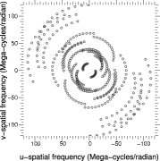
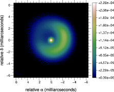
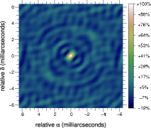
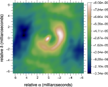
Figure 2: Top left: $(u,v)$ coverage. Top right: observed object. Bottom left: dirty beam. Bottom right: dirty image. Object model and $(u,v)$ coverage are from the 2004’ Beauty Contest [16].

III-B Inverse Problem Approach

Since many Fourier frequencies are not measured, fitting the data alone does not uniquely define the sought image. Such an ill-posed problem can be solved by an inverse problem approach [17] by imposing a priori constraints to select a unique image among all those which are consistent with the data. The requirements for the priors are that they must help to smoothly interpolate voids in the $(u,v)$ coverage while avoiding high frequencies beyond the diffraction limit. Without loss of generality, we assume that these constraints are monitored by a penalty function $f_{\mathsf{prior}}(\boldsymbol{x})$ which measures the agreement of the image with the priors: the lower $f_{\mathsf{prior}}(\boldsymbol{x})$, the better the agreement. In inverse problem framework, $f_{\mathsf{prior}}(\boldsymbol{x})$ is termed as the regularization. Then the parameters $\boldsymbol{x}^{+}$ of the image which best matches the priors while fitting the data are obtained by solving a constrained optimization problem:

$$\boldsymbol{x}^{+}=\mathop{\operator@font arg\,min}\limits f_{\mathsf{prior}}(\boldsymbol{x})\,,\ \text{subject to:\ }\mathbf{A}\cdot\boldsymbol{x}=\boldsymbol{y}\,.$$ (21)

Other strict constraints may apply. For instance, assuming the image brightness distribution must be positive and normalized, the feasible set is:

$$\mathcal{X}=\{\boldsymbol{x}\in\mathbb{R}^{N};\boldsymbol{x}\geq 0,\sum_{n}x_{n}=1\}$$ (22)

where $\boldsymbol{x}\geq 0$ means: $\forall n$, $x_{n}\geq 0$. Besides, due to noise and model approximations, there is some expected discrepancy between the model and actual data. As for the priors, the distance of the model to the data can be measured by a penalty function $f_{\mathsf{data}}(\boldsymbol{x})$. We then require that, to be consistent with the data, an image must be such that $f_{\mathsf{data}}(\boldsymbol{x})\leq\eta_{\mathsf{data}}$ where $\eta_{\mathsf{data}}$ is set according to the level of errors:

$$\boldsymbol{x}^{+}=\mathop{\operator@font arg\,min}\limits_{\boldsymbol{x}\in\mathcal{X}}f_{\mathsf{prior}}(\boldsymbol{x})\,,\ \text{subject to:\ }f_{\mathsf{data}}(\boldsymbol{x})\leq\eta_{\mathsf{data}}\,.$$ (23)

The Lagrangian of this constrained optimization problem can be written as:

$$\mathcal{L}(\boldsymbol{x};\ell)=f_{\mathsf{prior}}(\boldsymbol{x})+\ell\,\Bigl{(}f_{\mathsf{data}}(\boldsymbol{x})-\eta_{\mathsf{data}}\Bigr{)}$$ (24)

where $\ell$ is the Lagrange multiplier associated to the inequality constraint $f_{\mathsf{data}}(\boldsymbol{x})\leq\eta_{\mathsf{data}}$. If the constraint is active, then $\ell>0$ and $f_{\mathsf{data}}(\boldsymbol{x})=\eta_{\mathsf{data}}$ [18]. Dropping the constant $\eta_{\mathsf{data}}$ which does not depend on $\boldsymbol{x}$, the solution is obtained by solving either of the following problems:

$$\boldsymbol{x}^{+} =\mathop{\operator@font arg\,min}\limits_{\boldsymbol{x}\in\mathcal{X}}\{f_{\mathsf{prior}}(\boldsymbol{x})+\ell\,f_{\mathsf{data}}(\boldsymbol{x})\}$$

$$=\mathop{\operator@font arg\,min}\limits_{\boldsymbol{x}\in\mathcal{X}}f(\boldsymbol{x};\mu)\,,$$

where

$$f(\boldsymbol{x};\mu)=f_{\mathsf{data}}(\boldsymbol{x})+\mu\,f_{\mathsf{prior}}(\boldsymbol{x})$$ (25)

is the penalty function and $\mu=1/\ell>0$ has to be tuned to match the constraint $f_{\mathsf{data}}(\boldsymbol{x})=\eta_{\mathsf{data}}$. Hence we can equivalently consider that we are solving the problem of maximizing the agreement of the model with the data subject to the constraint that the priors be below a preset level:

$$\boldsymbol{x}^{+}=\mathop{\operator@font arg\,min}\limits_{\boldsymbol{x}\in\mathcal{X}}f_{\mathsf{data}}(\boldsymbol{x})\,,\ \text{subject to:\ }f_{\mathsf{prior}}(\boldsymbol{x})\leq\eta_{\mathsf{prior}}\,.$$ (26)

For convex penalties and providing that the Lagrange multipliers ($\mu$ and $\ell$) and the thresholds ($\eta_{\mathsf{data}}$ and $\eta_{\mathsf{prior}}$) are set consistently, the image restoration is achieved by solving either of the problems in Eq. (23), Eq. (26) or by minimizing the penalty function in Eq. (25). However, choosing which of these particular problems to solve can be a deciding issue for the efficiency of the method. For instance, if $f_{\mathsf{data}}(\boldsymbol{x})$ and $f_{\mathsf{prior}}(\boldsymbol{x})$ are both smooth functions, direct minimization of $f(\boldsymbol{x};\mu)$ in Eq. (25) can be done by using general purpose optimization algorithms [18] but requires to know the value of the Lagrange multiplier. If the penalty functions are not smooth or if one wants to have the Lagrange multiplier automatically tuned given $\eta_{\mathsf{data}}$ or $\eta_{\mathsf{prior}}$, specific algorithms must be devised. As we will see in the following, specifying the image reconstruction as a constrained optimization problem provides a very general framework suitable to describe most existing methods; it however hides important algorithmic details about the strategy to search the solution. In the remaining of this section, we first derive expressions of the data penalty terms and, then, the various regularizations that have been considered for image reconstruction in interferometry.

III-C Distance to the Data

The $\ell_{2}$ norm is a simple means to measure the consistency of the model image with the data:

$$f_{\mathsf{data}}(\boldsymbol{x})=\left\|\boldsymbol{y}-\mathbf{A}\cdot\boldsymbol{x}\right\|^{2}_{2}\,.$$ (27)

However, to account for correlations and for the inhomogeneous quality of the measurements, the distance to the data has to be defined according to the statistics of the errors $\boldsymbol{e}=\boldsymbol{y}-\mathbf{A}\cdot\boldsymbol{x}$ given the image model. Assuming Gaussian statistics, this leads to:

$$f_{\mathsf{data}}(\boldsymbol{x})=(\boldsymbol{y}-\mathbf{A}\cdot\boldsymbol{x})^{\mathrm{T}}\cdot{\mathbf{W}}_{\mathsf{err}}\cdot(\boldsymbol{y}-\mathbf{A}\cdot\boldsymbol{x})\,,$$ (28)

where the weighting matrix ${\mathbf{W}}_{\mathsf{err}}={\mathbf{C}}_{\mathsf{err}}^{-1}$ is the inverse of the covariance matrix of the errors. There is a slight issue because we are dealing with complex values. Since complex numbers are just pairs of reals, complex valued vectors (such as $\boldsymbol{y}$, $\boldsymbol{e}$ and $\mathbf{A}\cdot\boldsymbol{x}$) can be flattened into ordinary real vectors (with doubled size) to use standard linear algebra notation and define the covariance matrix as ${\mathbf{C}}_{\mathsf{err}}=\langle\boldsymbol{e}\cdot\boldsymbol{e}^{\mathrm{T}}\rangle$. This is what is assumed in Eq. (28).

There are some possible simplifications. For instance, the complex visibilities are measured independently, hence the weighting matrix ${\mathbf{W}}_{\mathsf{err}}$ is block diagonal with $2\times 2$ blocks. Furthermore, if the real and imaginary parts of a given measured complex visibility are uncorrelated and have the same variance, then $f_{\mathsf{data}}$ takes a simple form:

$$f_{\mathsf{data}}(\boldsymbol{x})=\sum_{\ell}w_{\ell}\,\left|{{y}_{\ell}}-(\mathbf{A}\cdot\boldsymbol{x})_{\ell}\right|^{2}\,,$$ (29)

where the weights are given by:

$$w_{\ell}=\mathop{\operator@font Var}\nolimits\left(\mathop{\operator@font Re}\nolimits\left({{y}_{\ell}}\right)\right)^{-1}=\mathop{\operator@font Var}\nolimits\left(\mathop{\operator@font Im}\nolimits\left({{y}_{\ell}}\right)\right)^{-1}\,.$$ (30)

This expression of $f_{\mathsf{data}}(\boldsymbol{x})$, popularized by Goodman [19], is very commonly used in radio-interferometry.

Real data may however have different statistics. For instance, the OI-FITS file exchange format for optical interferometric data assumes that the amplitude and the phase of complex data (complex visibility or triple product) are independent [20]. The thick lines in Fig. 3 display the isocontours of the corresponding log-likelihood which forms a non-convex valley in the complex plane. Assuming Goodman statistics would yield circular isocontours in this figure and is obviously a bad approximation of the true criterion in that case. To improve on the Goodman model while avoiding non-convex criteria, Meimon et al. [14] have proposed quadratic convex approximations of the true log-likelihood (see Fig. 3) and have shown that their so-called local approximation yields the best results, notably when dealing with low signal to noise data. For a complex datum ${{y}_{\ell}}=\rho_{\ell}\,\exp(\mathrm{i}\,\varphi_{\ell})$, their local quadratic approximation writes:

$$f_{\mathsf{data}}(\boldsymbol{x})=\sum_{\ell}\left\{\frac{\mathop{\operator@font Re}\nolimits\left(e_{\ell}\,\mathrm{e}^{-\mathrm{i}\,\varphi_{\ell}}\right)^{2}}{\sigma^{2}_{/\!/,\ell}}+\frac{\mathop{\operator@font Im}\nolimits\left(e_{\ell}\,\mathrm{e}^{-\mathrm{i}\,\varphi_{\ell}}\right)^{2}}{\sigma^{2}_{\perp,\ell}}\right\}$$ (31)

where $\boldsymbol{e}=\boldsymbol{y}-\mathbf{A}\cdot\boldsymbol{x}$ denotes the complex residuals and the variances along and perpendicular to the complex datum vector are:

$$\sigma^{2}_{/\!/,\ell} =\mathop{\operator@font Var}\nolimits(\rho_{\ell})$$ (32)

$$\sigma^{2}_{\perp,\ell} =\rho_{\ell}^{2}\,\mathop{\operator@font Var}\nolimits(\varphi_{\ell})\,.$$ (33)

The Goodman model is retrieved when $\rho_{\ell}^{2}\,\mathop{\operator@font Var}\nolimits(\varphi_{\ell})=\mathop{\operator@font Var}\nolimits(\rho_{\ell})$.

Figure 3: Convex quadratic approximations of complex data. Thick lines: isocontours of the log-likelihood $f_{\mathsf{data}}$ (at 1, 2 and 3 rms levels) for a complex datum with independent amplitude and phase. Dashed lines: isocontours for the global quadratic approximation. Thin lines: isocontours for the local quadratic approximation.

III-D Maximum Entropy Methods

Maximum entropy methods (MEM) are based on the 1950s work of Jaynes on information theory; the underlying idea is to obtain the least informative image which is consistent with the data [21]. This amounts to minimizing a criterion like the one in Eq. (25) with $f_{\mathsf{prior}}(\boldsymbol{x})=-S(\boldsymbol{x})$ where the entropy $S(\boldsymbol{x})$ measures the informational contents of the image $\boldsymbol{x}$. In this framework, $f_{\mathsf{prior}}(\boldsymbol{x})$ is sometimes called negentropy. Among all the expressions considered for the negentropy of an image, one of the most popular is [22]:

$$f_{\mathsf{prior}}(\boldsymbol{x})=\sum_{j}\left[x_{j}\,\log(x_{j}/\bar{x}_{j})-x_{j}+\bar{x}_{j}\right]$$ (34)

with $\bar{\boldsymbol{x}}$ the default image; that is, the one which would be recovered in the absence of any data. Back to information theory, this expression is similar to the Kullback-Leibler divergence between $\boldsymbol{x}$ and $\bar{\boldsymbol{x}}$ (with additional terms that cancel for normalized distributions). The default image $\bar{\boldsymbol{x}}$ can be taken as being a flat image, an image previously restored, an image of the same object at a lower resolution, etc. Narayan & Nityananda [23] reviewed maximum entropy methods for radio-interferometry imaging and compared the other forms of the negentropy that have been proposed. They argued that only non-quadratic priors can interpolate missing Fourier data and noted that such penalties also forbid negative pixel values. The fact that there is no need to explicitly impose positivity is sometimes put forward by the proponents of these methods.

MEM penalties are usually separable, which means that they do not depend on the ordering of the pixels. To explicitly enforce some correlation between close pixels in the sought image $\boldsymbol{x}$ (hence, some smoothness), the prior can be chosen to depend on $\boldsymbol{x}$. For instance: $\bar{\boldsymbol{x}}=\mathbf{P}\cdot\boldsymbol{x}$ where $\mathbf{P}$ is some averaging or smoothing linear operator. This type of floating prior has been used to loosely enforce constraints such as radial symmetry [24]. Alternatively, an intrinsic correlation function (ICF) can be explicitly introduced by a convolution kernel to impose the correlation structure of the image [25].

Minimizing the joint criterion in Eq. (25) with entropy regularization has a number of issues as the problem is highly non-linear and as the number of unknowns is very large (as many as there are pixels). Various methods have been proposed, but the most effective algorithm [26] seeks for the solution by a non-linear optimization in a local sub-space of search directions with the Lagrange multiplier $\mu$ tuned on the fly to match the constraint that $f_{\mathsf{data}}(\boldsymbol{x})=\eta_{\mathsf{data}}$.

III-E Other Prior Penalties

Bayesian arguments can be invoked to define other types of regularization. For instance, assuming that the pixels have a Gaussian distribution leads to quadratic penalties such as:

$$f_{\mathsf{prior}}(\boldsymbol{x})=(\boldsymbol{x}-\bar{\boldsymbol{x}})^{\mathrm{T}}\cdot{\mathbf{C}}_{\mathsf{prior}}^{-1}\cdot(\boldsymbol{x}-\bar{\boldsymbol{x}})$$ (35)

with ${\mathbf{C}}_{\mathsf{prior}}$ the prior covariance and $\bar{\boldsymbol{x}}$ the prior solution. Tikhonov’s regularization [27], $f_{\mathsf{prior}}(\boldsymbol{x})=\|\boldsymbol{x}\|^{2}_{2}$, is the simplest of these penalties. By Parseval’s theorem, this regularization favors zeroes for unmeasured frequencies, it is therefore not recommended for image reconstruction in interferometry. Yet, this does not rule out all quadratic priors. For instance, compactness is achieved by a very simple quadratic penalty:

$$f_{\mathsf{prior}}(\boldsymbol{x})=\sum_{n}w^{\mathsf{prior}}_{n}\,x_{n}^{2}\,,$$ (36)

where the weights are increasing with the distance to the center of the image thus favoring structures concentrated within this part of the image. Under strict normalization constraint and in the absence of any data, the default image given by this prior is $\bar{x}_{n}\propto 1/w^{\mathsf{prior}}_{n}$ where the factor comes from the normalization requirement [28]. Although simple, this regularizer, coupled with the positivity constraint, can be very effective as shown by Fig. 4b. Indeed, smooth Fourier interpolation follows from the compactness of the brightness distribution which is imposed by $f_{\mathsf{prior}}(\boldsymbol{x})$ in Eq. (36) and by the positivity as it plays the role of a floating support.

Other prior penalties commonly used in image restoration methods can be useful for interferometry. For instance, edge-preserving smoothness is achieved by:

$$f_{\mathsf{prior}}(\boldsymbol{x})=\sum_{n_{1},n_{2}}\sqrt{\epsilon^{2}+|\nabla\boldsymbol{x}|_{n_{1},n_{2}}^{2}}$$ (37)

where $\epsilon>0$ is a chosen threshold and $|\nabla\boldsymbol{x}|^{2}$ is the squared magnitude of the spatial gradient of the image:

$$|\nabla\boldsymbol{x}|_{n_{1},n_{2}}^{2}=(x_{n_{1}+1,n_{2}}-x_{n_{1},n_{2}})^{2}+(x_{n_{1},n_{2}+1}-x_{n_{1},n_{2}})^{2}\,.$$

The penalization in Eq. (37) behaves as a quadratic (resp. linear) function where the magnitude of the spatial gradient is small (resp. large) compared to $\epsilon$. Thus reduction of small local variations without penalizing too much strong sharp features is achieved by this regularization. In the limit $\epsilon\rightarrow 0$, edge-preserving smoothness behaves like total variation [29] which has proved successful in imposing sparsity.

III-F Clean method

Favoring images with a limited number of significant pixels is a way to avoid the degeneracies of image reconstruction from sparse Fourier coefficients. This could be formally done by searching for the least $\ell_{0}$-norm image consistent with the data; hence using $f_{\mathsf{prior}}(\boldsymbol{x})=\|\boldsymbol{x}\|_{0}$. However, due to the number of parameters, minimizing the resulting mixed criterion is a combinatorial problem which is too difficult to solve directly. Clean algorithm [30, 31] implements a matching pursuit strategy to attempt to find this kind of solution. The method proceeds iteratively as follows. Given the data in the form of a dirty image, the location of the brightest point source that best explains the data is searched. The model image is then updated by a fraction of the intensity of this component, and this fraction times the dirty beam is subtracted from the dirty image. The procedure is repeated for the new residual dirty image which is searched for evidence of another point-like source. When the level of the residuals becomes smaller than a given threshold set from the noise level, the image is convolved with the clean beam (usually a Gaussian shaped PSF) to set the resolution according to the extension of the $(u,v)$ coverage. Once most point sources have been removed, the residual dirty image is essentially due to the remaining extended sources which may be smooth enough to be insensitive to the convolution by the dirty beam. Hence adding the residual dirty image to the clean image produces a final image consisting in compact sources (convolved by the clean beam) plus smooth extended components. Although designed for point sources, Clean works rather well for extended sources and remains one of the preferred methods in radio-interferometry.

It has been demonstrated that the matching pursuit part of Clean is equivalent to an iterative deconvolution with early stopping [32] and that it is an approximate algorithm for obtaining the image of minimum total flux consistent with the observations [33]. Hence, under the non-negativity constraint, this would, at best, yield the least $\ell_{1}$-norm image consistent with the data. This objective is supported by recent results in Compressive Sensing [34] showing that, in most practical cases, regularization by the $\ell_{1}$-norm of $\boldsymbol{x}$ enforces the sparsity of the solution. However, the matching pursuit strategy implemented by Clean is slow, it has some instabilities and it is known to be sub-optimal [33].

III-G Other methods

This section briefly reviews other image reconstruction methods applied in astronomical interferometry.

III-G1 Multi-resolution

These methods aim at reconstructing images with different scales. They basically rely on recursive decomposition of the image in low and high frequencies. Multi-resolution Clean [35] first reconstructs an image of the broad emission and then iteratively updates this map at full resolution as in the original Clean algorithm. This approach has been generalized by using a wavelet expansion to describe the image — which could be formally expressed in terms of Eq. (13) — and achieved multi-resolution deconvolution by a matching pursuit algorithm applied to the wavelet coefficients and such that the solution satisfies positivity and support constraints [36]. The multi-scale Clean algorithm [37] explicitly describes the image as a sum of components with different scales and makes use of a weighted matching pursuit algorithm to search for the scale and position of each image update. The main advantages of multi-scale Clean are its ability to leave very few structures in the final residuals and to correctly estimate the total flux of the observed object. This method is widely used in radio-astronomy and is part of standard data processing packages [38]. In the context of MEM, the multi-channel maximum entropy image reconstruction method [39] introduces a multi-scale structure in the image by means of different intrinsic correlation functions [25]. The reconstructed image is then the sum of several extended sources with different levels of correlation. This approach was extended by using a pyramidal image decomposition [40] or wavelet expansions [41, 42].

III-G2 Wipe method

The Wipe method [10] is a regularized fit of the interferometric data under positivity and support constraints. The model image is given by Eq. (13) using an equally-spaced grid and the effective resolution is explicitly set by the basis function $b(\boldsymbol{\theta})$, the so-called neat beam, with an additional penalty to avoid super resolution. The image parameters are the ones that minimize:

$$f_{\mathsf{Wipe}}(\boldsymbol{x})=\sum_{\ell}w_{\ell}\,|\hat{b}_{\ell}\,{{y}_{\ell}}-(\mathbf{A}\cdot\boldsymbol{x})_{\ell}|^{2}+\sum_{k,|\nu_{k}|>\nu_{\mathsf{eff}}}|(\mathbf{F}\cdot\boldsymbol{x})_{k}|^{2}$$

with $\boldsymbol{y}$ the calibrated complex visibility data, $\hat{b}_{\ell}$ the Fourier transform of the neat beam at the spatial frequency of datum ${{y}_{\ell}}$, $\nu_{\mathsf{eff}}\gtrsim\mathrm{sup}_{\nu\in\mathcal{L}}|\nu|$ an effective cutoff frequency, $\mathbf{F}$ the Fourier transform operator, $\mathbf{A}$ the model matrix given by Eq. (18) accounting for the sub-sampled Fourier transform and the neat beam, and $w_{\ell}=1/(\sigma^{2}_{\ell}\,\sum_{\ell^{\prime}}\sigma^{-2}_{\ell^{\prime}})$ where $\sigma^{2}_{\ell}=|\hat{b}_{\ell}|^{2}\,\mathop{\operator@font Var}\nolimits({{y}_{\ell}})$ assuming the Goodman approximation. In the criterion minimized by Wipe, one can identify the distance of the model to the data and a regularization term. There is no hyper-parameter to tune the level of this latter term. The optimization is done by a conjugate gradient search with a stopping criterion derived from the analysis of the conditioning of the problem. This analysis is built up during the iterations.

III-G3 Bi-model method

The case of an image model explicitly mixing extended source and point sources has also been addressed [43, 44] and more recently [15]. The latter have considered an image $\boldsymbol{x}=\boldsymbol{x}_{\mathsf{e}}+\boldsymbol{x}_{\mathsf{p}}$ made of two maps: $\boldsymbol{x}_{\mathsf{e}}$ for extended structures and $\boldsymbol{x}_{\mathsf{p}}$ for point-like components. The maps $\boldsymbol{x}_{\mathsf{e}}$ and $\boldsymbol{x}_{\mathsf{p}}$ are respectively regularized by imposing smoothness and sparsity. With additional positivity and, optionally, support constraints, it turns out that the two kinds of regularization can be implemented by quadratic penalties. Their method amounts to minimize:

$$f_{\mathsf{mix}}(\boldsymbol{x}_{\mathsf{e}},\boldsymbol{x}_{\mathsf{p}}) =\left\|\boldsymbol{y}-\mathbf{A}\cdot(\boldsymbol{x}_{\mathsf{e}}+\boldsymbol{x}_{\mathsf{p}})\right\|^{2}+\lambda_{\mathsf{s}}\,\boldsymbol{c}^{\mathrm{T}}\cdot\boldsymbol{x}_{\mathsf{p}}$$

$$\hskip 10.00002pt+\epsilon_{\mathsf{s}}\,\|\boldsymbol{x}_{\mathsf{p}}\|^{2}+\lambda_{\mathsf{c}}\,\|\boldsymbol{x}_{\mathsf{e}}\|_{{\mathbf{C}}_{\mathsf{prior}}}^{2}+\epsilon_{\mathsf{m}}\,(\boldsymbol{c}^{\mathrm{T}}\cdot\boldsymbol{x}_{\mathsf{e}})^{2}\,$$

with $\|\boldsymbol{x}_{\mathsf{e}}\|^{2}_{{\mathbf{C}}_{\mathsf{prior}}}$ a local finite difference norm similar to Eq. (35), and $\boldsymbol{c}$ a vector with all components set to one, hence: $\boldsymbol{c}^{\mathrm{T}}\cdot\boldsymbol{x}=\sum_{n}x_{n}$. There are 4 tuning parameters for the regularization terms: $\lambda_{\mathsf{s}}\geq 0$ and $\epsilon_{\mathsf{s}}>0$ control the sparsity of $\boldsymbol{x}_{\mathsf{p}}$, $\lambda_{\mathsf{c}}>0$ controls the level of smoothness in the extended map $\boldsymbol{x}_{\mathsf{e}}$, and $\epsilon_{\mathsf{m}}>0$ (or $\epsilon_{\mathsf{m}}\geq 0$ if there is a support constraint) insures strict convexity of the regularization with respect to $\boldsymbol{x}_{\mathsf{e}}$. Circulant approximations are used to implement a very fast minimization of $f_{\mathsf{mix}}(\boldsymbol{x}_{\mathsf{e}},\boldsymbol{x}_{\mathsf{p}})$ under the constraints that $\boldsymbol{x}_{\mathsf{e}}\geq 0$ and $\boldsymbol{x}_{\mathsf{p}}\geq 0$ [15].

III-H Self-Calibration

When the OTF cannot be calibrated (e.g. there is no reference or the OTF is significantly varying due to the turbulence), the problem is not only to derive the image parameters $\boldsymbol{x}$, but also the unknown complex throughputs $\boldsymbol{g}$. As there is no correlation between the throughputs and the observed object, the inverse approach leads to solve:

$$(\boldsymbol{x},\boldsymbol{g})^{+} =\mathop{\operator@font arg\,min}\limits_{\boldsymbol{x}\in\mathcal{X},\boldsymbol{g}}\left\{f_{\mathsf{data}}(\boldsymbol{x},\boldsymbol{g})+\mu_{\mathsf{img}}\,f_{\mathsf{prior}}^{\mathsf{img}}(\boldsymbol{x})\right.$$

$$\hskip 87.00009pt\quad\left.{+}\>\mu_{\mathsf{gain}}\,f_{\mathsf{prior}}^{\mathsf{gain}}(\boldsymbol{g})\right\}$$ (38)

with $\mu_{\mathsf{img}}\,f_{\mathsf{prior}}^{\mathsf{img}}(\boldsymbol{x})$ and $\mu_{\mathsf{gain}}\,f_{\mathsf{prior}}^{\mathsf{gain}}(\boldsymbol{g})$ the regularization terms for the image parameters and for the complex throughputs. The latter can be derived from prior statistics about the turbulence [5]. In principle, global optimization should be required to minimize the non-convex criterion in Eq. (III-H). Fortunately, a simpler strategy based on alternate minimization with respect to $\boldsymbol{x}$ only and then with respect to $\boldsymbol{g}$ only has proved effective to solve this problem. This method has been called self-calibration because it uses the current estimate of the sought image as a reference source to calibrate the throughputs. The algorithm begins with an initial image $\boldsymbol{x}^{[0]}$ and repeats until convergence the following steps (starting with $n=1$ and incrementing $n$ after each iteration):

1. Self-calibration step. Given the image $\boldsymbol{x}^{[n-1]}$, find the best complex throughputs $\boldsymbol{g}^{[n]}$ by solving:

   $$\boldsymbol{g}^{[n]}=\mathop{\operator@font arg\,min}\limits_{\boldsymbol{g}}\left\{f_{\mathsf{data}}\bigl{(}\boldsymbol{x}^{[n-1]},\boldsymbol{g}\bigr{)}+\mu_{\mathsf{gain}}\,f_{\mathsf{prior}}^{\mathsf{gain}}(\boldsymbol{g})\right\}\,.$$

2. Image reconstruction step. Apply image reconstruction algorithm to recover a new image estimate given the data and the complex throughputs:

   $$\boldsymbol{x}^{[n]}=\mathop{\operator@font arg\,min}\limits_{\boldsymbol{x}}\left\{f_{\mathsf{data}}\bigl{(}\boldsymbol{x},\boldsymbol{g}^{[n]}\bigr{)}+\mu_{\mathsf{img}}\,f_{\mathsf{prior}}^{\mathsf{img}}(\boldsymbol{x})\right\}\,.$$

Note that any image reconstruction algorithm described previously can be used in the second step of the method. The criterion in Eq. (III-H) being non-convex, the solution should depend on the initialization. Yet, this does not appear to be an issue in practice even if simple local optimization methods are used to solve the self-calibration step (such as the one recently proposed by Lacour et al. [45]).

Self-calibration was initially proposed by Readhead & Wilkinson [46] to derive missing Fourier phase information from phase closure data, and the technique was later improved by Cotton [47]. Schwab [48] was the first to solve the problem by explicitly minimizing a non-linear criterion similar to $f_{\mathsf{data}}(\boldsymbol{x},\boldsymbol{g})$ in Eq. (29). Schwab’s approach was further improved by Cornwell & Wilkinson [49] who introduced priors for the complex gains, that is, the term $\mu_{\mathsf{gain}}\,f_{\mathsf{prior}}^{\mathsf{gain}}(\boldsymbol{g})$ in the global penalty. However, for most authors, no priors about the throughputs are assumed, hence $\mu_{\mathsf{gain}}=0$.

Self-calibration is a particular case of the blind, or myopic, deconvolution methods [50] that have been developed to improve the quality of blurred images when the point spread function (PSF) is unknown. Indeed, when the PSF can be completely described by phase aberrations in the pupil plane, blind deconvolution amounts to solving the same problem as self-calibration [51].

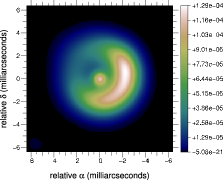
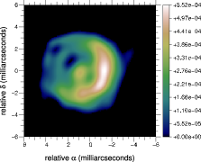
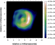
Figure 4: Image reconstruction with various types of regularization. From top-left to bottom-right: (a) original object smoothed to the resolution of the interferometer ($\mathrm{FWHM}\sim 15\,\mathrm{mas}$); (b) reconstruction with a quadratic regularization given by Eq. (36) and which imposes a compact field of view; (c) reconstruction with edge-preserving regularization as in Eq. (37); (d) reconstruction with maximum entropy regularization as in Eq. (34). All reconstructions by algorithm MiRA and from the power spectrum and the phase closures.

IV Image Reconstruction from Non-Linear Data

At optical wavelengths, the complex visibilities (whether they are calibrated or not) are not directly measurable, the available data (cf. Section II) are the power spectrum, the bispectrum and/or the phase closure. Image reconstruction algorithms can be designed following the same inverse problem approach as previously. In particular, the regularization can be implemented by the same $f_{\mathsf{prior}}$ penalties as in Section III. However, the direct model of the data is now non-linear and specific expressions to implement $f_{\mathsf{data}}$ have to be derived. The non-linearity has also some incidence on the optimization strategy.

IV-A Data Penalty

The power spectrum, the bispectrum, and the phase closure data have non-Gaussian statistics: the power spectrum is a positive quantity, the phase closure is wrapped in $(-\pi,+\pi]$, etc. Most algorithms however make use of quadratic penalties with respect to the measurements which implies Gaussian statistics in a Bayesian framework. Another assumption generally made is the independence of the measurements, which leads to separable penalties. Under such approximations, the penalty with respect to the power spectrum data writes:

$$f_{\mathsf{data}}^{\mathsf{ps}}(\boldsymbol{x})=\sum_{m,j_{1}<j_{2}}\frac{\left(S_{j_{1},j_{2},m}^{\mathsf{data}}-S_{j_{1},j_{2},m}^{\mathsf{model}}(\boldsymbol{x})\right)^{2}}{\mathop{\operator@font Var}\nolimits\left(S_{j_{1},j_{2},m}^{\mathsf{data}}\right)}\,,$$ (39)

with $S_{j_{1},j_{2},m}^{\mathsf{model}}(\boldsymbol{x})=|\hat{I}(\boldsymbol{\nu}_{j_{1},j_{2},m})|^{2}$ the model of the power spectrum. For the penalty with respect to the bispectrum data, there is the additional difficulty to deal with complex data. The Goodman approximation [19] yields:

$$f_{\mathsf{data}}^{\mathsf{bisp}}(\boldsymbol{x})=\sum_{m,j_{1}<j_{2}<j_{3}}w^{\mathsf{bisp}}_{j_{1},j_{2},j_{3},m}\,\left|B_{j_{1},j_{2},j_{3},m}^{\mathsf{data}}-B_{j_{1},j_{2},j_{3},m}^{\mathsf{model}}(\boldsymbol{x})\right|^{2}$$ (40)

with $B_{j_{1},j_{2},j_{3},m}^{\mathsf{model}}(\boldsymbol{x})=\hat{I}(\boldsymbol{\nu}_{j_{1},j_{2},m})\,\hat{I}(\boldsymbol{\nu}_{j_{2},j_{3},m})\,\hat{I}(\boldsymbol{\nu}_{j_{3},j_{1},m})$ the model of the bispectrum and weights derived from the variance of the bispectrum data. An expression similar to that in Eq. (31) can be derived for bispectrum data with independent modulus and phase errors. To account for phase wrapping, Haniff [52] proposed to define the penalty with respect to the phase closure data as:

$$f_{\mathsf{data}}^{\mathsf{cl}}(\boldsymbol{x})=\sum_{m,j_{1}<j_{2}<j_{3}}\frac{\mathop{\operator@font arc}\nolimits^{2}\left(\beta_{j_{1},j_{2},j_{3},m}^{\mathsf{data}}-\beta_{j_{1},j_{2},j_{3},m}^{\mathsf{model}}(\boldsymbol{x})\right)}{\mathop{\operator@font Var}\nolimits\left(\beta_{j_{1},j_{2},j_{3},m}^{\mathsf{data}}\right)}$$ (41)

with $\beta_{j_{1},j_{2},j_{3},m}^{\mathsf{model}}(\boldsymbol{x})=\varphi(\boldsymbol{\nu}_{j_{1},j_{2},m})+\varphi(\boldsymbol{\nu}_{j_{2},j_{3},m})+\varphi(\boldsymbol{\nu}_{j_{3},j_{1},m})$ the model of the phase closure. This penalty is however not continuously differentiable with respect to $\boldsymbol{x}$, which can prevent the convergence of optimization algorithms. This problem can be avoided by using the complex phasors [53]:

$$f_{\mathsf{data}}^{\mathsf{cl}}(\boldsymbol{x})=\sum_{m,j_{1}<j_{2}<j_{3}}\frac{\bigl{|}\mathrm{e}^{\mathrm{i}\,\beta_{j_{1},j_{2},j_{3},m}^{\mathsf{data}}}-\mathrm{e}^{\mathrm{i}\,\beta_{j_{1},j_{2},j_{3},m}^{\mathsf{model}}(\boldsymbol{x})}\bigr{|}^{2}}{\mathop{\operator@font Var}\nolimits\left(\beta_{j_{1},j_{2},j_{3},m}^{\mathsf{data}}\right)}\,,$$ (42)

which is approximately equal to the penalty in Eq. (41) in the limit of small phase closure errors.

Depending on which set of data is available, and assuming that the different types of data have statistically independent errors, the total penalty with respect to the data is simply a sum of some of the penalties given by equations (39)–(42). For instance, to fit the power spectrum and the phase closure data:

$$f_{\mathsf{data}}(\boldsymbol{x})=f_{\mathsf{data}}^{\mathsf{ps}}(\boldsymbol{x})+f_{\mathsf{data}}^{\mathsf{cl}}(\boldsymbol{x})\,.$$ (43)

IV-B Image Reconstruction Algorithms

We describe here the image reconstruction methods used with some success on realistic optical interferometric data in astronomy and which can be considered as ready to process real data. In addition to cope with sparse Fourier data, these methods were specifically designed to tackle the non-linear direct model, to account for the particular statistics of the data [14] and to handle the new data format [20]. These image reconstruction methods can all be formally described in terms of a criterion to optimize, perhaps under some strict constraints, and an optimization strategy. Some of these algorithms have clearly inherited from methods previously developed: BSMEM [54], the Building-Block Method [9] and Wisard [55] are respectively related to MEM (cf. Section III-D), Clean (cf. Section III-F) and self-calibration (cf. Section III-H).

1) BSMEM algorithm [54, 56] makes use of a Maximum Entropy Method (cf. Section III-D) to regularize the problem of image restoration from the measured bispectrum (hence its name). The improved BSMEM version [56] uses the Gull and Skilling entropy, see Eq. (34), and a likelihood term with respect to the complex bispectrum which assumes independent Gaussian noise statistics for the amplitude and phase of the measured bispectrum. The optimization engine is MemSys which implements the strategy proposed by Skilling & Bryan [26] and automatically finds the most likely value for the hyper-parameter $\mu$. The default image is either a Gaussian, a uniform disk, or a Dirac centered in the field of view. Because it makes no attempt to directly convert the data into complex visibilities, a strength of BSMEM is that it can handle any type of data sparsity (such as missing closures). Thus, in principle, BSMEM could be used to restore images when Fourier phase data are completely missing (see Fig. 5).

2) The Building Block Method [9] is similar to the Clean method but designed for reconstructing images from bispectrum data obtained by means of speckle or long baseline interferometry. The method proceeds iteratively to reduce a cost function $f_{\mathsf{data}}^{\mathsf{bisp}}$ equal to that in Eq. (40) with weights set to a constant or to an expression motivated by Wiener filtering. The minimization of the penalty is achieved by a matching pursuit algorithm which imposes sparsity of the solution. The image is given by the building block model in Eq.’s (13)-(14) and, at the $n$-th iteration, the new image $I^{[n]}(\boldsymbol{\theta})$ is obtained by adding a new building block at location $\boldsymbol{\theta}^{[n]}$ with a weight $\alpha^{[n]}$ to the previous image, so as to maintain the normalization:

$$I^{[n]}(\boldsymbol{\theta})=(1-\alpha^{[n]})\,I^{[n-1]}(\boldsymbol{\theta})+\alpha^{[n]}\,b(\boldsymbol{\theta}-\boldsymbol{\theta}^{[n]})\,.$$

The weight and location of the new building block is derived by minimizing the criterion $f_{\mathsf{data}}^{\mathsf{bisp}}$ with respect to these parameters. Strict positivity and support constraint can be trivially enforced by limiting the possible values for $\alpha^{[n]}$ and $\boldsymbol{\theta}^{[n]}$. To improve the convergence, the method allows to add/remove more than one block at a time. To avoid super resolution artifacts, the final image is convolved with a smoothing function with size set according to the spatial resolution of the instrument.

3) MACIM algorithm [57], for MArkov Chain IMager, aims at maximizing the posterior probability:

$$\Pr(\boldsymbol{x}|\boldsymbol{y})\propto\exp\Bigl{(}-\frac{1}{2}\,f_{\mathsf{data}}(\boldsymbol{x})-\frac{\mu}{2}\,f_{\mathsf{prior}}(\boldsymbol{x})\Bigr{)}\,.$$

MACIM implements MEM regularization and a specific regularizer which favors large regions of dark space in-between bright regions. For this latter regularization, $f_{\mathsf{prior}}(\boldsymbol{x})$ is the sum of all pixels with zero flux on either side of their boundaries. MACIM attempts to maximize $\Pr(\boldsymbol{x}|\boldsymbol{y})$ by a simulated annealing algorithm with the Metropolis sampler. Although maximizing $\Pr(\boldsymbol{x}|\boldsymbol{y})$ is the same as minimizing $f_{\mathsf{data}}(\boldsymbol{x})+\mu\,f_{\mathsf{prior}}(\boldsymbol{x})$, the use of normalized probabilities is required by the Metropolis sampler to accept or reject the image samples. In principle, simulated annealing is able to solve the global optimization problem of maximizing $\Pr(\boldsymbol{x}|\boldsymbol{y})$ but the convergence of this kind of Monte-Carlo method for such a large problem is very slow and critically depends on the parameters which define the temperature reduction law. A strict Bayesian approach can also be exploited to derive, in a statistical sense, the values of the hyper-parameters (such as $\mu$) and some a posteriori information such as the significance level of the image.

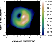
Figure 5: Image reconstruction with phase closure (left) and without any Fourier phase information (right).

4) MiRA algorithm [53] defines the sought image as the minimum of the penalty function in Eq. (25). Minimization is done by a limited variable memory method (based on BFGS updates) with bound constraints for the positivity [58]. Since this method does not implement global optimization, the image restored by MiRA depends on the initial image. MiRA is written in a modular way: any type of data can be taken into account by providing a function that computes the corresponding penalty and its gradient. For the moment, MiRA handles complex visibility, power spectrum and closure-phase data via penalty terms given by Eq. (31), Eq. (39) and Eq. (42). Also many different regularizers are built into MiRA (negentropy, quadratic or edge-preserving smoothness, compactness, total variation, etc.) and provisions are made to implement custom priors. MiRA can cope with any missing data, in particular, it can be used to restore an image given only the power spectrum (i.e. without any Fourier phase information) with at least a $180^{\circ}$ orientation ambiguity. An example of reconstruction with no phase data is shown in Fig. 5. In the case of non-sparse $(u,v)$ coverage, the problem of image reconstruction from the modulus of its Fourier transform has been addressed by Fienup [59] by means of an algorithm based on projections onto convex sets (POCS).

5) Wisard algorithm [55] recovers an image from power spectrum and phase closure data. It exploits a self-calibration approach (cf. Section III-H) to recover missing Fourier phases. Given a current estimate of the image and the phase closure data, Wisard first derives missing Fourier phase information in such a way as to minimize the number of unknowns. Then, the synthesized Fourier phases are combined with the square root of the measured power spectrum to generate pseudo complex visibility data which are fitted by the image restoration step. This step is performed by using the chosen regularization and a penalty with respect to the pseudo complex visibility data. However, to account for a more realistic approximation of the distribution of complex visibility errors, Wisard make uses of a quadratic penalty which is different from the usual Goodman approximation [14]. Taken separately, the image restoration step is a convex problem with a unique solution, the self-calibration step is not strictly convex but (like in original self-calibration method) does not seem to pose insurmountable problems. Nevertheless, the global problem is multi-modal and, at least in difficult cases, the final solution depends on the initial guess. There are many possible regularizers built into Wisard, such as the one in Eq. (36) and the edge-preserving smoothness prior in Eq. (37).

MiRA and Wisard have been developed in parallel and share some common features. They use the same optimization engine [58] and means to impose positivity and normalization [28]. They however differ in the way missing data is taken into account: Wisard takes a self-calibration (cf. Section III-H) approach to explicitly solve for missing Fourier phase information; while MiRA implicitly accounts for any lack of information through the direct model of the data[28].

All these algorithms have been compared on simulated data during Interferometric Beauty Contests [16, 60, 61]. The results of the contest were very encouraging. Although being quite different algorithms, BSMEM, the Building Block Method, MiRA and Wisard give good image reconstructions where the main features of the objects of interest can be identified in spite of the sparse $(u,v)$ coverage, the lack of some Fourier phase information and the non-linearities of the measurements. BSMEM and MiRA appear to be the most successful algorithms (they respectively won the first two and last contests).

With their tuning parameters and, for some of them, the requirement to start with an initial image, these algorithms still need some expertise to be used successfully. But this is quite manageable. For instance, the tuning of the regularization level can be derived from Bayesian considerations but can also almost be done by visual inspection of the restored image. From Fig. 6, one can see the effects of under-regularization (which yields more artifacts) and over-regularization (which yields over simplification of the image). In that case, a good regularization level is probably between $\mu=10^{5}$ and $\mu=10^{4}$ and any choice in this range would give a good image. Figure 4 shows image reconstructions from one of the data sets of the 2004’ Beauty Contest [16] and with different types of regularization. These synthesized images do not greatly differ and are all quite acceptable approximations of the reality (compare for instance with the dirty image in Fig. 2). Hence, provided that the level of the priors is correctly set, the particular choice of a given regularizer can be seen as a refinement that can be done after some reconstruction attempts with a prior that is simpler to tune. At least, the qualitative type of prior is what really matters, not the specific expression of the penalty imposing the prior.

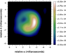
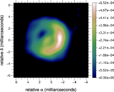
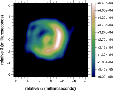
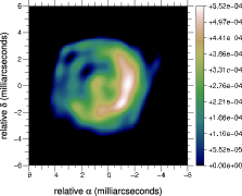
Figure 6: Image reconstruction under various regularization levels. Algorithm is MiRA with edge-preserving regularization given in Eq. (37) with $\epsilon=10^{-4}$ and $\mu=10^{6}$ (top-left), $\mu=10^{5}$ (top-right), $\mu=10^{4}$ (bottom-left) and $\mu=3\times 10^{3}$ (bottom-right).

V Discussion

The main issues in image reconstruction from interferometric data are the sparsity of the measurements (which sample the Fourier transform of the object brightness distribution) and the lack of part of the Fourier phase information. The inverse problem approach appears to be suitable to describe the most important existing algorithms in this context. Indeed, the image reconstruction methods can be stated as the minimization of a mixed criterion under some strict constraints such as positivity and normalization. Two different types of terms appear into this criterion: likelihood terms which enforce consistency of the model image with the data, and regularization terms which maintain the image close to the priors required to lever the degeneracies of the image reconstruction problem. Hence, the differences between the various algorithms lie in the kind of measurements considered, in the approximations for the direct model and for the statistics of the errors and in the prior imposed by the regularization. For non-convex criteria which occur when the OTF is unknown or when non-linear estimators are measured to overcome turbulence effects, the initial solution and the optimization strategy are also key components of the algorithms. Although global optimization is required to solve such multi-modal problems, most existing algorithms are successful whereas they only implement local optimization. These algorithms are not fully automated black boxes: at least some tuning parameters and the type of regularization are left to the user choice. Available methods are however now ready for image reconstruction from real data. Nevertheless, a general understanding of the mechanisms involved in image restoration algorithms is mandatory to correctly use these methods and to analyze possible artifacts in the synthesized images. From a technical point of view, future developments of these algorithms will certainly focus on global optimization and unsupervised reconstruction. However, to fully exploit the existing instruments, the most worthwhile tracks to investigate are multi-spectral imaging and accounting for additional data such as a low resolution image of the observed object to overcome the lack of short baselines.

Eric Thiébaut was born in Béziers, France, in 1966. He graduated from the École Normale Supérieure in 1987 and received the Ph. D. degree in Astrophysics at Université Pierre & Marie Curie (Paris VII, France), in 1994. Since 1995, he is an astronomer at the Centre de Recherche Astrophysique de Lyon. His main interests are in the fields of signal processing and image reconstruction. He made various contributions in blind deconvolution, optical interferometry and optimal detection with applications in astronomy, bio-medical imaging and digital holography.

Jean-François Giovannelli was born in Béziers, France, in 1966. He graduated from the École Nationale Supérieure de l’Électronique et de ses Applications in 1990. He received the Ph. D. degree in 1995 and the Habilitation à Diriger des Recherches in physics (signal processing) in 2005. From 1997 to 2008, he has been Assistant Professor with the Université Paris-Sud, and a Researcher with the Laboratoire des Signaux et Systèmes. He is presently Professor with the Université de Bordeaux and a Researcher with the Laboratoire d’Intégration du Matériau au Système, Équipe Signal-Image. He is interested in regularization and Bayesian methods for inverse problems in signal and image processing. His application fields essentially concern astronomical, medical, protemics and geophysical imaging.

References

- [1] A. Labeyrie, “Interference fringes obtained on VEGA with two optical telescopes,” Astrophys. J. Lett., vol. 196, p. L71, 1975.
- [2] A. Quirrenbach, “Optical Interferometry,” Annual Rev. of Astron. & Astrophys., vol. 39, p. 353, 2001.
- [3] J. Monnier, “Optical interferometry in astronomy,” Reports on Progress in Physics, vol. 66, p. 789, 2003.
- [4] G. Perrin, “VLTI Science Highlights,” in Proc. Astrophysics and Space Science: Science with the VLT in the ELT Era, 2009, p. 81.
- [5] F. Roddier, “The effects of atmospheric turbulence in optical astronomy,” in Progress In Optics, 1981, vol. 19, p. 281.
- [6] F. Delplancke, F. Derie, F. Paresce, A. Glindemann, F. Lévy, S. Lévêque, and S. Ménardi, “Prima for the VLTI - science,” Astrophys. & Space Science, vol. 286, p. 99, 2003.
- [7] J. Dainty and A. Greenaway, “Estimation of spatial power spectra in speckle interferometry,” J. Opt. Soc. Am., vol. 69, p. 786, 1979.
- [8] B. Wirnitzer, “Bispectral analysis at low light levels and astronomical speckle masking,” J. Opt. Soc. Am. A, vol. 2, p. 14, 1985.
- [9] K.-H. Hofmann and G. Weigelt, “Iterative image reconstruction from the bispectrum,” Astron. & Astrophys., vol. 278, p. 328, 1993.
- [10] A. Lannes, E. Anterrieu, and P. Maréchal, “Clean and Wipe,” Astron. & Astrophys. Suppl., vol. 123, p. 183, 1997.
- [11] D. Potts, G. Steidl, and M. Tasche, “Fast Fourier transforms for nonequispaced data: A tutorial,” in Modern Sampling Theory: Mathematics and Applications, J. Benedetto and P. Ferreira, Eds., 2001, p. 249.
- [12] A. Thompson and R. Bracewell, “Interpolation and Fourier transformation of fringe visibilities,” Astron. J., vol. 79, p. 11, 1974.
- [13] R. Sramek and F. Schwab, “Imaging,” in Synthesis Imaging in Radio Astronomy, vol. 6, 1989, p. 117.
- [14] S. Meimon, L. Mugnier, and G. Le Besnerais, “Convex approximation to the likelihood criterion for aperture synthesis imaging,” J. Opt. Soc. Am. A, vol. 22, p. 2348, 2005.
- [15] J.-F. Giovannelli and A. Coulais, “Positive deconvolution for superimposed extended source and point sources,” Astron. & Astrophys., vol. 439, p. 401, 2005.
- [16] P. Lawson, W. Cotton, C. Hummel, J. Monnier, M. Zhao, J. Young, H. Thorsteinsson, S. Meimon, L. Mugnier, G. Le Besnerais, E. Thiébaut, and P. Tuthill, “The 2004 optical/IR interferometry imaging beauty contest,” Bulletin American Astron. Soc., vol. 36, p. 1605, 2004.
- [17] A. Tarantola, Inverse Problem Theory and Methods for Model Parameter Estimation. SIAM, 2005.
- [18] J. Nocedal and S. Wright, Numerical Optimization. Springer, 2006.
- [19] J. Goodman, Statistical Optics. John Wiley & Sons, 1985.
- [20] T. Pauls, J. Young, W. Cotton, and J. Monnier, “A data exchange standard for optical (visible/IR) interferometry,” Publications of the ASP, vol. 117, p. 1255, 2005.
- [21] J. Ables, “Maximum Entropy Spectral Analysis,” Astron. & Astrophys. Suppl., vol. 15, p. 383, 1974.
- [22] S. Gull and J. Skilling, “The maximum entropy method,” in Measurement and Processing for Indirect Imaging, 1984, p. 267.
- [23] R. Narayan and R. Nityananda, “Maximum entropy image restoration in astronomy,” Annual Rev. of Astron. & Astrophys., vol. 24, p. 127, 1986.
- [24] K. Horne, “Images of accretion discs – I. The eclipse mapping method,” Monthly Notices of the RAS, vol. 213, p. 129, 1985.
- [25] S. Gull, “Developments in maximum entropy data analysis,” in Maximum Entropy and Bayesian Methods, J. Skilling, Ed., 1989, p. 53.
- [26] J. Skilling and R. Bryan, “Maximum entropy image reconstruction: general algorithm,” Monthly Notices of the RAS, vol. 211, p. 111, 1984.
- [27] A. Tikhonov and V. Arsenin, “Solution of ill-posed problems,” in Scripta Series in Mathematics, 1977.
- [28] G. Le Besnerais, S. Lacour, L. Mugnier, E. Thiébaut, G. Perrin, and S. Meimon, “Advanced imaging methods for long-baseline optical interferometry,” IEEE Journal of Selected Topics in Signal Processing, vol. 2, p. 767, 2008.
- [29] D. Strong and T. Chan, “Edge-preserving and scale-dependent properties of total variation regularization,” Inverse Problems, vol. 19, p. S165, 2003.
- [30] E. Fomalont, “Earth-rotation aperture synthesis,” Proc. IEEE: Special issue on radio and radar astronomy, vol. 61, p. 1211, 1973.
- [31] J. Högbom, “Aperture synthesis with a non-regular distribution of interferometer baselines,” Astron. & Astrophys. Suppl., vol. 15, p. 417, 1974.
- [32] U. Schwarz, “Mathematical-statistical description of the iterative beam removing technique (method CLEAN),” Astron. & Astrophys., vol. 65, p. 345, 1978.
- [33] K. Marsh and J. Richardson, “The objective function implicit in the CLEAN algorithm,” Astron. & Astrophys., vol. 182, p. 174, 1987.
- [34] E. Candes, J. Romberg, and T. Tao, “Robust uncertainty principles: exact signal reconstruction from highly incomplete frequency information,” IEEE Trans. on Information Theory, vol. 52, pp. 489– 509, 2006.
- [35] B. Wakker and U. Schwarz, “The Multi-Resolution CLEAN and its application to the short-spacing problem in interferometry,” Astron. & Astrophys., vol. 200, p. 312, 1988.
- [36] J.-L. Starck, A. Bijaoui, B. Lopez, and C. Perrier, “Image reconstruction by the wavelet transform applied to aperture synthesis,” Astron. & Astrophys., vol. 283, p. 349, 1994.
- [37] T. Cornwell, “Multiscale CLEAN deconvolution of radio synthesis images,” IEEE J. Sel. Topics Signal Process., vol. 2, p. 793, 2008.
- [38] J. Rich, W. de Blok, T. Cornwell, E. Brinks, F. Walter, I. Bagetakos, and R. Kennicutt, “Multi-Scale CLEAN: A Comparison of its Performance Against Classical CLEAN on Galaxies Using THINGS,” Astron. J., vol. 136, p. 2897, 2008.
- [39] N. Weir, “A Multi-Channel Method of Maximum Entropy Image Restoration,” in Astron. Soc. Pacific Conf.: Astronomical Data Analysis Software and Systems I, vol. 25, 1992, p. 186.
- [40] T. Bontekoe, E. Koper, and D. Kester, “Pyramid maximum entropy images of IRAS survey data,” Astron. & Astrophys., vol. 284, p. 1037, 1994.
- [41] E. Pantin and J.-L. Starck, “Deconvolution of astronomical images using the multiscale maximum entropy method,” Astron. & Astrophys. Suppl., vol. 118, p. 575, 1996.
- [42] J.-L. Starck, F. Murtagh, P. Querre, and F. Bonnarel, “Entropy and astronomical data analysis: Perspectives from multiresolution analysis,” Astron. & Astrophys., vol. 368, p. 730, 2001.
- [43] P. Magain, F. Courbin, and S. Sohy, “Deconvolution with correct sampling,” Astrophys. J., vol. 494, p. 472, 1998.
- [44] N. Pirzkal, R. Hook, and L. Lucy, “GIRA - Two Channel Photometric Restoration,” in Astron. Soc. Pacific Conf.: Astronomical Data Analysis Software and Systems IX, vol. 216, 2000, p. 655.
- [45] S. Lacour, E. Thiébaut, and G. Perrin, “High dynamic range imaging with a single-mode pupil remapping system: a self-calibration algorithm for highly redundant interferometric arrays,” Monthly Notices of the RAS, vol. 374, p. 832, 2007.
- [46] A. Readhead and P. Wilkinson, “The mapping of compact radio sources from VLBI data,” Astrophys. J., vol. 223, p. 25, 1978.
- [47] W. Cotton, “A method of mapping compact structure in radio sources using VLBI observations,” Astron. J., vol. 84, p. 1122, 1979.
- [48] F. Schwab, “Adaptive calibration of radio interferometer data,” in Proc. SPIE, vol. 231, 1980, p. 18.
- [49] T. Cornwell and P. Wilkinson, “A new method for making maps with unstable radio interferometers,” Monthly Notices of the RAS, vol. 196, p. 1067, 1981.
- [50] P. Campisi and K. Egiazarian, Eds., Blind image deconvolution: theory and applications. CRC Press, 2007.
- [51] T. Schulz, “Multiframe blind deconvolution of astronomical images,” J. Opt. Soc. Am. A, vol. 10, p. 1064, 1993.
- [52] C. Haniff, “Least-squares Fourier phase estimation from the modulo bispectrum phase,” J. Opt. Soc. Am. A, vol. 8, p. 134, 1991.
- [53] E. Thiébaut, “MiRA: an effective imaging algorithm for optical interferometry,” in proc. SPIE: Astronomical Telescopes and Instrumentation, vol. 7013, 2008, p. 70131I.
- [54] D. Buscher, “Direct maximum-entropy image reconstruction from the bispectrum,” in IAU Symp. 158: Very High Angular Resolution Imaging, 1994, p. 91.
- [55] S. Meimon, L. Mugnier, and G. Le Besnerais, “Reconstruction method for weak-phase optical interferometry,” Optics Lett., vol. 30, p. 1809, 2005.
- [56] F. Baron and J. Young, “Image reconstruction at cambridge university,” in Proc. SPIE: Astronomical Telescopes and Instrumentation, vol. 7013, 2008, p. 144.
- [57] M. Ireland, J. Monnier, and N. Thureau, “Monte-carlo imaging for optical interferometry,” in Proc. SPIE: Advances in Stellar Interferometry, vol. 6268, 2008, p. 62681T.
- [58] E. Thiébaut, “Optimization issues in blind deconvolution algorithms,” in Proc. SPIE: Astronomical Data Analysis II, vol. 4847, 2002, p. 174.
- [59] J. Fienup, “Reconstruction of an object from the modulus of its Fourier transform,” Optics Lett., vol. 3, p. 27, 1978.
- [60] P. Lawson, W. Cotton, C. Hummel, F. Baron, J. Young, S. Kraus, K.-H. Hofmann, G. Weigelt, M. Ireland, J. Monnier, E. Thiébaut, S. Rengaswamy, and O. Chesneau, “The 2006 interferometry image beauty contest,” in Proc. SPIE: Advances in Stellar Interferometry, vol. 6268, 2006, p. 62681U.
- [61] W. Cotton, J. Monnier, F. Baron, K.-H. Hofmann, S. Kraus, G. Weigelt, S. Rengaswamy, E. Thiébaut, P. Lawson, W. Jaffe, C. Hummel, T. Pauls, Henrique, P. Tuthill, and J. Young, “2008 imaging beauty contest,” in Proc. SPIE: Astronomical Telescopes and Instrumentation, vol. 7013, 2008, p. 70131N.