The Role of Intramolecular Barriers on the Glass Transition of Polymers:
Computer Simulations vs. Mode Coupling Theory

Abstract

We present computer simulations of a simple bead-spring model for polymer melts with intramolecular barriers. By systematically tuning the strength of the barriers, we investigate their role on the glass transition. Dynamic observables are analyzed within the framework of the Mode Coupling Theory (MCT). Critical nonergodicity parameters, critical temperatures and dynamic exponents are obtained from consistent fits of simulation data to MCT asymptotic laws. The so-obtained MCT $\lambda$-exponent increases from standard values for fully-flexible chains to values close to the upper limit for stiff chains. In analogy with systems exhibiting higher-order MCT transitions, we suggest that the observed large $\lambda$-values arise form the interplay between two distinct mechanisms for dynamic arrest: general packing effects and polymer-specific intramolecular barriers. We compare simulation results with numerical solutions of the MCT equations for polymer systems, within the polymer reference interaction site model (PRISM) for static correlations. We verify that the approximations introduced by the PRISM are fulfilled by simulations, with the same quality for all the range of investigated barrier strength. The numerical solutions reproduce the qualitative trends of simulations for the dependence of the nonergodicity parameters and critical temperatures on the barrier strength. In particular, the increase of the barrier strength at fixed density increases the localization length and the critical temperature. However the qualitative agreement between theory and simulation breaks in the limit of stiff chains. We discuss the possible origin of this feature.

I. INTRODUCTION

Since they do not easily crystallize, polymers are probably the most extensively studied systems in relation with the glass transition phenomenon. Having said this, their macromolecular character, and in particular chain connectivity, must not be forgotten. The most evident effect of chain connectivity is the sublinear increase of the mean squared displacement (Rouse-like) doi arising after the decaging process, in contrast to the linear regime found in non-polymeric glass-formers. Moreover, in the case of strongly entangled polymer chains, the reptation model predicts other two sublinear regimes between the Rouse and linear regimes doi ; degennes ; mcleish .

Another particular ingredient of polymers is that, apart from fast librations or methyl group rotations methylrev , every motion involves jumps over carbon-carbon rotational barriers and/or chain conformational changes. Intramolecular barriers play a decisive role in the physical properties of polymer systems. Thus, they are responsible of partial or total crystallization meyer ; vettorel . They also enhance dynamic features which are usually associated to reptation faller ; bulacu1 , which controls rheological properties mcleish . Models for semiflexible polymers are of great interest, since they can be applied to many important biopolymers such as proteins, DNA, rodlike viruses, or actin filaments bustamante ; kas ; ober . Moreover, chain stiffness seems to play an important role in the absorption behavior of polymers at interfaces semenov ; ubbink . Thus, an understandig of the role of intramolecular barriers on structural, dynamic and rheological properties of polymers is of practical as well as of fundamental interest.

In this work we investigate, by means of molecular dynamics simulations, the role of intramolecular barriers on the glass transition of polymer melts, by systematically tuning barrier strength in a simple bead-spring model. We discuss the obtained results within the framework of the Mode Coupling Theory (MCT) of the glass transition mctrev1 ; mctrev2 ; gotzebook ; reichman ; das ; gotzenewbook . We extend preliminary results reported by us in Ref. bernabei by testing a large set of predictions, including the factorization theorem and time-temperature superposition principle. A consistent set of dynamic exponents associated to asymptotic scaling laws is obtained. By increasing the barrier strength a crossover is observed for the values of the so-called $\lambda$-exponent. In the limit of fully-flexible chains $\lambda$ takes values $\sim 0.7$, characteristic of simple fluids dominated by packing effects. On the contrary, for strong intramolecular barriers the $\lambda$-values approach the upper limit $\lambda=1$ characteristic of higher-order MCT transitions. The latter arise in systems with different coexisting mechanisms for dynamic arrest schematic ; sperl ; krakoviack . In the system investigated here, the obtained results suggest an interplay between general packing effects and polymer-specific intramolecular barriers.

Chong and co-workers chongprl ; chongpre have recently presented an extension of the MCT to simple fully-flexible bead-spring models of polymer systems, in the framework of the polymer reference interaction site model (PRISM) schweizer ; curro ; putz . In this formalism each molecule is divided into interaction sites corresponding to monomers. A key assumption of the PRISM is the replacement of the site-specific intermolecular surroundings of a monomer by an averaged one (equivalent site approximation), while keeping the fully intramolecular dependence. We have tested the PRISM approximations used by MCT in the polymer model here investigated, which incorporates intramolecular barriers. Likewise, we have solved the MCT equations for the location of the MCT ‘glass transition’ temperatures (MCT critical temperatures) and for the nonergodicity parameters, which quantify the stability of density fluctuations in the reciprocal space. We compare solutions of the MCT equations with the results obtained from the phenomenological analysis of the simulation data. We observe that the theory reproduces qualitative trends in the nonergodicity parameters and critical temperatures. However, the agreement breaks as the limit of stiff chains is approached. We discuss the possible origins of this feature.

The article is organized as follows. In Section II we describe the model and give simulation details. Static correlators are shown in Section III. Moreover the PRISM approximations are tested for representative values of the barrier strength. Section IV presents qualitative dynamic trends as a function of the barrier strength. In Section V we summarize the universal predictions of the MCT and the equations of motion of the version for polymer melts introduced by Chong and co-workers. In Section VI we perform a phenomenological analysis of simulation data within the MCT, by testing universal scaling laws and deriving their associated dynamic exponents. In Section VII we compare the results of the former analysis with numerical solutions of the MCT equations. We discuss the observed differences for stiff chains in Section VIII. Conclusions are given in Section IX.

II. MODEL AND SIMULATION DETAILS

We have performed molecular dynamics (MD) simulations of a bead-spring model for which we have implemented bending and torsional intramolecular barriers. The monomer-monomer interaction is given by a corrected soft-sphere potential

$$V(r)=4\epsilon[(\sigma/r)^{12}-C_{0}+C_{2}(r/\sigma)^{2}],$$ (1)

where $\epsilon=1$ and $\sigma=1$. The potential $V(r)$ is set to zero beyond the cutoff distance $r\geq c\sigma$, with $c=1.15$. The values $C_{0}=7c^{-12}$ and $C_{2}=6c^{-14}$ guarantee continuity of potential and forces at $r=c\sigma$. The potential $V(r)$ is purely repulsive. It does not show local minima within the interaction range $r<c\sigma$. Thus, it drives dynamic arrest only through packing effects. Along the chain backbone, of $N$ monomers, an additional finitely-extensible nonlinear elastic (FENE) potential grest ; bennemann is used to introduce bonds between consecutive monomers:

$$V_{\rm FENE}(r)=-\epsilon K_{\rm F}R_{0}^{2}\ln[1-(R_{0}\sigma)^{-2}r^{2}],$$ (2)

where $K_{F}=15$ and $R_{0}=1.5$. The superposition of potentials (1) and (2) provides an effective bond potential for consecutive monomers with a sharp minimum at $r\approx 0.985$, which makes bond crossing impossible.

Intramolecular barriers are implemented by means of a combined bending $V_{B}$, and torsional potential $V_{T}$. We have used the potentials proposed by Bulacu and van der Giessen in Refs. bulacu1 ; bulacu2 . The bending potential acts on three consecutive monomers along the chain. The angle between adjacent pairs of bonds is mantained close to the equilibrium value $\theta_{0}=109.5^{\rm o}$ by the cosine harmonic bending potential

$$V_{\rm B}(\theta_{i})=(\epsilon K_{\rm B}/2)(\cos\theta_{i}-\cos\theta_{0})^{2},$$ (3)

where $\theta_{i}$ is the bending angle between consecutive monomers $i-1$, $i$ and $i+1$ (with $2\leq i\leq N-1$).

The torsional potential constrains the dihedral angle $\phi_{i,i+1}$, which is defined for the consecutive monomers $i-1$, $i$, $i+1$ and $i+2$ (with $2\leq i\leq N-2$), as the angle between the two planes defined by the sets ($i-1$, $i$, $i+1$) and ($i$, $i+1$, $i+2$). The form of this potential is

$$V_{\rm T}(\theta_{i},\theta_{i+1},\phi_{i,i+1})=\hskip 56.9055pt$$

$$\epsilon K_{\rm T}\sin^{3}\theta_{i}\sin^{3}\theta_{i+1}\sum_{n=0}^{3}a_{n}\cos^{n}\phi_{i,i+1}.$$ (4)

The values of the coefficients $a_{n}$ are $a_{0}=3.00$, $a_{1}=-5.90$, $a_{2}=2.06$, and $a_{3}=10.95$ bulacu1 ; bulacu2 . The torsional potential depends both on the dihedral angle $\phi_{i,i+1}$ and on the bending angles $\theta_{i}$ and $\theta_{i+1}$. As noted in Refs. bulacu1 ; bulacu2 , numerical instabilities arising when two consecutive bonds align are naturally eliminated by choosing the torsional potential (4), without the need of imposing rigid constraints on the bending angles.

In the following, temperature $T$, time $t$, distance, wave vector $q$, and monomer density $\rho$ are given respectively in units of $\epsilon/k_{B}$ (with $k_{B}$ the Boltzmann constant), $\sigma(m/\epsilon)^{1/2}$ (with $m$ the monomer mass), $\sigma$, $\sigma^{-1}$, and $\sigma^{-3}$. We investigate, at fixed monomer density $\rho=1.0$, the temperature dependence of the dynamics for different values of the bending and torsion strength, $(K_{\rm B}$,$K_{\rm T})=$ (0,0), (4,0.1), (8,0.2), (15,0.5), (25,1), (25,4), and (35,4). In the following, all the data presented in the figures and discussed in the main text will correspond to $\rho=1.0$. This value will not be, in general, explicitly mentioned there. We have also studied the case $(K_{\rm B}$,$K_{\rm T})=(35,4)$ at density $\rho=0.93$. The specific information of this case is given in Table 1 (see below). We investigate typically 8-10 different temperatures for each set of values $(K_{\rm B}$,$K_{\rm T})$.

We simulate 300 chains, each chain consisting of $N=10$ monomers of mass $m=1$, placed in a cubic simulation box of lenght $L_{\rm box}=14.4225$ for $\rho=1.0$, or $L_{\rm box}=14.7756$ for $\rho=0.93$, with periodic boundary conditions. Equations of motion are integrated by using the velocity Verlet scheme frenkel . Computational expense is reduced by implementing a linked-cell method frenkel . We use a time step ranging from $10^{-4}$ to $5\times 10^{-3}$. We take shorter and longer steps for respectively higher and lower values of temperatures, bending and torsional constants. The system is prepared by placing and growing the chains randomly in the simulation box, with a constraint avoiding monomer core overlap. The initial monomer density is $\rho=0.375$. Equilibration consists of a first run where the box is rescaled periodically by a factor $0.99<f<1$ until the target density $\rho$ is reached, and a second isochoric run at that $\rho$. Thermalization at the target $T$ is achieved by periodic velocity rescaling. After reaching equilibrium, energy, pressure, chain radii of gyration, and end-to-end distances show no drift. Likewise, dynamic correlators show no aging effects. Once the system is equilibrated, a microcanonical run is performed for production of configurations, from which static and dynamic correlators are computed. Static correlators presented here are averaged over typically 300 equispaced configurations. Dynamic correlators are averaged over typically 40 equispaced time origins. The typical duration of a production run is of 40-200 million time steps for respectively high and low temperatures.

a)Orientational correlations

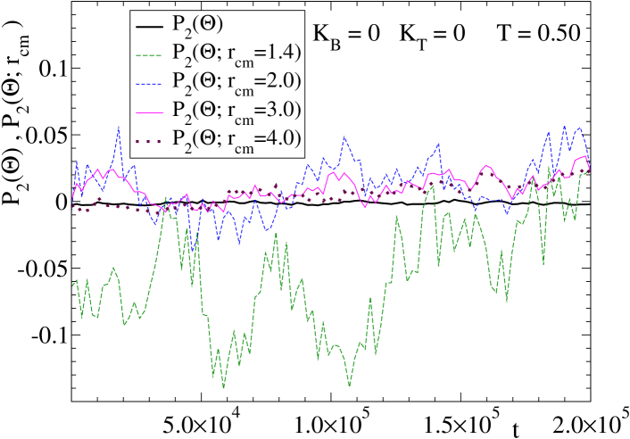
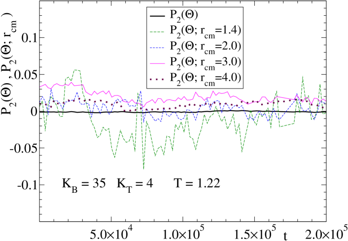
Simulation results presented in this work correspond to isotropic phases. We do not observe signatures of global orientational order induced by chain stiffness for the investigated state points. Thus, by measuring the quantity $P_{2}(\Theta)=(3\langle\cos^{2}\Theta\rangle-1)/2$, where $\Theta$ is the angle between the end-to-end vectors of two chains, and averaging it over all pairs of distinct chains, we obtain in all cases values $|P_{2}(\Theta)|<3\times 10^{-3}$. This is illustrated in Fig. 1, which shows the time evolution of $P_{2}(\Theta)$ along a typical simulation window, both for fully-flexible chains, $(K_{\rm B}$,$K_{\rm T})=$ (0,0), and for representative stiff chains, $(K_{\rm B}$,$K_{\rm T})=$ (35,4).

Local orientational order is also negligible. This is evidenced by computing a similar correlator $P_{2}(\Theta;r_{\rm cm})$. In this case the average is performed only over pairs of distinct chains for which the distance between their respective centers-of-mass is less than $r_{\rm cm}$. Fig. 1 displays, for the former cases of fully-flexible and stiff chains, data of $P_{2}(\Theta;r_{\rm cm})$ for several values of $r_{\rm cm}$. Negligible values of $P_{2}(\Theta;r_{\rm cm})$ are obtained for $r_{\rm cm}\geq 2.0$. Thus, the time average over the simulation time window, $t_{\rm sim}$, provides values $|\langle P_{2}(\Theta;r_{\rm cm}\geq 2.0)\rangle_{\rm t_{\rm sim}}|<0.02$. By comparing both panels we conclude that chain stiffness does not induce a significant increase, if any, of local orientational order. Weak local orientational order $|\langle P_{2}(\Theta;r_{\rm cm})\rangle_{\rm t_{\rm sim}}|\lesssim 0.1$ is observed only for very small interchain distances (see data for $P_{2}(\Theta;r_{\rm cm}=1.4)$). Again, the introduction of chain stiffness does not induce clear changes in the orientational order at this length scale. Note that for small $r_{\rm cm}$ differences in the represented data for different barrier strength may even be statistical artifacts, arising from the small number of neighboring chains within such distances and the limitted time of observation (see the amplitude of the fluctuations in data of Fig. 1).

Figure 1: Time evolution of the global and local orientational parameter (see text) for fully-flexible (top) and stiff chains with $(K_{\rm B}$,$K_{\rm T})=(35,4)$ (bottom), for two selected low temperatures.

b)Static structure factors and chain form factors

Now we present results for static structure factors and chain form factors, both for fully-flexible chains and for a representative case of stiff chains. Let us consider an isotropic homogeneous system of volume $V$ containing $n$ identical chains of $N$ monomers. The densities of chains and monomers are respectively denoted by $\rho_{c}=n/V$ and $\rho=nN/V$. Let us denote the location of a monomer along its chain by the index $1\leq a\leq N$. The site-site static structure factor for monomers of indices $a$ and $b$ is defined as:

$$S_{ab}(q)=\frac{1}{n}\langle\rho_{a}({\bf-q},0)\rho_{b}({\bf q},0)\rangle.$$ (5)

Brackets denote ensemble average. The monomer density distribution for wave vector ${\bf q}$ is given by

$$\rho_{a}({\bf q})=\sum_{j=1}^{n}\exp[i{\bf q}\cdot{\bf r}_{j}^{a}].$$ (6)

In this expresion ${\bf r}_{j}^{a}$ is the position vector of the $a$th monomer in the $j$th chain ($1\leq j\leq n$). The quantity $S_{ab}(q)$ can be splitted into intrachain and interchain $a$-$b$ correlations:

$$S_{ab}(q)=\omega_{ab}(q)+\rho_{c}h_{ab}(q),$$ (7)

or in matrix form, ${\bf S}(q)={\bf w}(q)+\rho_{c}{\bf h}(q)$. In Eq. (7) $\omega_{ab}(q)$ and $h_{ab}(q)$ respectively denote the intrachain and interchain correlations between monomers of type $a$ and $b$. By averaging over all the possible pairs $(a,b)$ we obtain the static correlators $S(q)$, $\omega(q)$ and $h(q)$, which are related through:

$$S(q)=\omega(q)+\rho h(q).$$ (8)

In this expression $S(q)$ is the total static structure factor, which equivalently can be obtained as $S(q)=(nN)^{-1}\langle\rho(-q,0)\rho(q,0)\rangle$, where $\rho(q)=\sum_{a=1}^{N}\rho_{a}(q)$ is the total monomer density distribution. In Eq. (8) the chain form factor, $\omega(q)$, accounts for all the static intrachain correlations, while $h(q)$ accounts for all the static interchain correlations.

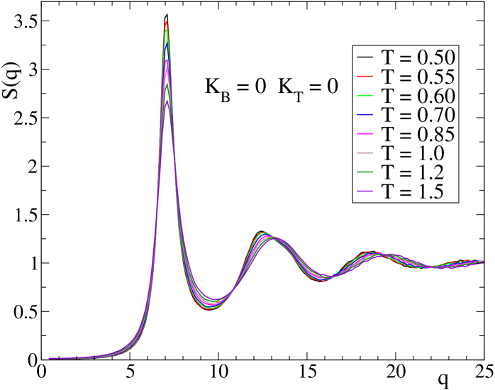
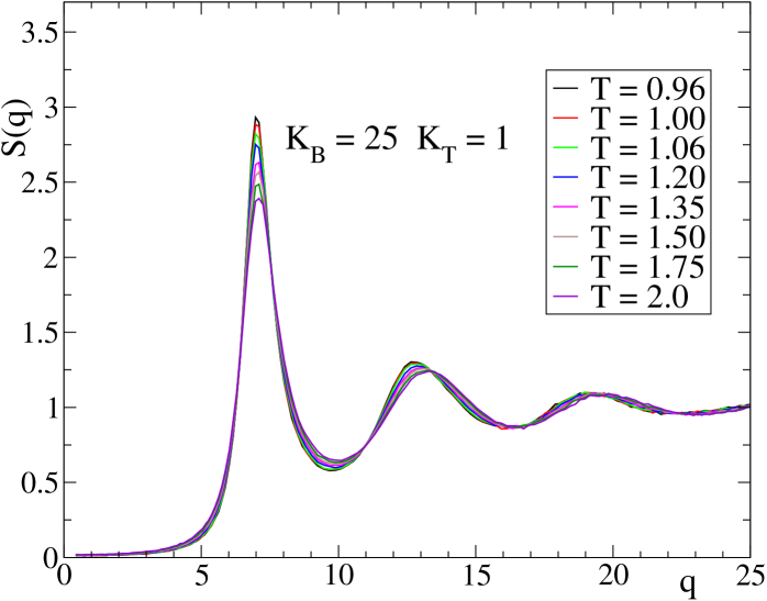
Fig. 2 (top panel) shows simulation results for $S(q)$ as a function of temperature for fully-flexible chains, $(K_{\rm B},K_{\rm T})=(0,0)$. Data for representative stiff chains, $(K_{\rm B},K_{\rm T})=(25,1)$, are shown in the bottom panel. In both cases, no signature of crystallization is present. Indeed no sharp Bragg peaks are observed. In both cases $S(q)$ shows a maximum at $q_{\rm max}\approx 7.0$. Since $S(q_{\rm max})$ comes from the packing in the first shell around a monomer, the latter corresponds to a typical distance $2\pi/7.0\approx 0.90$ in the real space between neighboring monomers. On cooling, the peak at $q_{\rm max}\approx 7.0$ increases in intensity, which is a signature of increasing short-range order.

Figure 2: Temperature dependence of the static structure factor $S(q)$ for fully-flexible chains (top panel) and for chains with barrier strength $(K_{\rm B},K_{\rm T})=(25,1)$ (bottom panel).

In Fig. 3 we show, for the former values of $(K_{\rm B},K_{\rm T})$, the corresponding results for the form factors $\omega(q)$. We note that in the case of fully-flexible chains the form factor is nearly independent on temperature. The form factor for stiff chains exhibits a certain $T$-dependence, which is however rather weak in comparison with that of $S(q)$. The $T$-dependence of $\omega(q)$ becomes more clear at low $q$-values. The way the form factor behaves on lowering the temperature is directly connected with the values of the mean chain end-to-end radius $R_{\rm ee}$. Thus, by decreasing temperature from $T=2.0$ to $T=0.96$, the computed $R_{\rm ee}$ increases from 4.8 to 5.5 for the selected stiff chains. This leads, for lower $T$, to a stronger decay in $\omega(q)$ at low-$q$. On the other hand, the value $R_{\rm ee}=3.6$ for the fully-flexible chains is almost $T$-independent, leading to a negligible $T$-dependence of $\omega(q)$.

Figure 3: Temperature dependence of the form factor $\omega(q)$ for fully-flexible chains (lines) and for chains with barrier strength $(K_{\rm B},K_{\rm T})=(25,1)$ (symbols). For clarity, the inset shows results in the range of low-$q$. Different colors correspond to different temperatures, following the legends of Fig. 2.

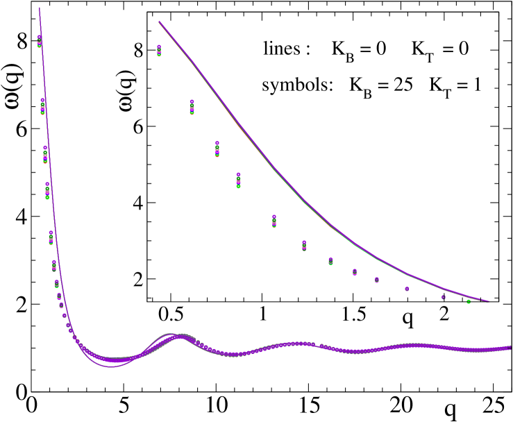
c)Test of the PRISM approximations

The MCT for polymer melts developed by Chong and co-workers chongprl ; chongpre invokes several approximations of the PRISM theory curro . In this subsection we summarize such approximations and test their validity for all the investigated range of barrier strength. The site-site direct correlation function, $c_{ab}(q)$, is introduced via the generalized Ornstein-Zernike relation for polyatomic molecules, or ‘reference interaction site model’ (RISM) rism ,

$$h_{ab}(q)=\sum_{x,y=1}^{N}\omega_{ax}(q)c_{xy}(q)[\omega_{yb}(q)+\rho_{c}h_{yb}(q)],$$ (9)

in which intramolecular contributions are accounted by the form factor terms $\omega_{ab}(q)$. By inserting (7) in Eq. (9), $c_{ab}(q)$ is related to $S_{\rm ab}(q)$ and $\omega_{ab}(q)$ as:

$$\rho_{\rm c}c_{ab}(q)=\omega_{ab}^{-1}(q)-S_{ab}^{-1}(q).$$ (10)

Here $\omega_{ab}^{-1}(q)$ and $S_{ab}^{-1}(q)$ are the elements of, respectively, the matrices ${\bf w}^{-1}(q)$ and ${\bf S}^{-1}(q)$, which are defined as the inverses of ${\bf w}(q)$ and ${\bf S}(q)$.

In the equivalent-site approximation (which is exact for polymer rings) of the PRISM, chain end effects are neglected and all sites are treated equivalently for interchain correlations. Thus, $c_{ab}$ is replaced by the average over all $(a,b)$-pairs:

$$c_{ab}(q)\approx c(q).$$ (11)

By introducing this approximation in Eq. (9) and averaging over all $(a,b)$-pairs we find $h(q)=\omega(q)c(q)[\omega(q)+\rho h(q)]$. By introducing Eq. (8) in the latter expression we arrive to the scalar equation

$$\rho c(q)=1/\omega(q)-1/S(q),$$ (12)

also known as PRISM equation.

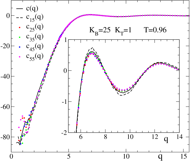
In Figs. 4 and 5 we test the validity of the equivalent-site approximation $c_{ab}(q)\approx c(q)$. We calculate $c_{ab}(q)$ and $c(q)$ respectively through Eqs. (10) and (12), by using the quantities $\omega_{ab}^{-1}(q)$, $S_{ab}^{-1}(q)$, $\omega(q)$, and $S(q)$ as computed from the simulations. Fig. 4 shows results for the fully-flexible case. Data for the case $(K_{\rm B},K_{\rm T})=(25,1)$ are displayed in Fig. 5. Both data sets correspond to the respective lowest investigated temperatures. We use a representation analogous to that of Ref. aichelepre . Thus, top and bottom panels in both figures show the comparison of the averaged $c(q)$ with respectively the matrix elements $c_{aa}(q)$ and $c_{a5}(q)$. The data of Fig. 4 are consistent with results of Ref. aichelepre for a similar fully-flexible bead-spring model. Data in Fig. 5 constitute new results for the case of implemented intramolecular barriers. By looking at both figures we conclude that the quality of the equivalent-site approximation is not altered by the introduction of strong intramolecular barriers. Data in Fig. 5 display the same trends as in the fully-flexible case. Thus, $c_{ab}(q)\approx c(q)$ is an excellent approximation except for correlations involving chain end monomers $a=1$ (and $a=N$ by symmetry). The latter show deviations from $c(q)$ which are moderate around $q_{\rm max}$, this $q$-range being the dominating one in the MCT kernel.

Figure 4: Test of the equivalent site approximation, Eq. (11), for fully-flexible chains at $T=0.50$. Top and bottom panels compare $c(q)$ with respectively matrix elements $c_{aa}(q)$ and $c_{a5}(q)$. The insets enhance the region around the wave vector $q_{\rm max}$ for the maximum of the static structure factor $S(q)$.

Figure 5: Test of the equivalent site approximation, Eq. (11), for stiff chains with $(K_{\rm B},K_{\rm T})=(25,1)$, at $T=0.96$. Top and bottom panels compare $c(q)$ with respectively matrix elements $c_{aa}(q)$ and $c_{a5}(q)$. The insets enhance the region around the wave vector $q_{\rm max}$ for the maximum of the static structure factor $S(q)$.

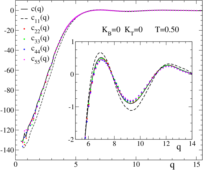
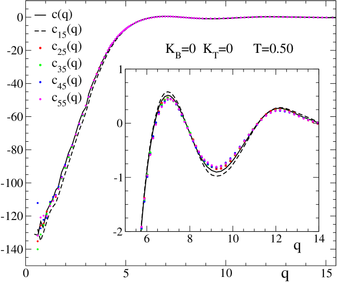
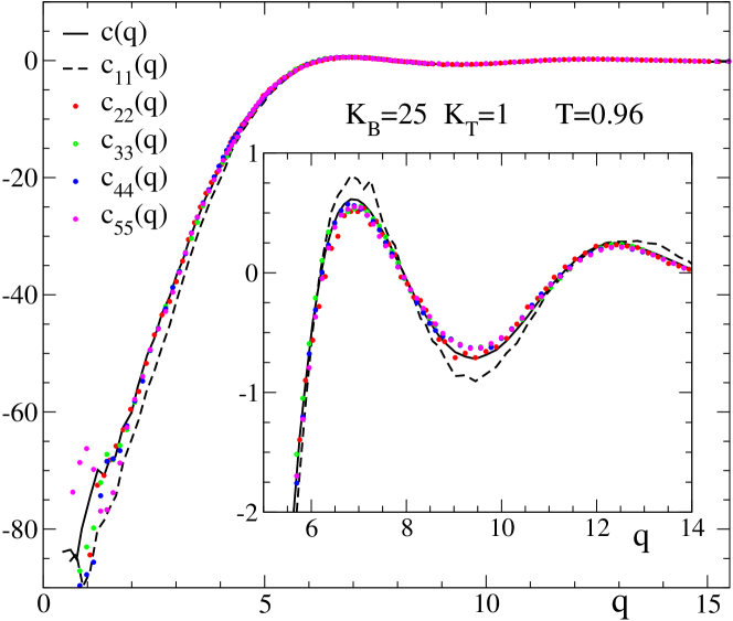
An additional approximation of the PRISM is the ring approximation (which is again exact for polymer rings). First we define the quantities $\tilde{S}_{a}(q)=\sum_{b=1}^{N}S_{ab}(q)$ and $\tilde{S}_{a}^{-1}(q)=\sum_{b=1}^{N}S_{ab}^{-1}(q)$. By exploiting the fact that for a ring polymer $\tilde{S}_{a}(q)$ is $a$-independent, i.e., $\tilde{S}_{a}(q)\approx N^{-1}\sum_{a=1}^{N}\tilde{S}_{a}(q)$, we find

$$\tilde{S}_{a}(q)\approx S(q).$$ (13)

From the definition of $S_{ab}^{-1}(q)$ and $\tilde{S}_{b}(q)$ the relation $\sum_{b=1}^{N}S_{ab}^{-1}(q)\tilde{S}_{b}(q)=1$ is exact. By introducing the ring approximation $\tilde{S}_{b}(q)\approx S(q)$ the former relation is transformed into:

$$\frac{1}{\tilde{S}_{a}^{-1}(q)}\approx S(q).$$ (14)

Fig. 6 shows a test of the ring approximation of Eqs. (13) (main panels) and (14) (insets). This is done both for fully-flexible chains (top panel) and for stiff chains with $(K_{\rm B},K_{\rm T})=(25,1)$ (bottom panel). The comparison between $S(q)$, $\tilde{S}_{a}(q)$ and $1/\tilde{S}_{a}^{-1}(q)$ as computed from simulations is in general excellent, with the same quality for fully-flexible and stiff chains. Only for the end monomers $a=1$ (and $a=N$ by symmetry) significant differences between $S(q)$ and $1/\tilde{S}_{a}^{-1}(q)$ are observed around the wave vector $q_{\rm max}$.

Figure 6: Test of the ring approximation, Eqs. (13,14). Top panel: fully-flexible case at $T=0.50$. Bottom panel: barrier strength $(K_{\rm B},K_{\rm T})=(25,1)$, at $T=0.96$. Main panels and insets compare $S(q)$ (symbols) with respectively $\tilde{S}_{a}(q)$ and 1/$\tilde{S}_{a}^{-1}(q)$, for the sites $a=$ 1,2 and 5 (lines).

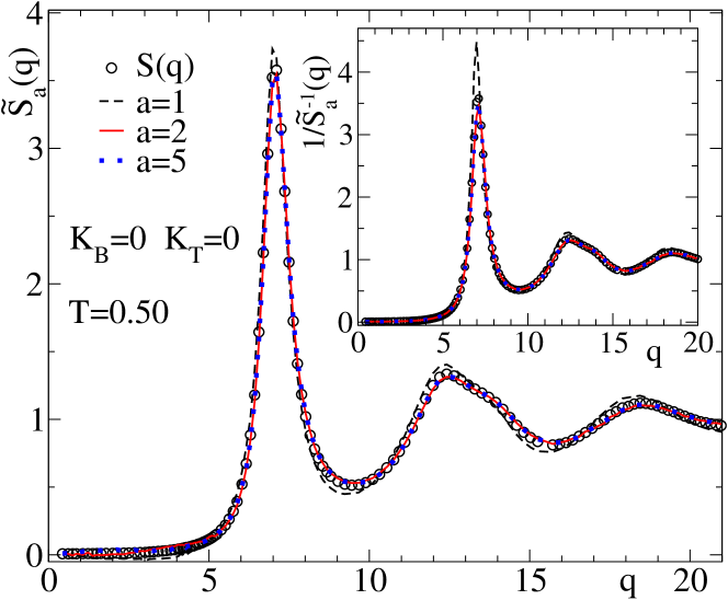
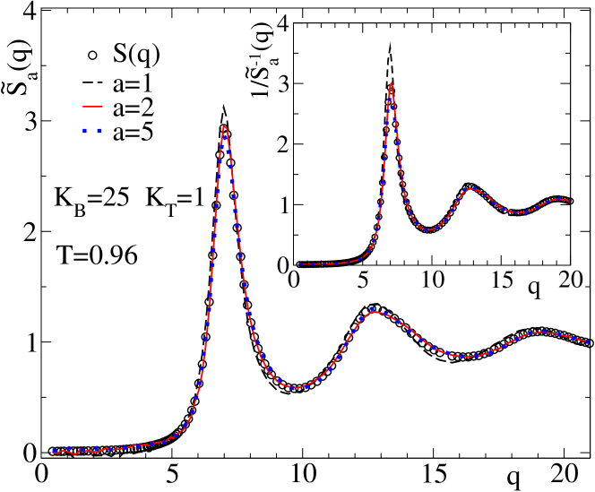
With all these results we conclude that the approximations assumed by the PRISM theory and introduced in the MCT equations for polymer melts (see below) are fulfilled, with the same quality for all the investigated range of barrier strength.

IV. DYNAMIC PROPERTIES

In this section we show some phenomenological dynamic features induced by the introduction of intramolecular barriers in our model. Panels in Fig. 7 show the $T$-dependence of the monomer mean squared displacement (MSD) for fully-flexible and representative stiff chains with $(K_{\rm B},K_{\rm T})=(25,1)$. We observe similar features in both cases, but also some differences. After the initial ballistic regime, a plateau extends over longer times with decreasing temperature. This plateau corresponds to the caging regime — i.e., the temporary trapping of each monomer in the shell of neighboring monomers around it — which is usually observed when approaching a liquid-glass transition. At longer times, leaving the plateau, a crossover to a Rouse-like sublinear regime $\langle(\Delta r)^{2}\rangle\propto t^{0.65}$ bennemann ; aichele is observed for the fully-flexible case. The final crossover to linear diffusion $\langle(\Delta r)^{2}\rangle\propto t$ is reached at long times only for the highest investigated temperatures. However, for the case of stiff chains it is difficult to discriminate power-law behavior over significant time windows. Apparently, the linear diffusive regime is not reached within the simulation time window.

Figure 7: Temperature dependence of the monomer mean squared displacement for fully-flexible (top) and stiff chains with $(K_{\rm B},K_{\rm T})=(25,1)$ (bottom). The solid and dashed lines indicate respectively sublinear ($\sim t^{0.65}$) and linear behavior.

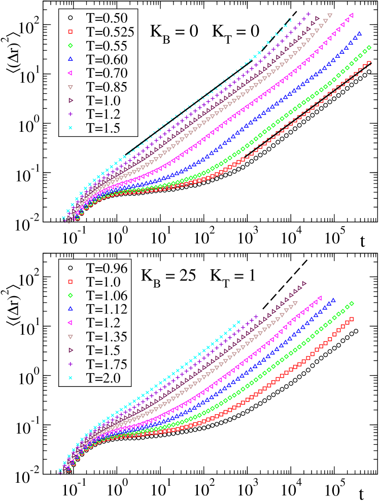
Fig. 8 shows the monomer MSD, for fixed values of density $\rho=1.0$ and temperature $T=1.5$, as a function of the barrier strength. Consistently with results in Ref. bulacu2 , we observe that increasing the strenght of the internal barriers at fixed $\rho$ and $T$ leads to slower dynamics.

Figure 8: Monomer mean squared displacement, for several values of the barrier strength, at fixed density $\rho=1.0$ and temperature $T=1.5$.

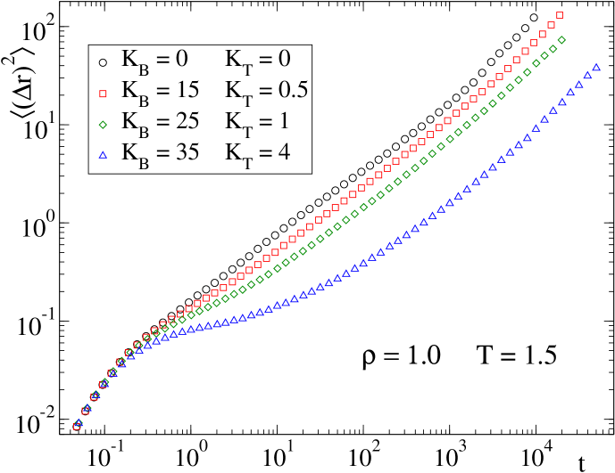
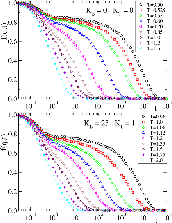
Fig. 9 shows simulation results at several temperatures, both for fully-flexible and stiff chains, for the normalized density-density correlator $f(q,t)$. The latter is defined as $f(q,t)=\langle\rho(-q,0)\rho(q,t)\rangle/\langle\rho(-q,0)\rho(q,0)\rangle$. In both cases the correlator is evaluated at the maximum, $q_{\rm max}\approx 7$, of the static structure factor $S(q)$. As in the case of the MSD, both the fully-flexible and stiff cases exhibit the standard behavior in the proximity of a glass transition bennemann ; aichele . After the initial transient regime, $f(q,t)$ shows a first decay to a plateau connected with the caging regime. On lowering the temperature this plateau extends over longer time intervals. At long times, a second decay is observed from the plateau to zero. This second decay corresponds to the structural $\alpha$-relaxation.

Figure 9: Temperature dependence of $f(q,t)$ for fully-flexible (top) and stiff chains with $(K_{\rm B},K_{\rm T})=(25,1)$ (bottom). The wave vector is $q_{\rm max}\approx 7$, in both cases corresponding to the maximum of the static structure factor $S(q)$.

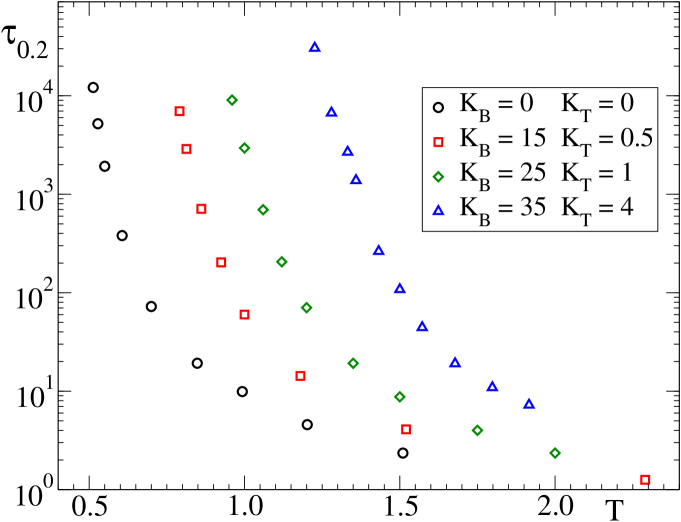
Let us define the relaxation time as a time scale probing the $\alpha$-structural relaxation. This can be done by introducing the time $\tau_{x}$ for which the correlator for $q_{\rm max}$ takes the value $f(q_{\rm max},\tau_{x})=x$, provided $x$ is small in comparison with the plateau height. Here we use $x=0.2$. Fig. 10 shows $\tau_{0.2}$ as a funcion of $T$, for different values of the bending and torsional constants. As observed in the analysis of the mean squared displacements, increasing the chain stiffness slows down the dynamics. At fixed temperature, the relaxation time for the stiffest investigated chains increases up to three decades with respect to the fully-flexible case.

In this section we have demonstrated a main dynamic feature: the slowing down of the dynamics, at fixed density and temperature, by progressively increasing the strength of the intramolecular barriers. This feature strongly suggests that intramolecular barriers constitute and additional mechanism for dynamic arrest, coexisting with the general packing effects induced by density and temperature. In the following we summarize the main predictions of the Mode Coupling Theory and discuss simulation dynamic features within this theoretical framework.

Figure 10: Temperature dependence of the relaxation times $\tau_{0.2}$ for several values of the barrier strength.

V. MODE COUPLING THEORY: SUMMARY

In this section we briefly summarize universal dynamic scaling laws concerning the MCT liquid-glass dynamics, and test them in the simulated polymer melt for all the investigated range of barrier strength. Extensive reviews on MCT can be found, e.g., in Refs. mctrev1 ; mctrev2 ; gotzebook ; reichman ; das ; gotzenewbook ; franosch ; fuchspre . Though initially derived for simple hard-sphere systems, these predictions follow as consequences of the mathematical structure of the MCT equations. More specifically, they are associated to the bilinear dependence of the memory kernel on the density correlators (see below). Thus, MCT predicts the same dynamic scaling laws of the monoatomic case if such a mathematical structure is retained in systems of polyatomic molecules. This is indeed the case of the MCT for polymer melts developed by Chong and co-workers chongprl ; chongpre (see below). Therefore, the phenomenological analysis of our simulation results in terms of MCT dynamic scaling laws is justified within the theory.

By starting from the fundamental Liouville equation of motion and using the Mori-Zwanzig projection operator formalism one arrives to an integro-differential equation for the normalized density-density correlator:

$$\ddot{f}(q,t)+\frac{q^{2}k_{B}T}{mS(q)}f(q,t)\hskip 56.9055pt$$

$$+\frac{q^{2}k_{B}T}{mS(q)}\int^{t}_{0}dt^{\prime}m(q,t-t^{\prime})\dot{f}(q,t^{\prime})=0.$$ (15)

This equation is obtained by using projectors over the subspace spanned by the densities and the longitudinal currents. The memory kernel $m(q,t-t^{\prime})\propto\langle R_{q}(0)R_{q}(t-t^{\prime})\rangle$, where the quantities $R_{q}$ are, within the Mori-Zwanzig formalism, the associated fluctuating forces. Since the kernel cannot be exactly expressed in terms of $f(q,t)$ and/or its time derivatives, Eq. (15) is not solvable. MCT introduces several approximations for the memory kernel, in order to provide a closed solvable form of Eq. (15). These approximations are:

i) It is assumed that the long-time, slow dynamic regime of any observable coupled to density fluctuations can be expressed as a linear combination of ‘mode pairs’, $\rho_{{\bf k}}\rho_{{\bf q-k}}$. Since the exact expression of the correlator of the fluctuating forces contains a slow contribution which is a linear combination of mode pairs (see e.g., Ref. reichman for details), the former assumption is equivalent to neglecting the fast contribution of the fluctuating forces. In other words, it is equivalent to assuming a large separation between the time scales of the former contributions.

ii) Convolution approximation: three-point static correlations are approximated as products of static structure factors,

$$\langle\rho_{-{\bf q}}(0)\rho_{{\bf k}}(0)\rho_{{\bf q}-{\bf k}}(0)\rangle\approx nNS(q)S(k)S(|{\bf q}-{\bf k}|).$$ (16)

iii) Kawasaki approximation: dynamic four-point correlations are factorized in terms of products of dynamic two-point correlations,

$$\langle\rho_{{\bf k}-{\bf q}}(0)\rho_{-{\bf q}}(0)\rho^{\cal{Q}}_{{\bf q}-{\bf k}}(t)\rho^{\cal{Q}}_{{\bf q}}(t)\rangle\approx\hskip 28.45274pt$$

$$F(q,t)F(|{\bf q}-{\bf k}|,t),$$ (17)

where the superscript $\cal{Q}$ denotes evolution with projected dynamics (see e.g., Ref. reichman for details), and $F(q,t)=\langle\rho(-q,0)\rho(q,t)\rangle$ are just the unnormalized density-density correlators.

By making use of these three approximations, the memory kernel $m(q,t)$ becomes a bilinear form in $f(q,t)$,

$$m(q,t)=\int\frac{d^{3}{\bf k}}{(2\pi)^{3}}{\cal V}({\bf q}-{\bf k},{\bf k})f(k,t)f(|{\bf q}-{\bf k}|,t),$$ (18)

where the vertex ${\cal V}({\bf q}-{\bf k},{\bf k})$ is given by:

$${\cal V}({\bf q}-{\bf k},{\bf k})=\frac{\rho}{2q^{4}}S(q)S(k)S(|{\bf q}-{\bf k}|)\times$$

$$\left[{\bf q}\cdot{\bf k}c({\bf k})+{\bf q}\cdot({\bf q}-{\bf k})c(|{\bf q}-{\bf k}|)\right]^{2}.$$ (19)

In a monoatomic fluid the direct correlation function $c(q)$ is related to the static structure factor via the exact Ornstein-Zernike relation hansen $\rho c(q)=1-S^{-1}(q)$. With all this, Eq. (15) has been reduced to a closed set of coupled equations which can be solved self-consistently, provided $S(q)$ and $c(q)$ are known (the latter are external inputs in the MCT equations).

For the case of systems with molecular architecture, Chong and Hirata have obtained chonghirata , by using projectors over site-densities and site-currents, generalized MCT equations of motion for site-site correlators $F_{ab}(q,t)$. The latter are defined as $F_{ab}(q,t)=n^{-1}\langle\rho_{a}(-q,0)\rho_{b}(q,t)\rangle$. Note that $F_{ab}(q,0)=S_{ab}(q)$. The corresponding MCT equations of motion are

$$\ddot{F}_{ab}(q,t)+\frac{q^{2}k_{\rm B}T}{m}\sum_{x=1}^{N}S_{ax}^{-1}(q)F_{xb}(q,t)$$

$$+\sum_{x=1}^{N}\int_{0}^{t}dt^{\prime}M_{ax}(q,t-t^{\prime})\dot{F}_{xb}(q,t^{\prime})=0,$$ (20)

where the memory kernel is now given by

$$M_{ab}(q,t)=\frac{\rho_{c}k_{\rm B}T}{mq^{2}}\sum_{x,y=1}^{N}\int\frac{d^{3}{\bf k}}{(2\pi)^{3}}\times$$

$$\{({{\bf q}}\cdot{\bf k})^{2}c_{ax}(k)c_{by}(k)F_{xy}(k,t)F_{ab}(p,t)$$

$$+({{\bf q}}\cdot{\bf k})({{\bf q}}\cdot{\bf p})c_{ax}(k)c_{by}(p)F_{xb}(k,t)F_{ay}(p,t)\},$$ (21)

with ${\bf p}={\bf q}-{\bf k}$. By comparing Eqs. (20,21) with Eqs. (15,18,19) we note that the general mathematical structure of the kernel (bilinear in site-site correlators), and of the MCT equations of motion is retained.

Except for very small values of $N$, numerical solution of the MCT equations for site-site correlators is extremely expensive, and further simplifications are needed in order to obtain a tractable set of equations. For the case of simple bead-spring chains, Chong and co-workers have reduced chongprl ; chongpre Eqs. (20,21) to a scalar form for $f(q,t)$. This is achieved by introducing in Eqs. (20,21) the equivalent site, Eq. (11), and ring, Eqs. (13,14), approximations of the PRISM theory. The so-obtained scalar MCT equations of motion, memory kernel and vertex for polymer chains are formally identical to Eqs. (15,18,19). The polymer character of the system only enters implicitly through the PRISM relation $\rho c(q)=1/\omega(q)-1/S(q)$, which differs from the Ornstein-Zernike equation, $\rho c(q)=1-S^{-1}(q)$, for monoatomic systems. With this, general MCT predictions which originate from the mathematical structure of Eqs. (15,18,19) will be, due to the mentioned formal equivalence, analogous both for monoatomic systems and for polymer chains. Now we summarize such general predictions.

In MCT, nonergodic arrested states (glasses) are defined as those for which density correlators do not exhibit full relaxation. More specifically, if we introduce the nonergodicity parameters, defined as $f_{q}=\lim_{t\rightarrow\infty}f(q,t)$, MCT discriminates between fluid states ($f_{q}=0$) and glassy states ($f_{q}>0$). At the MCT critical temperature $T_{\rm c}$, the nonergodicity parameters jump from zero to nonzero values hopping . In the following we use the notation $f^{\rm c}_{q}$ for referring to the critical nonergodicity parameters, i.e., the values of $f_{q}$ at $T=T_{\rm c}$.

By Laplace transform ($t\rightarrow z$) of Eqs. (15,18) and taking the limit $z\rightarrow 0$, one finds a coupled set of equations for the nonergodicity parameters:

$$\frac{f_{q}}{1-f_{q}}={\cal F}_{q}(\{f\})=\int\frac{d^{3}{\bf k}}{(2\pi)^{3}}{\cal V}({\bf q}-{\bf k},{\bf k})f_{|{\bf q}-{\bf k}|}f_{k},$$ (22)

where ${\cal F}_{q}(\{f\})$ denotes a functional, whose explict expression is given in the right-hand side of the equation. Note that Eq. (22) always has the trivial solution ${f_{q}=0}$. Thus, glassy states take place when solutions $f_{q}>0$ also exist.

Given a tagged chain (labeled s), the density distribution for the $a$th monomer of the tagged chain is defined as $\rho^{\rm s}_{a}(q)=\exp[i{\bf q}\cdot{\bf r}^{a}_{\rm s}]$. The site-site intrachain correlator is defined as $F^{\rm s}_{ab}(q,t)=\langle\rho^{\rm s}_{a}(-q,0)\rho^{\rm s}_{b}(q,t)\rangle$. Note that $F^{\rm s}_{ab}(q,0)=\omega_{ab}(q)$. For the derivation of the MCT equations for $F_{ab}^{\rm s}(q,t)$ we refer to chongpre . In this case the reduction to a scalar form is not possible. The corresponding nonergodicity parameters $f_{ab}^{s}(q)=\lim_{t\rightarrow\infty}F_{ab}^{s}(q,t)$ are obtained by solving the $N\times N$-matrix equation chongdum

$$f_{ab}^{s}(q)=\sum_{x,y=1}^{N}{\cal F}_{ax}^{s}(q)[{\bf I}+{\boldmath\cal{F}}_{q}^{s}]_{xy}^{-1}\omega_{yb}(q),$$ (23)

with ${\bf I}$ the identity matrix. The corresponding functional ${\cal F}_{ab}^{s}(q)$ is given by

$${\cal F}_{ab}^{s}(q)=\sum_{x=1}^{N}\omega_{ax}(q)\int\frac{d^{3}{\bf k}}{(2\pi)^{3}}\times$$

$${\cal V}^{s}({\bf q}-{\bf k},{\bf k})f_{xb}^{s}(k)f_{|{\bf q}-{\bf k}|},$$ (24)

with the vertex

$${\cal V}^{s}({\bf q}-{\bf k},{\bf k})=\frac{\rho}{q^{4}}S(|{\bf q}-{\bf k}|)[{\bf q}\cdot({\bf q}-{\bf k})]^{2}c^{2}(|{\bf q}-{\bf k}|).$$ (25)

The normalized self-correlator, usually introduced as $f^{\rm s}(q,t)=(nN)^{-1}\sum^{n}_{j=1}\sum^{N}_{a=1}\langle\exp[i{\bf q}\cdot({\bf r}^{a}_{j}(t)-{\bf r}^{a}_{j}(0))]\rangle$, can be equivalently obtained as $f^{\rm s}(q,t)=N^{-1}\sum_{a=1}^{N}F_{aa}^{s}(q,t)$. Likewise, the corresponding nonergodicity parameters, defined as the long-time limit of $f^{\rm s}(q,t)$, can be obtained as $f_{q}^{\rm s}=N^{-1}\sum_{a=1}^{N}f_{aa}^{s}(q)$. Thus, the solution of Eq. (23) also provides trivially the nonergodicity parameters for the self-correlator.

The separation parameter, $\epsilon=(T-T_{\rm c})/T_{\rm c}$, is introduced to quantify the relative distance to the critical temperature $T_{\rm c}$. We are interested in the behavior of $f(q,t)$ in the ergodic fluid by approaching $T_{c}$ from above. Thus we express the long-time behavior of the density-density correlators as:

$$f(q,t)=f^{\rm c}_{q}+g_{q}(t),$$ (26)

where $g_{q}(t)$ quantifies (small) deviations around $f^{\rm c}_{q}$ for $|\epsilon|\rightarrow 0$. By introducing Eq. (26) in Eqs. (15,18), expanding the functional ${\cal F}_{q}$ of Eq. (22) in a power series of $|\epsilon|$, comparing the so-obtained resulting expressions and retaining the lower-order terms (see, e.g., Ref. franosch for a detailed exposition), one finds that $g_{q}(t)=h_{q}G(t)$, where $h_{q}$ only depends on $q$, and $G(t)$ is a $q$-independent term which contains the full time dependence of the deviations of $f(q,t)$ around $f^{\rm c}_{q}$. Thus, we rewrite Eq. (26) as:

$$f(q,t)=f^{\rm c}_{q}+h_{q}G(t).$$ (27)

This expression is known as the first universality of the MCT or factorization theorem. It predicts a scaling function $G(t)$ (known as the $\beta$-correlator) that is common for all the density correlators (since it is $q$-independent). Following the procedure mentioned in the previous paragraph franosch , the function $G(t)$ is found to obey the equation:

$$\sigma-z^{2}\tilde{G}^{2}(z)=\lambda zL[G^{2}(t)],$$ (28)

where $\tilde{G}(z)$ and $L[G^{2}(t)]$ are the Laplace transform of respectively $G(t)$ and $G^{2}(t)$. In this equation $\sigma=c|\epsilon|$, with $c$ a constant (see franosch for its explicit expression), and $\lambda$ is another constant given by

$$\lambda=\sum_{qk}e^{\rm T}_{q}C^{\rm c}(q,k,|{\bf q}-{\bf k}|)e_{k}e_{|{\bf q}-{\bf k}|}.$$ (29)

The quantities $e_{q}$ and $e^{\rm T}_{q}$ are respectively the eigenvectors of the so-called stability matrix ${\bf C}^{\rm c}$ (see below) and its traspose, with the normalization conditions $\sum_{q}e^{\rm T}_{q}e_{q}=1$ and $\sum_{q}e^{\rm T}_{q}(1-f^{\rm c}_{q})e^{2}_{q}=1$. The elements of the stability matrix are given by

$$C^{\rm c}(q,k)=(1-f^{\rm c}_{k})^{2}\left(\frac{\partial{\cal F}_{q}}{\partial f_{k}}\right)_{\{f=f^{\rm c}\}}.$$ (30)

The terms $C^{\rm c}(q,k,|{\bf q}-{\bf k}|)$ in Eq. (29) are given by:

$$C^{\rm c}(q,k,|{\bf q}-{\bf k}|)=\hskip 113.81102pt$$

$$\frac{1}{2}(1-f^{\rm c}_{k})^{2}(1-f^{\rm c}_{|{\bf q}-{\bf k}|})^{2}\left(\frac{\partial^{2}{\cal F}_{q}}{\partial f_{k}\partial f_{|{\bf q}-{\bf k}|}}\right)_{\{f=f^{\rm c}\}}.$$ (31)

Eq. (28) for the $\beta$-correlator does not have an analytical solution. Still, asymptotic expressions can be obtained for different time windows. With this idea in mind the $\beta$-time scale is first defined as

$$\tau_{\beta}=t_{0}|\sigma|^{-1/(2a)}$$ (32)

with $t_{0}$ a microscopic time scale and $a$ an exponent. The $\beta$-correlator is then rewritten as $G(t)=|\sigma|^{1/2}g_{\sigma}(t/\tau_{\beta})$. By introducing this expression in Eq. (28) and taking the limits $t\ll\tau_{\beta}$ and $t\gg\tau_{\beta}$ one finds the asymptotic solutions gotzebook :

$$g_{\sigma}(t/\tau_{\beta})=(t/\tau_{\beta})^{-a}\hskip 28.45274ptt\ll\tau_{\beta},$$ (33)

$$g_{\sigma}(t/\tau_{\beta})=-B(t/\tau_{\beta})^{b}\hskip 28.45274ptt\gg\tau_{\beta},$$ (34)

where $B$ is a constant franosch . The exponents $a$ and $b$ follow the constraint

$$\lambda=\frac{\Gamma^{2}(1-a)}{\Gamma(1-2a)}=\frac{\Gamma^{2}(1+b)}{\Gamma(1+2b)},$$ (35)

where $\Gamma$ denotes the Euler’s Gamma function. According to Eqs. (33,34), one finds the asymptotic expressions for Eq. (27):

$$f(q,t)=f^{\rm c}_{q}+h_{q}(t/t_{0})^{-a}\hskip 28.45274ptt\ll\tau_{\beta},$$ (36)

$$f(q,t)=f^{\rm c}_{q}-h_{q}(t/\tau_{\alpha})^{b}\hskip 28.45274ptt\gg\tau_{\beta}.$$ (37)

The analysis of the long-time decay usually includes higher-order corrections franosch to Eq. (37):

$$f(q,t)=f^{\rm c}_{q}-h_{q}(t/\tau_{\alpha})^{b}+h_{q}^{(2)}(t/\tau_{\alpha})^{2b}+O(t^{3b}).$$ (38)

The latter is also known as the von Schweidler expansion. In these equations $\tau_{\alpha}$ is the $\alpha$-time scale, defined as:

$$\tau_{\alpha}=B^{-1/b}t_{0}|\sigma|^{-\gamma}.$$ (39)

The exponent $\gamma$ follows the constraint:

$$\gamma=\frac{1}{2a}+\frac{1}{2b}.$$ (40)

Another important prediction of the MCT for states approaching $T_{\rm c}$ from above, is the second universality or time-temperature superposition principle (TTSP). This prediction arises as a long-time scaling property of the MCT equations of motion gotzebook . According to the TTSP, the long-time decay of any correlator $f(q,t)$ (i.e. the final part of the $\alpha$-relaxation) is invariant under scaling by the $\alpha$-relaxation time $\tau_{\alpha}$. In other words, for two temperatures $T_{1}$ and $T_{2}$ above $T_{\rm c}$ one finds

$$f(q,t/\tau_{\alpha}(T_{1});T_{1})=f(q,t/\tau_{\alpha}(T_{2});T_{2})=\widetilde{f}(q,\hat{t}),$$ (41)

where $\widetilde{f}(q,\hat{t})$ is a $T$-independent master function of the normalized time $\hat{t}$. While $G(t)$ is common to all correlators, the master function $\widetilde{f}(q,\hat{t})$ associated to the TTSP is different for each correlator $f(q,t)$. The superposition principle implies that the estimated $\alpha$-relaxation time, defined in this work as the time $\tau_{x}$ where $f(q_{\rm max},t)$ takes a value $x$ well below the plateau, is proportional to $\tau_{\alpha}$. Thus, it also follows the asymptotic power law

$$\tau_{x}(T)\propto(T-T_{\rm c})^{-\gamma}.$$ (42)

The $\alpha$-decay from the plateau to zero is often well described by an empirical Kohlrausch-Williams-Watts (KWW) function,

$$f(q,t)=A_{q}\exp[-(t/\tau^{K}_{q})^{\beta_{q}}],$$ (43)

with $A_{q},\beta_{q}<1$. Note that the latter does not come out as an analytical solution of the MCT equations. However in the limit $q\rightarrow\infty$ of the KWW time $\tau^{K}_{q}$, MCT predicts that fuchsjcns

$$\tau^{K}_{q}\propto q^{-1/b}\hskip 28.45274ptq\rightarrow\infty,$$ (44)

where $b$ is the von Schweidler exponent introduced above.

The set of equations exposed in this section constitute a series of universal results which originate from the structure of the MCT equations of motion, Eqs. (15,18,19). As mentioned above, the latter were initially derived for simple hard-sphere systems, but the corresponding ones for polymer melts become formally identical following the derivation by Chong and co-workers chongprl ; chongpre . With this, the scaling laws exposed in this section will also hold in the MCT for polymer melts. Thus, the phenomenological analysis of our simulation data in terms of such scaling laws is justified within the framework of MCT. This analysis is presented in the next section.

VI. MCT ANALYSIS OF SIMULATIONS

In order to test the factorization theorem, Eq. (27), we compute the ratio:

$$R_{q}(t)=\frac{f(q,t)-f(q,t^{\prime})}{f(q,t^{\prime\prime})-f(q,t^{\prime})}=\frac{G(t)-G(t^{\prime})}{G(t^{\prime\prime})-G(t^{\prime})}$$ (45)

where $t^{\prime}$ and $t^{\prime\prime}$ are arbitrary times in the $\beta$-regime. The ratio for the self-correlators, $R^{\rm s}_{q}(t)$, is defined analogously. If the factorization theorem, and then also the right-hand side of Eq. (45), is fulfilled, the ratios $R_{q}(t)$ and $R^{\rm s}_{q}(t)$ do not depend on the specific correlator. Fig. 11 shows $R_{q}(t)$ and $R_{q}^{\rm s}(t)$ over a broad range of wave vectors $2.3\leq q\leq 16.5$. The data correspond to barrier strength $(K_{\rm B},K_{\rm T})=(15,0.5)$ at $T=0.80$. The fixed times $t^{\prime\prime}=0.8$ and $t^{\prime}=100$ roughly correspond to the beginning and the end of the plateau regime. There is an intermediate time window of about two decades where the data for density-density and self-correlators collapse onto a $q$-independent master curve, while they split at both short and late times. Fig. 12 demonstrates that the master curve is, moreover, the same for both density-density and self-correlators. Thus, Figs. 11 and 12 demonstrate the validity of the MCT first universality.

Figure 11: Test of the factorization theorem, Eq. (45), for density-density (top) and self-correlators (bottom) at $T=0.80$ and $(K_{\rm B},K_{\rm T})=(15,0.5)$. The different curves correspond to equispaced wave vectors in the range $2.3\leq q\leq 16.5$. The fixed times are $t^{\prime}=100$ and $t^{\prime\prime}=0.8$.

Figure 12: Common representation of $R_{q}(t)$ (symbols) and $R_{q}^{\rm s}(t)$ (lines), for selected wavevectors (common colors correspond to common $q$-values). As in Fig. 11, data correspond to $T=0.80$ and $(K_{\rm B},K_{\rm T})=(15,0.5)$, and the selected fixed times are $t^{\prime}=100$ and $t^{\prime\prime}=0.8$.

Figure 13: Test of the time-temperature superposition principle, Eq. (41), for the density-density correlators at $q_{\rm max}\approx 7$, for the case $(K_{\rm B},K_{\rm T})=(15,0.5)$.

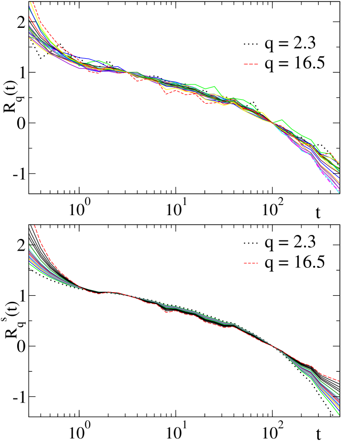
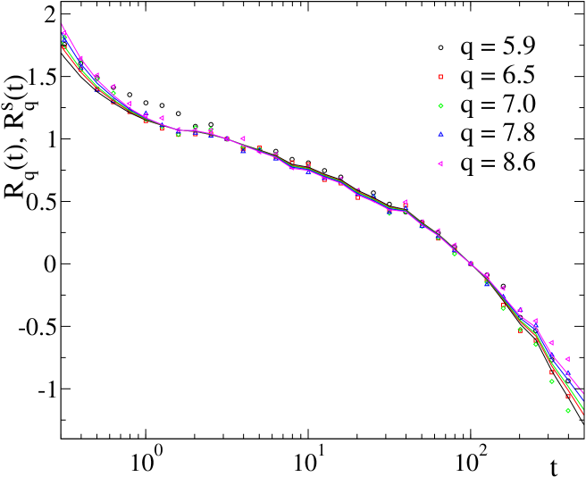
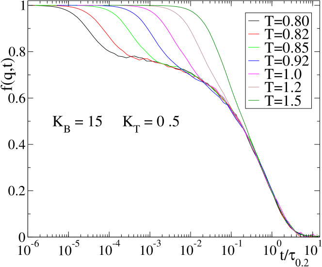
Fig. 13 shows a test of the TTSP, Eq. (41), for the density-density correlator evaluated at $q_{\rm max}$ (maximun of the static structure factor $S(q)$). The data correspond to the case $(K_{\rm B},K_{\rm T})=(15,0.5)$ and cover a broad temperature range $0.80\leq T\leq 1.5$. Data collapse onto a master curve after rescaling the absolute time by the relaxation time $\tau_{0.2}$. Thus, the MCT second universality also holds for chains with strong intramolecular barriers.

Figure 14: Symbols: simulations results for density correlators. Top panel: $f(q,t)$ for $(K_{\rm B},K_{\rm T})=(15,0.5)$, at $T=0.80$. Bottom panel: $f^{\rm s}(q,t)$ for $(K_{\rm B},K_{\rm T})=(35,4)$, at $T=1.33$. Identical symbols in both panels correspond to identical wave vectors $q$ [values are given in panel (a)]. Lines are fits to the von Schweidler expansion, Eq. (38) (up to second-order terms), with $b=0.50$ (top) and 0.37 (bottom).

Solving numerically the MCT equations and determining the dynamic exponents $(a,b,\gamma,\lambda)$ is in general a difficult task. When numerical solutions are not available, nonergodicity parameters, prefactors and exponents in Eqs. (36,38,42,44) can be obtained as fit parameters from simulation or experimental data (see, e.g., Refs. mctrev2 ; aichele ; vanmegen ; koband2 ; baschrev ). Consistency of the analysis requires that dynamic correlators and relaxation times are described by a common set of exponents, all of them related to a single $\lambda$-parameter through Eqs. (35,40).

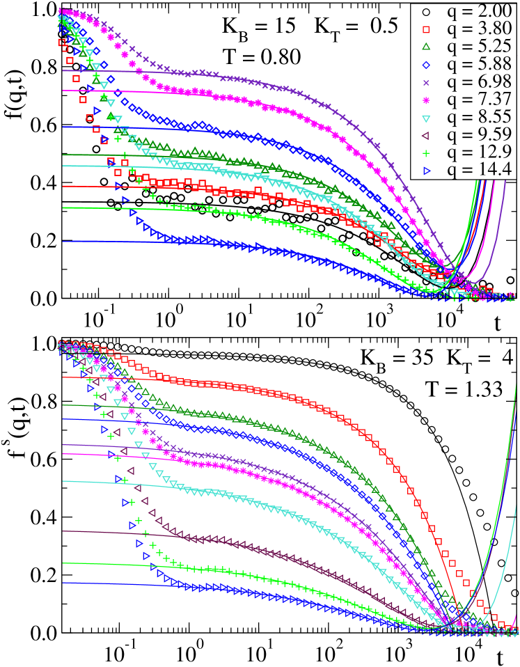
We have performed this consistency test for all the investigated range of barrier strength. The following figures in this section illustrate, for some representative cases, the analysis of simulation data in terms of MCT asymptotic laws. Fig. 14 shows for a broad $q$-range ($2.0\leq q\leq 14.4$), fits to the von Schweidler expansion, Eq. (38) (up to second-order terms). Data correspond to density-density correlators $f(q,t)$ for the state point $(K_{\rm B},K_{\rm T})=(15,0.5)$, $T=0.80$ (labelled S1), and to self-correlators $f^{\rm s}(q,t)$ for $(K_{\rm B},K_{\rm T})=(35,4)$, $T=1.33$ (labelled S2). A good description of the simulation data is achieved, for all the range of $q$-values and over almost four time decades, with a fixed $b$-exponent ($b=0.50$ and 0.37 for respectively S1 and S2).

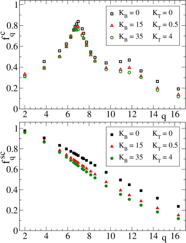
Fig. 15 displays, for the former values of the barrier strength, the $q$-dependence of the so-obtained critical nonergodicity parameters ($f_{q}^{\rm c}$ for $f(q,t)$ and $f_{q}^{\rm sc}$ for $f^{\rm s}(q,t)$). For comparison, we also include the fully-flexible case $(K_{\rm B},K_{\rm T})=(0,0)$. As deduced from the stronger decay of $f_{q}^{\rm c}$ and $f_{q}^{\rm sc}$ for stronger barriers, the introduction of chain stiffness yields a weaker stability of density fluctuations. It also induces a weaker localization for self-motions at fixed density. Thus, by making an approximate fit of $f_{q}^{\rm sc}$ to Gaussian behavior, $f_{q}^{\rm sc}\approx\exp(-q^{2}l_{\rm c}^{2}/6)$, we estimate, at fixed $\rho=1.0$, a localization length $l_{\rm c}=$ 0.19, 0.21, and 0.23 for respectively $(K_{\rm B},K_{\rm T})=$ (0,0), (15,0.5), and (35,4).

Figure 15: Critical nonergodicity parameters, as determined from fits to Eq. (38), for different barrier strength. Top and bottom panels show data for respectively $f_{q}^{\rm c}$ and $f_{q}^{\rm sc}$.

Data of self-correlators from the plateau to the limit of the simulation window have been fitted to KWW functions, Eq. (43) (not shown). Fig. 16 shows the $q$-dependence of the so-obtained KWW relaxation times $\tau_{q}^{\rm K}$ for the former values of the barrier strength, at their respective lowest investigated temperatures. The lines represent tests of the MCT prediction $\tau_{q}^{\rm K}\propto q^{-1/b}$ for large $q$. A good description of the data is obtained with the same $b$-exponents used for the independently obtained von Schweidler fits of Fig. 14.

Figure 16: Symbols: $q$-dependence of KWW relaxation times for different barrier strength. Lines are fits to $\propto q^{-1/b}$ (see text). From top to bottom $b=0.54$, 0.50 and 0.37.

Figure 17: Symbols: $T$-dependence of relaxation times $\tau_{0.2}$ for different barrier strength. Lines are fits to $\propto(T-T_{\rm c})^{-\gamma}$ (see text). From top to bottom $\gamma=2.60$, 2.74 and 3.43.

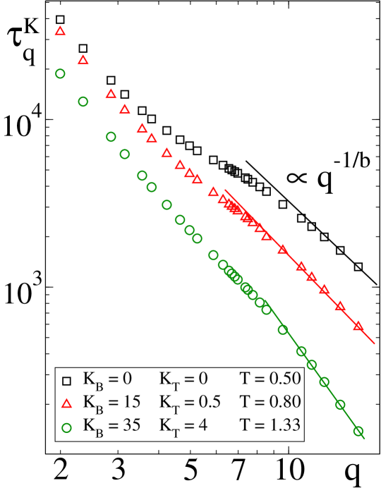
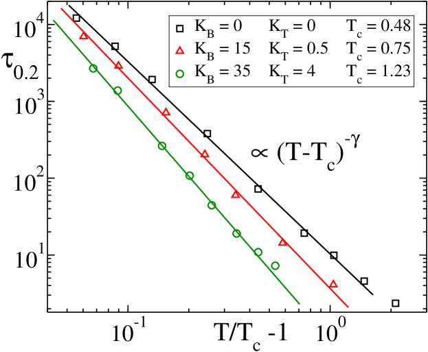
Fig. 17 shows, for the same values of $(K_{\rm B},K_{\rm T})$ in Fig. 16, a test of the power law $\tau_{0.2}\propto(T-T_{\rm c})^{-\gamma}$ for the temperature dependence of the estimated $\alpha$-relaxation times. The fit covers about three time decades. By representing the data in terms of the separation parameter $T/T_{\rm c}-1$, clearly different $\gamma$-exponents are evidenced for different barrier strength. A good description of the data is obtained with the $\gamma$-values derived, through Eqs. (35, 40), from the $b$-values used in Figs. 14 and 16. This result demonstrates the consistency of the MCT analysis for the representative examples showed here, which cover all the range of investigated barrier strength between fully-flexible and stiff chains.

	$\rho$		$K_{\rm B}$		$K_{\rm T}$		$R_{\rm ee}^{\rm c}$		$T_{\rm c}$		$\lambda$
	1		0		0		3.6		0.48		0.761
	1		4		0.1		4.4		0.54		0.767
	1		8		0.2		4.7		0.67		0.773
	1		15		0.5		5.2		0.75		0.785
	1		25		1		5.5		0.82		0.827
	1		25		4		6.4		1.02		0.845
	1		35		4		6.5		1.23		0.862
	0.93		35		4		6.9		1.02		0.885

Table 1: Values of the MCT $\lambda$-exponents and critical temperatures $T_{\rm c}$ for different $\rho$ and barrier strength. Also included are the mean chain end-to-end radii $R_{\rm ee}^{\rm c}$ at $T_{\rm c}$.

Similar consistent tests (not shown) have been performed for the rest of investigated systems. Table 1 displays the results for the so-obtained $\lambda$-exponents and critical temperatures $T_{c}$ as a function of $(K_{\rm B},K_{\rm T})$. We also include the corresponding value of the mean end-to-end radius (computed at $T_{\rm c}$), which provides a qualitative characterization of chain stiffness. From the numerical values in Table 1 a clear correlation between the strength of the internal barriers and the values of $T_{\rm c}$ and $\lambda$ is unambiguously demonstrated. The interplay between packing effects and intramolecular barriers induces a progressive increase of $T_{\rm c}$ at fixed density. A similar effect is observed for the $\lambda$-exponent, which increases from $\lambda=0.761$ for fully-flexible chains to $\lambda=0.885$ for the stiffest investigated chains. The smallest $\lambda$-values in Table 1 are typical of simple glass-formers as the archetype hard-sphere fluid ($\lambda=0.74$) franosch where dynamic arrest is driven by packing effects. The largest ones, $\lambda\lesssim 0.9$, are similar to those observed in realistic models of polymer melts which incorporate the chemical structure of the chains. Some examples include poly(vinyl methylether) capponi , polybutadiene narros1 or poly(vinyl ethylene) narros2 , with respective values of $\lambda=$ 0.87, 0.93, and 0.93.

Thus, the analysis presented here rationalizes the difference in the MCT exponents between fully-flexible bead-spring models and real polymers. The systematic study performed by tuning the barrier strength suggests that large $\lambda$-exponents in real polymers arise from the interplay between two distinct mechanisms for dynamic arrest. These are general packing effects and polymer-specific intramolecular barriers. Large $\lambda$-values arising from the interplay between distinct arrest mechanisms have been observed in systems of very different nature, as short-ranged attractive colloids sperl ; dawson ; zaccarelli (competition between hard-sphere repulsion and short-ranged reversible bonding), polymer blends blends1 ; blends2 and colloidal mixtures with strong dynamic asymmetry mixtures1 ; mixtures2 (bulk-like caging and matrix-induced confinement), or densified silica voigtsildens (presumably bonding and packing). Numerical solutions of the MCT equations in short-ranged attractive colloids sperl ; dawson and quenched-annealed mixtures krakoviack have revealed the existence of higher-order MCT transitions, which are characterized by the upper limit $\lambda=1$. Whether higher-order MCT transitions are present at some region of the control parameter space of the investigated model is an open question.

In this section we have performed a phenomenological analysis of the simulation data within the framework of MCT. In the next section the observed trends are compared with numerical solutions of the MCT equations.

VII. SOLUTION OF THE MCT EQUATIONS

We have solved Eqs. (22) and (23) for the nonergodicity parameters, for all the investigated range of barrier strength. In analogy with the procedure exposed in, e.g., Refs. franosch ; fuchspre , the integrals over the reciprocal space in the corresponding MCT functionals of Eqs. (22) and (24) are discretised to a grid of $M=600$ equispaced points, with $q$-spacing $\Delta q=0.1$, leading to the expressions:

$$\frac{f_{q}}{1-f_{q}}=\frac{\rho(\Delta q)^{3}}{32\pi^{2}}\sum_{x_{k}}\sum_{x_{p}}^{\prime}\frac{x_{k}x_{p}}{x_{q}^{5}}S(q)S(k)S(p)$$

$$\times[(x_{q}^{2}+x_{k}^{2}-x_{p}^{2})c(k)+(x_{q}^{2}+x_{p}^{2}-x_{k}^{2})c(p)]^{2}f_{k}f_{p}$$ (46)

and

$${\cal F}_{ab}^{s}(q)=\frac{\rho(\Delta q)^{3}}{16\pi^{2}}\sum_{x=1}^{N}\omega_{ax}(q)\times$$

$$\sum_{x_{k}}\sum_{x_{p}}^{\prime}\frac{x_{k}x_{p}}{x_{q}^{5}}S(p)[(x_{q}^{2}+x_{p}^{2}-x_{k}^{2})c(p)]^{2}f_{xb}^{s}(k)f_{p}.$$ (47)

In these expressions the wavevectors are defined as $q=x_{q}\Delta q$, $k=x_{k}\Delta q$, and $p=x_{p}\Delta q$, with $x_{q},x_{k},x_{p}=1/2,3/2,...1199/2$. The prime at the sums over $x_{p}$ means that the latter are restricted to $x_{p}$-values following the condition $|x_{q}-x_{k}|+1/2\leq x_{p}\leq x_{q}+x_{k}-1/2$.

The solutions of Eq. (46) are found by a standard iterative procedure $f_{q}^{j+1}/[1-f_{q}^{j+1}]={\cal F}_{q}(\{f^{j}\})$, with $j$ the iteration step, and with the initial condition $f_{q}^{0}=1$. It can be demonstrated that the stability matrix in Eq. (30) has always a maximum non-degenerate eigenvalue $E\leq 1$, which takes the upper value $E_{\rm c}=1$ at the critical point franosch . Thus, by following the drift of $E$ with changing temperature it is possible to bracket the values of the critical nonergodicity parameters $f^{\rm c}_{q}$, and the critical temperature $T_{\rm c}$, with very high precision. Once the values of $f^{\rm c}_{q}$ are obtained, they are fixed in the functional of Eq. (47), and a small number of iterations is needed to find the corresponding critical values $f^{\rm sc}_{ab}(q)$. Finally, the critical nonergodicity parameters for self-correlations are obtained as $f^{\rm sc}_{q}=N^{-1}\sum_{a=1}^{N}f^{\rm sc}_{aa}(q)$.

Following the procedure exposed above, we solved Eq. (46) by inserting as external inputs the structural quantities, $S(q)$ and $c(q)$, as directly computed from the simulations. However, as previously reported in Ref. chongpre for fully-flexible chains, a MCT transition was not observed for any of the investigated barrier strength. This means that the theoretical critical temperature $T_{\rm c}$ is below the lowest simulation temperature for which equilibration was possible. This result is different from the usual observation in non-polymeric systems, for which the theoretical critical point is accessible in simulation time scales. The reason of this difference is, in some way, related with the unability to crystallize of bead-spring models, which avoids a fast growing of peaks under cooling in the static structure factor $S(q)$, leading to MCT kernels which are not sufficiently strong to provide nonzero solutions of $f_{q}$.

Figure 18: Comparison of the critical nonergodicity parameters $f_{q}^{\rm c}$ (top) and $f_{q}^{\rm sc}$ (bottom) obtained from MCT calculations (solid lines) with those obtained from the phenomenological analysis of the simulation data (symbols, dashed lines are guides for the eyes). Results are shown both for fully-flexible chains and for representative stiff chains with $(K_{\rm B},K_{\rm T})=(15,0.5)$.

Figure 19: Critical temperature $T_{\rm c}$ as a function of the end-to-end radius $R_{\rm ee}^{\rm c}$. The theoretical $T_{\rm c}^{\rm MCT}$, as obtained by solving the MCT equations, is compared with the $T_{\rm c}^{\rm MD}$ from the phenomenological analysis of the simulation data.

Since static correlations computed from our equilibrium simulations do not induce a MCT transition, we are forced to use a structural theory for estimating $S(q)$ and $c(q)$ at lower temperatures, which will allows us to insert them in the MCT equations and to search for the critical temperature. Thus, we solve numerically the PRISM equation

$$\rho c(q)=1/\omega(q)-1/S(q),$$ (48)

with the Percus-Yevick (PY) closure relation hansen for the non-bonded potential $V(r)$ of Eq. (1). The PY relation is given by:

$$c(r)=[1-\exp(V(r)/k_{B}T)](h(r)+1),$$ (49)

where $c(r)$ and $h(r)$ are the Fourier transforms in the real space of $c(q)$ and $h(q)$. The coupled set of nonlinear equations (48,49) is solved by a standard Picard iteration method notegridpicard for the quantity $\Gamma(r)=h(r)-c(r)$, which is a smooth function over all the range of $r$. The form factor $\omega(q)$ is an external input in this procedure. We observed (see above) that $\omega(q)$ exhibits a very weak temperature dependence in comparison to the total static structure factor $S(q)$. Thus we just use for each barrier strength the $\omega(q)$, as computed from the simulations, at the lowest temperature for which equilibration was possible.

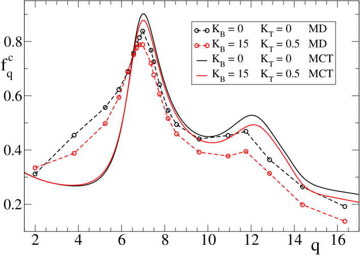
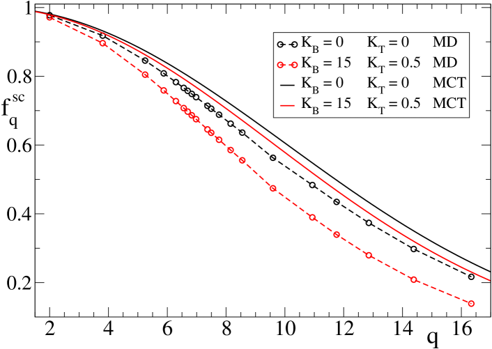
In Fig. 18 we show a comparison of the critical nonergodicity parameters $f^{\rm c}_{q}$ (top panel) and $f^{\rm sc}_{q}$ (bottom panel) as obtained from numerical solution of the MCT equations, with the results of the fitting procedure of simulation data (see above). The theoretical results qualitatively reproduce the simulation trends, and in particular the observation that at fixed density the intramolecular barriers induce a weaker localization length. Quantitatively, the MCT solutions overstimate the amplitude of the nonergodicity parameters, except in the low-$q$ region of $f_{q}^{\rm c}$, for which MCT clearly understimates the results.

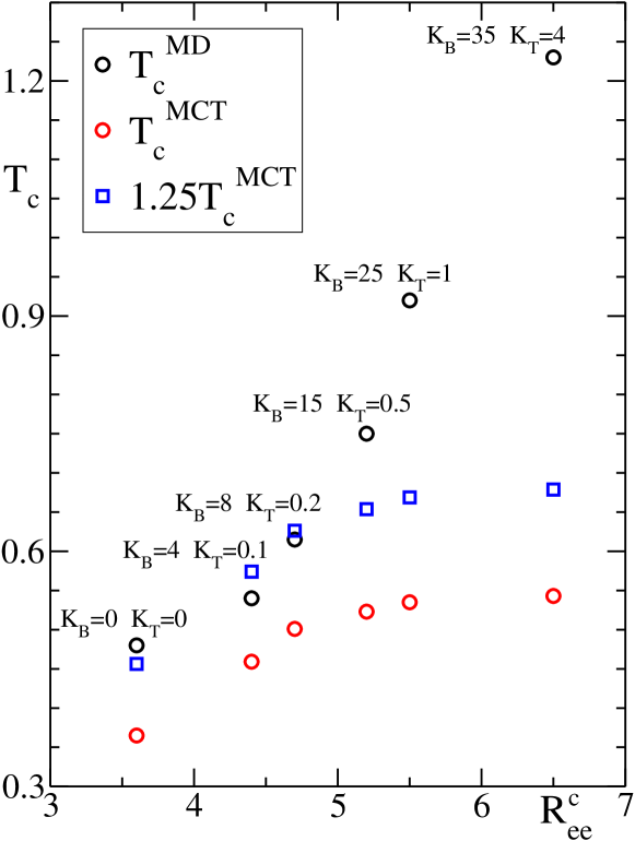
In figure 19 we show a representation of the critical temperature $T_{\rm c}$ as a function of the end-to-end radius $R_{\rm ee}^{\rm c}$, which quantifies chain stiffness. Values of $T_{\rm c}$ obtained from the phenomenological analysis of the simulations ($T_{\rm c}^{\rm MD}$) and from the numerical solutions of the MCT equations ($T_{\rm c}^{\rm MCT}$) are compared. We note that $T_{\rm c}^{\rm MD}$ seems to grow monotonously with chain stiffness. This trend is well reproduced by the theory for low and moderate values of the internal barriers. Thus, for values of bending and torsional constants $K_{B}<15$ and $K_{T}<0.5$, the dependence of $T_{\rm c}^{\rm MCT}$ on $R_{\rm ee}^{\rm c}$ roughly displays the same slope as for $T_{\rm c}^{\rm MD}$, with a shift factor $T_{\rm c}^{\rm MD}/T_{\rm c}^{\rm MCT}\approx 1.25$. Similar shifts between simulation and theory, which have their origin in the mean-field character of the MCT, are observed in other systems vanmegen ; puertas ; sciortino . The range of barrier strength for which $T_{\rm c}^{\rm MCT}$ and $T_{\rm c}^{\rm MD}$ are roughly parallel is significant. Note that for $(K_{\rm B},K_{\rm T})=(8,0.2)$ the end-to-end radius $R_{\rm ee}^{\rm c}$ is a factor 1.3 longer than for fully-flexible chains.

By further increasing chain stiffness the differences between $T_{\rm c}^{\rm MD}$ and $T_{\rm c}^{\rm MCT}$ progressively increase. We observe a saturation of the theoretical $T_{\rm c}^{\rm MCT}$ around $\approx 0.55$, while the simulation $T_{\rm c}^{\rm MD}$ grows up to a value of 1.23 for the stiffest investigated chains. Thus, the agreement between theory and simulation clearly breaks for stiff chains.

Finally, we have computed the corresponding theoretical $\lambda$-exponents according to the definitions of Eqs. (29,30,31). We find an almost constant value of $\lambda\approx 0.72$ for all the investigated range of barrier strength. This result is clearly different from the observations in the phenomenological MCT analysis of simulation data (see data in Table 1), which provides a strong dependence of $\lambda$ on the barrier strength.

VIII. DISCUSSION

The results reported in the previous section show that, though reproducing some qualitative simulation trends for low and moderate barriers, numerical solutions of the MCT equations exhibit important differences with simulation values as the limit of stiff chains is approached. Another result to be understood is the clear disagreement between the almost constant value of the theoretical $\lambda$-exponent, and the observed strong dependence of simulation values on the barrier strength.

The observed disagreement between theory and simulation for strong barriers does not seem to be related with the failure of the PRISM approximations for stiff chains, which have been introduced in the derivation of the MCT equations. Indeed we have shown that the quality of the used PRISM approximations is the same for fully-flexible and stiff chains (Figs. 4, 5 and 6). Having said this, it might be argued that the theory is simply wrong: the phenomenological MCT analysis is apparently successful, but one finds that it has little to do with the theory, for stiff chains, when solving the MCT equations. However, we remind that the phenomenological analysis has shown, for all the investigated range of barrier strength: i) the validity of the two MCT universalities, i.e., the factorization theorem (Figs. 11 and 12) and the TTSP (Fig. 13) ii) the possibility of a good description of different dynamic observables (Figs. 14, 16 and 17) with a set of dynamic exponents which are consistently transformed, through Eqs. (35,40), to a single $\lambda$-exponent.

We believe that all these observations, for all the investigated cases, are not fortuitous. At this point it must be noted that the predictions referred to in points i) and ii) arise, within MCT, as a consequence of the mathematical structure of the equations of motion, more precisely they originate from the bilinear form of the memory kernel. The specific values of the numerical solutions clearly depend on the coefficients of the bilinear products (which enter through the vertices of the kernel), but the factorization theorem, the TTSP, and the asymptotic scaling laws are universal properties provided the kernel is bilinear. Thus, the results of the phenomenological analysis suggest that the underlying physics may be connected to a bilinear memory kernel, though for high barriers the actual coefficients strongly differ from those introduced by MCT through the vertices, thus leading to theoretical results which strongly differ from simulations.

In other words, the present results suggest that there may be relevant static contributions for the case of stiff chains which are missing in the MCT vertices. Thus, the inclusion of such contributions will increase the strength of the kernel and will induce the theoretical transition at higher values of $T_{\rm c}$, which might improve the comparison between $T_{\rm c}^{\rm MCT}$ and $T_{\rm c}^{\rm MD}$ of Fig. 19. Recalling the three main approximations of MCT, we suggest that the convolution approximation, Eq. (16), might break for stiff chains. Though possibly it is not the case for intermolecular contributions, its breakdown for intramolecular contributions in stiff chains is plausible. It is known that the convolution approximation fails when static correlations show a strong directionality at near-neighbor distances, as for e.g., network-forming liquids as silica silicac3 . This directionality is clearly enhanced for intrachain correlations by increasing the barrier strength, as evidenced by the progressively larger values of the end-to-end radius (see Table 1). For the case of silica, it has been shown that the explicit inclusion of three-point static correlations in the MCT vertex improves significantly the quality of the comparison between theory and simulations silicac3 . A similar improvement might be achieved in the present case by similarly incorporating the intrachain three-point static contributions. Work in this direction is in progress.

IX. CONCLUSIONS

We have performed simulations on a simple bead-spring model for polymer melts with intramolecular barriers. The role of such barriers on the glass transition has been investigated by systematically tuning the barrier strength. Dynamic correlators probing the structural relaxation have been analyzed in the framework of the Mode Coupling Theory. We have obtained critical nonergodicity parameters, critical temperatures and dynamic exponents of the theory from consistent fits of simulation data to MCT asymptotic laws. From the analysis of the critical nonergodicity parameters we deduce that the presence of the barriers induces a weaker localization length in the system at fixed density. The increase of the barrier strength at fixed density also induces a higher critical temperature $T_{\rm c}$. The values of the dynamic exponents, as obtained from the phenomenological analysis of the simulation data, exhibit significant differences between the limit of fully-flexible and stiff chains. In particular the so-called $\lambda$-exponent takes standard values $\lambda\sim 0.7$ for the fully-flexible case and values approaching the upper limit $\lambda=1$ for strong intramolecular barriers. While the former $\lambda$-values are characteristic of simple systems dominated by packing effects, transitions with $\lambda\approx 1$ arise in systems with different competing mechanisms for dynamic arrest. In our systems these large $\lambda$-values suggest a competition between two distinct mechanisms: general packing effects and polymer-specific intramolecular barriers.

For a comparison between simulation and theory, we have numerically solved the MCT equations, following a recent extension of the MCT by Chong and co-workers for polymer melts. The approximations assumed by the structural PRISM theory, which are introduced in the MCT equations, are fulfilled for all the investigated values of the barrier strength. We have compared the critical nonergodicity parameters and critical temperatures $T_{\rm c}$, as obtained by solving the MCT equations, with the corresponding values from the phenomenological analysis of the simulation data. The theoretical calculations qualitatively reproduce the trends observed in the simulations for low and moderate barriers. However strong discrepancies are observed as the limit of high barriers is approached. The reason for such a disagreement possibly lies in the nature of the approximations made in the derivation of the MCT equations. In particular, the convolution approximation for three-point static correlations might be unadequate for stiff chains. We suggest that a reformulation of MCT equations for polymer melts, explicitly including intrachain three-point static correlations, might lead to a better agreement between simulations and theory. Work in this direction is in progress.

ACKNOWLEDGEMENTS

We acknowledge financial support from the projects NMP3-CT-2004-502235 (SoftComp, EU), MAT2007-63681 (Spain), 2007-60I021 (Spain), and IT-436-07 (GV, Spain). We thank S.-H. Chong, E. Zaccarelli, M. Fuchs and M. Sperl for useful discussions.

References

- (1) M. Doi and S. F. Edwards, The theory of Polymer Dynamics, (Oxford University Press, Oxford, 1986).
- (2) P. G. de Gennes, Scaling Concepts in Polymer Physics, (Cornell University Press, Ithaca, London, 1979).
- (3) T.C.B. McLeish, Adv. Phys. 51, 1379 (2002).
- (4) J. Colmenero, A.J. Moreno, and A. Alegría, Prog. Polym. Sci. 30, 1147 (2005).
- (5) H. Meyer and F. Müller-Plathe, Macromolecules 35, 1241 (2002).
- (6) T. Vettorel, H. Meyer, J. Baschnagel, and M. Fuchs, Phys. Rev. E 75, 041801 (2007).
- (7) R. Faller and F. Müller-Plathe, Chem. Phys. Chem. 3, 180 (2001).
- (8) M. Bulacu and E. van der Giessen, J. Chem. Phys. 123, 114901 (2005).
- (9) C. Bustamante, J. Marko, E. Siggia, and S. Smith, Science 265, 1599 (1994).
- (10) J. Käs, H. Strey, J.X. Tang, D. Finger, R. Ezzell, E. Sackmann, P.A. Janmey, Biophys. J. 70, 609 (1996).
- (11) C. K. Ober, Science 288, 448 (2000).
- (12) A.N. Semenov, Eur. Phys. J. E 9, 353 (2002).
- (13) J. Ubbink and A. Khokhlov J. Chem. Phys. 120, 5353 (2004).
- (14) W. Götze and L. Sjögren, Rep. Prog. Phys. 55, 241 (1992).
- (15) W. Götze, J. Phys.: Condens. Matter 11, A1 (1999).
- (16) W. Götze, in Liquids, Freezing and Glass Transition, edited by J.-P. Hansen, D. Levesque, and J. Zinn-Justin (North-Holland, Amsterdam, 1991).
- (17) D. R. Reichman and P. Charbonneau, J. Stat. Mech., P05013 (2005).
- (18) S.P. Das, Rev. Mod. Phys. 76, 785 (2004).
- (19) W. Götze, Complex Dynamics of Glass-Forming Liquids. A Mode Coupling Theory, (Oxford University Press, New York, 2009).
- (20) M. Bernabei, A. J. Moreno, J. Colmenero, Phys. Rev. Lett. 101, 255701 (2008).
- (21) W. Götze and M. Sperl, Phys. Rev. E 66, 011405 (2002).
- (22) M. Sperl, Phys. Rev. E 68, 031405 (2003).
- (23) V. Krakoviack, Phys. Rev. E 75, 031503 (2007); ibid. 79, 061501 (2009).
- (24) S.-H. Chong and M. Fuchs, Phys. Rev. Lett. 88, 185702 (2002).
- (25) S.-H. Chong, M. Aichele, H. Meyer, M. Fuchs, J. Baschnagel, Phys. Rev. E 76, 051806 (2007).
- (26) K.S. Schweizer, E.F. David, C. Singh, J.G. Curro, J.J. Rajasekaran, Macromolecules 28, 1528 (1995).
- (27) K. S. Schweizer and J. G. Curro, Adv. Chem. Phys. 98, 1 (1997).
- (28) M. Pütz, J. G. Curro, and G. S. Grest, J. Chem. Phys. 114, 2847 (2001).
- (29) G. S. Grest and K. Kremer, Phys. Rev. A 33, R3628 (1986).
- (30) C. Bennemann, J. Baschnagel, and W. Paul, Eur. Phys. J. B 10, 323 (1999).
- (31) M. Bulacu and E. van der Giessen, Phys. Rev. E 76, 011807 (2007).
- (32) D. Frenkel and B. Smit, Understanding Molecular Simulation (Academic Press, San Diego, 1996).
- (33) D. Chandler and H.C. Andersen, J. Chem. Phys. 57, 1930 (1972).
- (34) M. Aichele, S.-H. Chong, J. Baschnagel, M. Fuchs, Phys. Rev. E 69, 061801 (2004).
- (35) M. Aichele and J. Baschnagel, Eur. Phys. J. E 5, 229 (2001); ibid. 5, 245 (2001).
- (36) T. Franosch, M. Fuchs, W. Götze, M. R. Mayr, and A. P. Singh, Phys. Rev. E 55, 7153 (1997).
- (37) M. Fuchs, W. Götze, and M. R. Mayr, Phys. Rev. E 58, 3384 (1998).
- (38) J. P. Hansen and I. R. McDonald, Theory of Simple Liquids, 2nd ed. (Academic Press, London, 1986).
- (39) S.-H. Chong and F. Hirata, Phys. Rev. E 58, 6188 (1998); ibid. 58, 7296 (1998).
- (40) In reality, it is well-known that hopping events, not accounted for within the ideal version of MCT here described, restore ergodicity and the MCT transition does not really occur. Indeed is found to be higher than the actual ‘laboratory’ glass transition of the system. Having said this, the MCT asympotic laws (see main text) for dynamic correlators and relaxation times by approaching usually hold for not too small values of the separation parameter .
- (41) S.-H. Chong, W. Götze, and A.P. Singh, Phys. Rev. E 63, 011206 (2000).
- (42) M. Fuchs, J. Non-Cryst. Solids 172, 241 (1994).
- (43) W. van Megen and S.M. Underwood, Phys. Rev. Lett. 70, 2766 (1993).
- (44) W. Kob and H.C. Andersen, Phys. Rev. E 52, 4134 (1995).
- (45) J. Baschnagel and F. Varnik, J. Phys.: Condens. Matter 17, R851 (2005).
- (46) S. Capponi, A. Arbe, F. Alvarez, J. Colmenero, B. Frick, J.P. Embs, submitted.
- (47) J. Colmenero, A. Narros, F. Alvarez, A. Arbe, A.J. Moreno, J. Phys.: Condens. Matter 19, 205127 (2007).
- (48) A. Narros, Ph.D. thesis, Universidad del País Vasco (UPV/EHU), 2007.
- (49) K. Dawson, G. Foffi, M. Fuchs, W. Götze, F. Sciortino, M. Sperl, P. Tartaglia, Th. Voigtmann, and E. Zaccarelli, Phys. Rev. E 63, 011401 (2000).
- (50) E. Zaccarelli, G. Foffi, K.A. Dawson, S.V. Buldyrev, F. Sciortino, and P. Tartaglia, Phys. Rev. E 66, 041402 (2002).
- (51) A. J. Moreno and J. Colmenero, J. Chem. Phys 124, 184906 (2006).
- (52) A. J. Moreno and J. Colmenero, J. Phys.: Condens. Matter 19, 466112 (2007).
- (53) A. J. Moreno and J. Colmenero, Phys. Rev. E 74, 021409 (2006).
- (54) A. J. Moreno and J. Colmenero, J. Chem. Phys 125, 164507 (2006).
- (55) T. Voigtmann and J. Horbach, J. Phys.: Condens. Matter 20, 244117 (2008).
- (56) Fast Fourier tranforms are used to switch back and forth between the - and -space. We use a grid of equispaced points from to in the real space. For the reciprocal space we use points from to . We use the criterion for convergence . The iteration is performed by mixing the old solution with the current in order to obtain the new solution , according to .
- (57) T. Voigtmann, A.M. Puertas, and M. Fuchs, Phys. Rev. E 70, 061506 (2004).
- (58) F. Sciortino, P. Tartaglia, and E. Zaccarelli, Phys. Rev. Lett. 94, 065703 (2005).
- (59) F. Sciortino and W. Kob, Phys. Rev. Lett. 86, 648 (2001).