Non-ideal behavior of intramolecular structure factor of dilute polymers in a theta solvent

Abstract

We study the configurational properties of single polymers in a theta solvent by Monte Carlo simulation of the bond fluctuation model. The intramolecular structure factor at the theta point is found to be distinctively different from that of the ideal chain. The structure factor shows a hump around $q\sim 5/R_{g}$ and a dip around $q\sim 10/R_{g}$ in the Kratky plot with $R_{g}$ being the radius of gyration. This feature is apparently similar to that in a melt. The theoretical expression by the simple perturbation expansion to the first order in terms of the Mayer function can be fitted to the obtained structure factor quite well, but the second virial coefficient cannot be set to zero.

I Introduction

One of the basic premises in the polymer physics is that the bonds connecting neighboring monomer units are uncorrelated beyond the persistent length along the chain De Gennes (1979). This property allows us to consider only a flexible chain as long as we are interested in large scale properties of a polymer chain that is much longer than its persistent length. In this sense, it was a little embarrassing to realize that there is actually a long range correlation in the bond orientation of a polymer chain, and that the bond-bond correlation function decays not exponentially but as the power law Schäfer et al. (1999); Schäfer and Elsner (2004); Wittmer et al. (2004).

The traditional picture for the bond-bond correlation is based on a simple calculation for the polymer with a fixed bond angle around freely rotating bonds. In this case, one can calculate the bond-bond correlation function explicitly to show the exponential decay with a persistent length Flory (1988). The existence of the long range correlation, however, has been pointed out Schäfer et al. (1999); Schäfer and Elsner (2004), and it was demonstrated recently that the power law behavior is induced in the bond-bond correlation through the interaction between monomers separated by a long distance in the curvilinear coordinate along the chain Wittmer et al. (2004); Wittmer et al. (2007a, b); Beckrich et al. (2007); Shirvanyants et al. (2008). The power law in the bond-bond correlation holds not only for an excluded volume chain, but also for a chain in a melt and in a theta solvent, where a polymer chain is supposed to behave as an ideal chain Flory (1988); De Gennes (1979). This has been confirmed both by numerical simulations and by theoretical analyses.

This deviation from the ideality of a chain in a melt has been seen also in the intramolecular structure factor. For the ideal chain, the structure factor decays as $q^{-2}$ in the intermediate range, $1/R_{g}\lesssim q\ll 1/a$, where $R_{g}$ and $a$ are the gyration radius and the bond length, respectively. This $q^{-2}$ decay comes from the fractal dimension of the ideal chain configuration. The intramolecular structure factor of the polymer chain in a melt has been studied numerically and theoretically, and it has been found that there exists a substantial deviation from the ideal chain behavior Beckrich et al. (2007).

In this paper, we study the structure factor of a single polymer molecule in a theta solvent, that is another situation where a polymer chain is supposed to become ideal effectively. In a melt, the interaction between monomers is screened by the existence of other polymer chains, and the excluded volume effect is canceled exactly by the induced attraction due to the incompressibility of the system Flory (1988); Doi and Edwards (1986) while the interaction in a theta solvent is being adjusted by some fine tuned external parameter, such as temperature, so that the excluded volume effect is compensated by the attractive part of the interaction. We study how this fine tuning of the parameter may affect on the virtual ideality of the structure factor.

This paper is organized as follow. After quickly reviewing how the long range correlation comes into the bond-bond correlation in Sec.2, the model and the method of our simulations are described in Sec.3, and the simulations results are given in Sec.4. The theoretical analysis is outlined in Sec.5 and the results are discussed in connection with those for melt in Sec.6. Detailed expressions of the theoretical analysis are given in Appendix.

II Bond-bond correlations in a polymer chain

Let us quickly review how the long range correlation should arise in the bond-bond correlation along a polymer chain Wittmer et al. (2004). We consider a single polymer that consists of $N$ monomers. Let $\mbox{\boldmath$r$}_{n}$ ($n=1,\cdots,N$) be the position of the $n$-th monomer in it, and the bond vector is denoted as

$$\mbox{\boldmath$a$}_{n}\equiv\mbox{\boldmath$r$}_{n+1}-\mbox{\boldmath$r$}_{n}.$$ (1)

We define a subchain as a part of the chain, and introduce the subchain vector as

$$\mbox{\boldmath$R$}_{n}(s)\equiv\mbox{\boldmath$r$}_{n+s}-\mbox{\boldmath$r$}_{n}=\sum_{r=n}^{n+s-1}\mbox{\boldmath$a$}_{r}.$$ (2)

Now, we assume that the bond-bond correlation depends only on the chemical distance between the bonds:

$$P(s)={1\over a^{2}}\left<\mbox{\boldmath$a$}_{n}\cdot\mbox{\boldmath$a$}_{n+s}\right>,$$ (3)

where $a$ is the average bond length and $\left<\cdots\right>$ denotes the ensemble average. Then, the size of the subchain does not depend on $n$, and we have

$$R(s)^{2}\equiv\left<\mbox{\boldmath$R$}_{n}(s)^{2}\right>\approx a^{2}\left(s+\int_{0}^{s}dr(s-r)P(r)\right)$$ (4)

in the large $s$ approximation. This gives

$$P(s)\approx{1\over a^{2}}\,{\partial^{2}\over\partial s^{2}}R(s)^{2}\sim s^{-\omega}$$ (5)

with $\omega=2-2\nu$ if the subchain size scales as

$$R(s)\sim s^{\nu}$$ (6)

with the exponent $\nu\neq 1/2$. We have $\omega\approx 0.824$ for the excluded volume chain, where $\nu\approx 0.588$.

For the ideal chain with $\nu=1/2$, Eq.(5) gives $P(s)=0$ as it should, but for the case of apparent ideality of a polymer chain in a melt or a theta solvent, we have

$$P(s)\sim s^{-3/2}$$ (7)

because of the correction term,

$$R(s)^{2}\approx a^{2}s\left(c_{0}+c_{1}\,s^{-1/2}+\cdots\right).$$ (8)

III Model and Simulation Method

We perform Monte Carlo simulations of the bond fluctuation model (BFM) on the three dimensional cubic lattice Carmesin and Kremer (1988); Deutsch and Binder (1991). A polymer chain consists of $N$ monomers, and the $i$-th monomer is located at the center of a cubic cell $\mbox{\boldmath$r$}_{i}$, occupying the cell with 8 vertices at lattice sites. The bond length between consecutive monomers along the chain should be in the range $[2,\sqrt{10}]$ with the exception of $\sqrt{8}$. The $i$-th and $j$-th monomers that are not consecutive along the chain, namely $j\neq i\pm 1$, interact each other through the “quasi-Lennard-Jones” potential energy Ivanov et al. (1998)

$${U(r_{ij})\over k_{B}T}=\left\{\begin{array}[]{l}-\beta\Bigl{(}2(r_{ij}-2)^{3}-3(r_{ij}-2)^{2}+1\Bigr{)}\\ \hfill\mbox{for }r_{ij}=2,\sqrt{5},\sqrt{6},\mbox{ and }\sqrt{8}\\ 0\\ \hfill\qquad\mbox{otherwise }\end{array}\right.,$$ (9)

where $r_{ij}=|\mbox{\boldmath$r$}_{i}-\mbox{\boldmath$r$}_{j}|$ is the distance between the interacting monomers, and $k_{B}$ and $T$ are the Boltzmann constant and the temperature, respectively. The dimensionless parameter $\beta$ is proportional to the inverse temperature and characterizes the interaction com .

We perform Monte Carlo simulations, using Metropolis method along with the slithering snake algorithm to accelerate the relaxation towards equilibrium Wall and Mandel (1975). In our system, there is only one polymer chain with $N$ monomer units. One Monte Carlo step consists of $N$ trials of random displacement to one of the nearby sites for randomly chosen monomers, followed by $N$ slithering snake trials.

The quantities we study are the radius of gyration $R_{g}$,

$$R_{g}^{2}\equiv\left<{1\over 2N^{2}}\sum_{i=1}^{N}\sum_{j=1}^{N}(\mbox{\boldmath$r$}_{i}-\mbox{\boldmath$r$}_{j})^{2}\right>,$$ (10)

the intrachain structure factor $S(\mbox{\boldmath$q$})$,

$$S(\mbox{\boldmath$q$})\equiv\left<{1\over N}\sum_{i=1}^{N}\sum_{j=1}^{N}e^{i\mbox{\boldmath$q$}\cdot(\mbox{\boldmath$r$}_{i}-\mbox{\boldmath$r$}_{j})}\right>,$$ (11)

and the bond-bond correlation $P(s)$ averaged over the chain,

$$P(s)\equiv{1\over a^{2}(N-1-s)}\sum_{i=1}^{N-1-s}\left<\mbox{\boldmath$a$}_{i}\cdot\mbox{\boldmath$a$}_{i+s}\right>$$ (12)

with the average bond length $a$,

$$a^{2}\equiv\left<{1\over N-1}\sum_{i=1}^{N-1}\mbox{\boldmath$a$}_{i}^{2}\right>,$$ (13)

where the angular brackets represent the ensemble average.

Note that the radius of gyration can be expressed using the bond-bond correlation by a similar equation as Eq.(4):

$$R_{g}^{2}\approx{1\over 6}a^{2}N\left[1+\int_{0}^{N}dr\left(1-{r\over N}\right)^{3}P(r)\right].$$ (14)

IV Results

IV.1 Theta Point

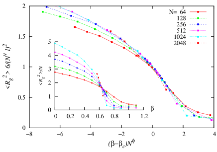
Figure 1: (Color online) The scaling plot for the radius of gyration $R_{g}$. The scaled radius of gyration $R_{g}^{2}\,6/(N^{\nu}\ell)^{2}$ are plotted against $(\beta-\beta_{c})N^{\phi}$ with $\beta_{c}=0.63$, $\nu=\phi=$ 0.5, and $\ell=3.17$ for various values of $N$ The inset shows the original plot of $R_{g}^{2}/N$ vs $\beta$.

First, we have to determined the theta point for our model. It is often defined as the point where the second virial coefficient vanishes. In our simulations, we define the theta point as the point where the radius of gyration $R_{g}$ behaves as an ideal chain,

$$R_{g}\propto\sqrt{N},$$ (15)

in the large $N$ limit. The interaction parameter $\beta_{c}$ at the theta point is determined numerically from the data of $R_{g}$ for various values of $\beta$ and chain length $N$ by fitting them to the finite size scaling form

$$R_{g}^{2}={1\over 6}N^{2\nu}\ell^{2}\,f\left(({\beta-\beta_{c})N^{\phi}}\right)$$ (16)

with the two exponents, $\nu$ and $\phi$. The function $f(x)$ is the scaling function that satisfies $f(0)=1$, and $\ell$ is the length scale proportional to the average bond length. Fig.1 shows that the data fit well to the scaling form (16) with

$$\beta_{c}=0.63,\quad\nu=\phi=1/2,\quad\ell=3.17.$$ (17)

IV.2 Theta Point determined by Bond-Bond Correlation

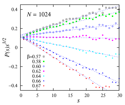
Figure 2: (Color online) Bond-bond correlation. $P(s)s^{3/2}$ are plotted against $s$ for $N=1024$ for various $\beta$.

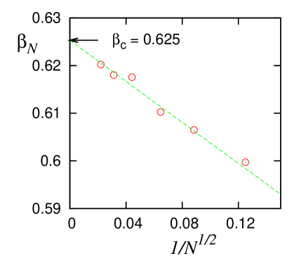
Figure 3: (Color online) The theta point determined by the bond-bond correlation. The values of $\beta$ where the bond-bond correlation shows the ideal behavior, $s^{-3/2}$, are plotted against $1/N^{1/2}$. The linear extrapolation to the infinite $N$ shows the theta point, $\beta_{c}=0.625$.

As we have discussed, the bond-bond correlation function decays as $s^{-3/2}$ at the theta point. Fig.2 shows the bond-bond correlation function $P(s)$ for various temperatures near the theta point for $N=1024$. It shows that the data fit to the form

$$P(s)s^{3/2}=\tilde{B}_{0}\Bigl{(}1-\beta/\beta_{c}(N)\Bigr{)}s+\tilde{A}+\cdots$$ (18)

that is consistent with the theoretical results by Shirvanyants, et al. Shirvanyants et al. (2008). The theta point may be defined as $\beta=\beta_{c}(N)$ where the bond-bond correlation decays as $s^{-3/2}$, but it turns out that $\beta_{c}(N)$ depends on $N$. The $N$-dependence of $\beta_{c}(N)$ plotted in Fig.3 shows

$$\beta_{c}(N)-\beta_{c}\propto{1\over\sqrt{N}}$$ (19)

with the theta point in the infinite $N$ limit $\beta_{c}=0.625$. This value is close enough to the previous estimate of $\beta_{c}=0.63$ by the scaling plot of $R_{g}$. In the rest of the paper, we use $\beta_{c}=0.63$ for the theta point. Note that the $N$-dependence of $\beta_{c}(N)$ given by Eq.(19) is consistent with the ideal chain behavior of $R_{g}$ of Eq.(15) at $\beta=\beta_{c}$ in respect to Eq.(14).

IV.3 Structure Factor

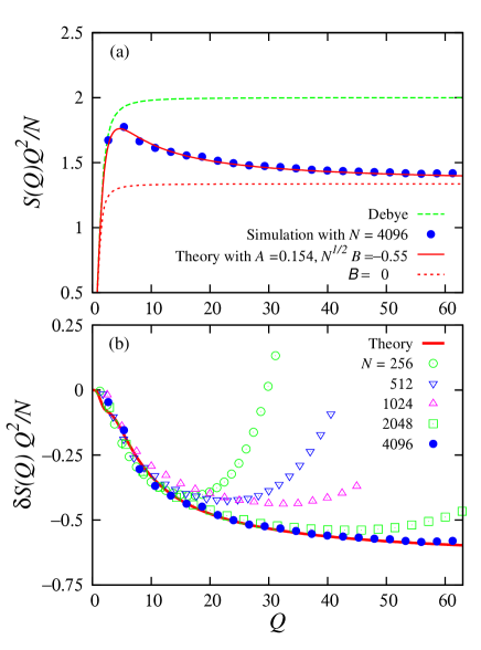
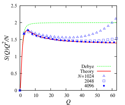
Figure 4: (Color online) Kratky plots for the structure factor against $Q\equiv qR_{g}$. The simulation data at $\beta=0.63$ for the chain with the length $N=$1024, 2048, and 4096 are plotted along with the Debye scattering function (the dashed line). For the value of $R_{g}$, the values obtained by the simulations are used for the simulation data and $R_{g0}=Na^{2}/6$ for the analytical expressions. The red curve represent the theoretical estimate, Eq.(29), with $\sqrt{N}B=-0.55$ and $A=0.154$.

The structure factor for the ideal chain, $S_{0}(q)$, in the large $N$ limit is given by

$$S_{0}(q)=Nf_{D}(qR_{g0})$$ (20)

with the radius of gyration for the ideal chain

$$R_{g0}^{2}\equiv{1\over 6}Na^{2}.$$ (21)

and the Debye scattering function,

$$f_{D}(x)\equiv{2\over x^{4}}\Bigl{(}e^{-x^{2}}-1+x^{2}\Bigr{)}.$$ (22)

In the intermediate length scale, i.e., $1/R_{g0}\ll q\ll 1/a$, this decays as

$$S_{0}(q)\approx{12\over a^{2}}\,q^{-2}+O(q^{-4}).$$ (23)

The $1/q^{2}$-dependence comes from the scaling behavior of the ideal chain, therefore, the existence of plateau in the plot of $S(q)\,q^{2}$, i.e., Kratky plot, has been considered to be a sign of the ideality in a polymer chain behavior.

Fig.4 shows the Kratky plot of our numerical simulations at the theta point for $N=1024\sim 4096$; The wave number $q$ is scaled by the numerically obtained radius of gyration $R_{g}$ as $Q\equiv qR_{g}$. As the number of monomers $N$ increases, the curve in the smaller $Q$ regime tends to converge to a common trend, but it is clearly different from that of the ideal chain (the dashed line). The Kratky plot at the theta point shows a hump around $Q\sim 5$ and a dip around $Q\sim 10$, and does not show the plateau as the one would expect for the ideal chain. Their general features are apparently similar to those found for a polymer chain in a melt Beckrich et al. (2007).

V Theory

Now, we estimate the structure factor theoretically and compare it with those obtained by the simulations. Suppose $u(\mbox{\boldmath$r$}_{s,r})$ be the interaction potential between the $s$-th and the $r$-th monomers with $\mbox{\boldmath$r$}_{s,r}\equiv\mbox{\boldmath$r$}_{s}-\mbox{\boldmath$r$}_{r}$. Then the structure factor Eq.(11) is written as

$$S(\mbox{\boldmath$q$})={2\over N}\sum_{n>m}{\left<e^{i\mbox{\boldmath$q$}\cdot\mbox{\boldmath$r$}_{n,m}}e^{-U/k_{B}T}\right>_{0}\over\left<e^{-U}\right>_{0}}+1,$$ (24)

where

$$U\equiv\sum_{r>s}u(\mbox{\boldmath$r$}_{r,s}),$$ (25)

and $\left<\cdots\right>_{0}$ represents the statistical average for the ideal chain.

We now employ the approximation

$$e^{-U/k_{B}T}\approx 1+\sum_{r>s}f(\mbox{\boldmath$r$}_{r,s})$$ (26)

using the Mayer function

$$f(\mbox{\boldmath$r$}_{r,s})\equiv e^{-u(\mbox{\boldmath$r$}_{r,s})/k_{B}T}-1.$$ (27)

Then up to the first order in $f$, the correction in the structure factor $\delta S(\mbox{\boldmath$q$})$ is given by

$$\delta S(\mbox{\boldmath$q$}) \equiv S(\mbox{\boldmath$q$})-S_{0}(\mbox{\boldmath$q$})$$ (28)

$$\approx {2\over N}\sum_{n>m}\,\sum_{r>s}\Bigl{[}\left<e^{i\mbox{\boldmath$q$}\cdot\mbox{\boldmath$r$}_{n,m}}f(\mbox{\boldmath$r$}_{r,s})\right>_{0}$$

$$\hskip 50.00008pt-\left<e^{i\mbox{\boldmath$q$}\cdot\mbox{\boldmath$r$}_{n,m}}\right>_{0}\left<f(\mbox{\boldmath$r$}_{r,s})\right>_{0}\Bigr{]}.$$

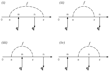
Figure 5: Diagrams that represent contribution for Eq.(28).

There are four types of contribution in Eq.(28) depending upon the relative positions of $n$, $m$, $r$, and $s$ (Fig.5). Adopting the bead-spring model for the ideal chain average $\left<...\right>_{0}$ with the average bond length $a$, and employing the further approximation valid for $qa\ll 1$, we obtain the expression

$${1\over N}\delta S(\mbox{\boldmath$q$})\approx F(qR_{g0})\sqrt{N}B+G(qR_{g0})A$$ (29)

up to the second leading order in $N$. The functional forms for $F$ and $G$ are given in Appendix. The dimensionless parameters,

$$B \equiv -{1\over a^{3}}\int d\mbox{\boldmath$r$}f(\mbox{\boldmath$r$}),$$ (30)

$$A \equiv {1\over a^{5}}\int d\mbox{\boldmath$r$}\,r^{2}f(\mbox{\boldmath$r$}),$$ (31)

characterize the interaction. The parameter $B$ is twice of the second virial coefficient for the unlinked monomer gas Hansen and McDonald (1986), and is supposed to be close to zero for the theta solvent Doi and Edwards (1986). Note that $B$ comes into $S(q)$ as $\sqrt{N}B$.

Figure 6: (Color online) Theoretical results for structure factors. The numerical estimates by Eq.(29) are plotted with $A=0.154$ and $\sqrt{N}B=-0.55$, and 0.

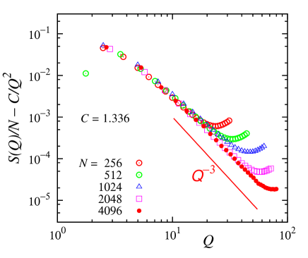
Figure 7: (Color online) The large $Q$ behavior of the structure factor after subtracting $C/Q^{2}$ with $C=1.336$.

Fig.6(a) shows the Kratky plots for the theoretical structure factor $S(Q)Q^{2}$ with $Q\equiv qR_{g0}$ by Eq.(29) with $A=0.154$ and $\sqrt{N}B=-0.55$ along with the curve for $A=0.154$ and $B=0$, the Debye function, and the simulation data for $N=4096$. One can see that the curve for $B=0$ is almost proportional to the Debye function and cannot be fitted to the simulation data. Fig.6(b) shows $\delta S(Q)Q^{2}/N$ with the simulation data for various values of $N$. The data converge to the theoretical curve quite well as $N$ increases.

In Fig.7, the large $Q$ behavior of the structure factor are plotted in the logarithmic scale, after subtracting the leading order term of $C/Q^{2}$ with $C=1.336$. It shows clearly that the second leading order is $1/Q^{3}$, which is consistent with the asymptotic expression we obtained in Eq.(53).

VI Discussions

Our findings are summarized as follows: (i) The theta point for the finite chain $\beta_{c}(N)$, where the bond-bond correlation decays as $s^{-3/2}$, depends on the chain length $N$, and in the infinite chain length limit it converges to the theta point $\beta_{c}$ determined by the scaling behavior of the radius of gyration. (ii) The structure factors at the theta point $\beta_{c}$ obtained by the numerical simulations are distinctively different from that of the ideal chain, i.e., (ii-a) in the intermediate range of $q\gtrsim 1/R_{g}$, Kratky plot of the structure factor shows a hump and a dip, and (ii-b) in the larger $q$ range, $1/R_{g}\ll q\ll 1/a$, the structure factor decays as $1/q^{2}$ with the next order term of $1/q^{3}$. (iii) In the large $N$ limit, numerically obtained structure factors fit well to the simple perturbation expression up to the first order of the Mayer function with the fitting parameters $\sqrt{N}B=-0.55$ and $A=0.154$.

In comparison with the case of a melt, the obtained structure factors at the theta point apparently resemble the ones of a melt in the existence of a hump and a dip Beckrich et al. (2007). In the large $q$ region, however, the structure factors for the two cases differ; In the case of melt, it has been shown by numerical simulations that structure factors decays as $1/q^{3}$ for the large $q$ region Beckrich et al. (2007), in contrast with the present case, where we found the $1/q^{2}$ decay with the positive $1/q^{3}$ correction. The $1/q^{3}$ decay in the melt was interpreted as a result of renormalization from the $1/q$ term obtained by the one-loop approximation Beckrich et al. (2007) while the $1/q^{2}$ term and the $1/q^{3}$ term at the theta point directly correspond to the $A$-term and the $\sqrt{N}B$-term, respectively, in our theoretical expression. In the real space, the $1/q^{2}$ decay of the structure factor in large $q$ means the $1/r$ density correlation of the ideal chain in short $r$. The existence of the positive $1/q^{3}$ correction and the hump around $q\sim 5/R_{g}$ implies that the density correlation does not decay as fast as that of the ideal chain around $r\sim R_{g}$.

The simulated structure factors here at the theta point resemble those of a melt, but it is intriguing that we need to set $\sqrt{N}B\neq 0$ for our theoretical expression of the structure factor to fit to the numerical results at the theta point $\beta_{c}$. The theta point is often considered as the point where the second virial coefficient $B/2$ vanishes. Actually, if we set $B=0$, the structure factor shows Kratky plateau and looks pretty much like the ideal one (the dotted line in Fig.6(a)), but this cannot be fitted to the simulation results by adjusting $A$ alone even with an arbitrary factor. Theoretically, if we consider higher order corrections, the theta point should correspond to the vanishing point of the interaction parameter $z$

$$z\equiv\sqrt{N}b$$ (32)

where $b$ is the excluded volume parameter with the additive renormalization by the higher order cluster contributions, and may be given in the form

$$b=B+CN^{-1/2}+\dots$$ (33)

with a constant $C$. However, such renormalization effect could be partially taken into account by replacing $B$ with $b$, and one would expect the structure factor at the theta point should be given by the one with $\sqrt{N}B=0$ in our expression.

In the bond-bond correlation $P(s)$, we observed the analogous $N$-dependence, which can be interpreted in the same way. Shirvanyants et al. Shirvanyants et al. (2008) have obtained the theoretical expression corresponding to Eq.(18) in a similar approximation to the one we employed for $S(\mbox{\boldmath$q$})$, and showed that the coefficients for the $s^{-1/2}$ and the $s^{-3/2}$ terms in Eq.(18), i.e. $\tilde{B}_{0}(1-\beta/\beta_{c}(N))$ and $\tilde{A}$, are proportional to the parameters $B$ and $A$, respectively. The observed $N$-dependence in $\beta_{c}(N)$ as Eq.(19) in our simulations should be a result of higher order effects, that could be obtained by replacing the coefficient of $s^{-1/2}$-term with the renormalized one as Eq.(33).

Regarding the origin for the deviation of the structure factor from the Debye function, an obvious possibility could be that inaccurate estimate for the theta point $\beta_{c}$, i.e. our estimate $\beta_{c}=0.63$ is not close enough to the theta point for the structure factor to be Debye-like even though the two independent estimates from the radius of gyration $R_{g}$ and the bond correlation coincide with each other within our numerical precision. This might happen due to the slow convergence caused by the logarithmic correction at the theta point. Another possibility, perhaps more interesting one, would be that the tricritical fluctuations at the theta point produce a non-trivial contribution to the structure factor.

Appendix A First oder calculation of $S(\mbox{\boldmath$q$})$ in the Mayer function

In the appendix, we describe the calculation of Eq.(28) to obtain the explicit expressions for $F$ and $G$ in Eq.(29).

The contribution from the diagram (i) in Fig.5 is given by

$$S_{i}(\mbox{\boldmath$q$}) = {2\over N}\sum_{1\leq s<m<n<r\leq N}\Bigl{[}\left<e^{i\mbox{\boldmath$q$}\cdot\mbox{\boldmath$r$}_{n,m}}f(\mbox{\boldmath$r$}_{r,s})\right>_{0}-\left<e^{i\mbox{\boldmath$q$}\cdot\mbox{\boldmath$r$}_{n,m}}\right>_{0}\left<f(\mbox{\boldmath$r$}_{r,s})\right>_{0}\Bigr{]}$$ (34)

$$\equiv {2\over N}\sum_{1\leq s<m<n<r\leq N}H(q;r-s,n-m),$$

where

$$H(q;l_{1},l_{2})\equiv\int d\mbox{\boldmath$r$}_{1}f(\mbox{\boldmath$r$}_{1})\int d\mbox{\boldmath$r$}_{2}e^{i\mbox{\boldmath$q$}\cdot\mbox{\boldmath$r$}_{2}}\Bigl{(}G_{0}(\mbox{\boldmath$r$}_{1}-\mbox{\boldmath$r$}_{2};l_{1}-l_{2})-G_{0}(\mbox{\boldmath$r$}_{1};l_{1})\Bigr{)}G_{0}(\mbox{\boldmath$r$}_{2};l_{2})$$ (35)

with the free propagator

$$G_{0}(\mbox{\boldmath$r$};n)\equiv\left({3\over 2\pi a^{2}}\right)^{3/2}\exp\left[-\,{3\;\mbox{\boldmath$r$}^{2}\over 2a^{2}\,n}\right].$$ (36)

$H(q;l_{1},l_{2})$ can be estimated as

$$H(q;l_{1},l_{2})=e^{-(1/6)q^{2}a^{2}l_{2}}\left({3\over 2\pi a^{2}l_{1}}\right)^{3/2}$$ (37)

$$\hskip 50.00008pt\int d\mbox{\boldmath$r$}\;e^{-3r^{2}/2a^{2}l_{1}}\left(e^{(1/6)q^{2}a^{2}l_{2}^{2}/l_{1}}\cos\left[{{l_{2}\over l_{1}}\mbox{\boldmath$q$}\cdot\mbox{\boldmath$r$}}\right]-1\right)f(\mbox{\boldmath$r$})$$

$$\approx \left({3\over 2\pi}\right)^{3/2}\exp\left[-{1\over 6}q^{2}a^{2}l_{2}\right]{1\over l_{1}^{3/2}}\Biggl{[}-\left(\exp\left[{q^{2}a^{2}\over 6}{l_{2}^{2}\over l_{1}}\right]-1\right)B$$

$$\hskip 28.45274pt-\Biggl{\{}{3/2\over l_{1}}\left(\exp\left[{q^{2}a^{2}\over 6}{l_{2}^{2}\over l_{1}}\right]-1\right)+{1\over 6}q^{2}a^{2}\exp\left[{q^{2}a^{2}\over 6}{l_{2}^{2}\over l_{1}}\right]\left({l_{2}\over l_{1}}\right)^{2}\Biggr{\}}A\Biggr{]}.$$

In the last expression, we have expanded the cosine up to $q^{2}$, which is valid for $qa\ll 1$.

The contributions from (ii), (iii), and (iv) can be given in terms of $H$ as

$$S_{ii}(\mbox{\boldmath$q$}) = {2\over N}\sum_{1\leq m<s<r<n<\leq N}e^{-(1/6)q^{2}a^{2}(n-r)}\;H(q;r-s,r-s)\;e^{-(1/6)q^{2}a^{2}(s-m)}$$ (38)

$$S_{iii}(\mbox{\boldmath$q$}) = {2\over N}\sum_{1\leq s<m<r<n<\leq N}e^{-{(1/6)q^{2}a^{2}(n-r)}}H(q;r-s,r-m)$$ (39)

$$= S_{iv}(\mbox{\boldmath$q$}).$$ (40)

For large $N$, we can replace the summation by integral and obtain, to the leading orders in $N$,

$$S_{i}(\mbox{\boldmath$q$}) \equiv N^{3/2}F_{i}(qR_{g0})B+N^{1/2}G_{i}(qR_{g0})A,$$ (41)

$$S_{ii}(\mbox{\boldmath$q$}) \equiv N^{3/2}F_{ii}(qR_{g0})B+NG_{ii}(qR_{g0})A,$$ (42)

$$S_{iii}(\mbox{\boldmath$q$}) \equiv N^{3/2}F_{iii}(qR_{g0})B+N^{1/2}G_{iii}(qR_{g0})A,$$ (43)

with

$$F_{i}(Q) = -2\left({3\over 2\pi}\right)^{3/2}\int_{0}^{1}dp\int_{0}^{1}dl\,\sqrt{p}(1-p)(1-l)\left(e^{-Q^{2}pl(1-l)}-e^{-Q^{2}pl}\right),$$ (44)

$$F_{ii}(Q) = -2\left({3\over 2\pi}\right)^{3/2}\int_{0}^{1}dp\int_{p}^{1}dl\,{e^{Q^{2}p}-1\over p^{3/2}}\,(1-l)(l-p)e^{-Q^{2}l},$$ (45)

$$F_{iii}(Q) = -2\left({3\over 2\pi}\right)^{3/2}\int_{0}^{1}dp\int_{0}^{1}dl\left(1-p+{e^{-Q^{2}(1-p)}-1\over Q^{2}}\right)$$ (46)

$$\hskip 130.0002pt\times\left({e^{-Q^{2}pl(1-l)}-e^{-Q^{2}pl}\over Q^{2}\sqrt{p}}\right),$$

$$G_{i}(Q) = -2\left({3\over 2\pi}\right)^{3/2}\int_{0}^{1}dp\int_{0}^{1}dl\sqrt{p}(1-p)(1-l)$$ (47)

$$\hskip 80.00012pt\times\left[{3\over 2}{e^{-Q^{2}pl(1-l)}-e^{-Q^{2}pl}\over p}+Q^{2}l^{2}e^{-Q^{2}pl(1-l)}\right],$$

$$G_{ii}(Q) = -5\left({3\over 2\pi}\right)^{3/2}\zeta({3/2})\left[\left({2\over Q^{4}}+{1\over Q^{2}}\right)e^{-Q^{2}}-\left({2\over Q^{4}}-{1\over Q^{2}}\right)\right],$$ (48)

$$G_{iii}(Q) = -2\left({3\over 2\pi}\right)^{3/2}{1\over Q^{2}}\int_{0}^{1}dp\int_{0}^{1}dl{1\over\sqrt{p}}\left[1-p+{e^{-Q^{2}(1-p)}-1\over Q^{2}}\right],$$ (49)

where $\zeta(s)$ is Riemann’s zeta function and $\zeta(3/2)=2.61237\cdots$.

With these functions, the correction of the structure function is given by

$${1\over N}\delta S(\mbox{\boldmath$q$})\approx F(qR_{g0})\,\sqrt{N}B+G(qR_{g0})A$$ (50)

with

$$F(Q) \equiv F_{i}(Q)+F_{ii}(Q)+2F_{iii}(Q),$$ (51)

$$G(Q) \equiv G_{ii}(Q)$$ (52)

in the leading orders in $N$. For large $Q$, i.e., $1/R_{g0}\ll q\ll 1/a$, we have

$${1\over N}\delta S(\mbox{\boldmath$q$})\approx-8\left({3\over 2\pi}\right)^{3/2}\left[\left(\sqrt{\pi}+C\right){1\over Q^{3}}(\sqrt{N}B)+{5\over 8}\zeta(3/2){1\over Q^{2}}A\right]$$ (53)

with $C\approx 1.01171$, and for small $Q$, i.e., $q\ll 1/R_{g0}$,

$${1\over N}\delta S(\mbox{\boldmath$q$})\approx-2\left({3\over 2\pi}\right)^{3/2}\left({59\over 315}\sqrt{N}B+{5\over 12}\zeta(3/2)A\right)Q^{2}$$ (54)

with $Q\equiv qR_{g0}$.

From Eq.(54), the correction for the radius of gyration $R_{g}$ is obtained as

$$R_{g}^{2}\approx\left[1+2\left({3\over 2\pi}\right)^{3/2}\left({59\over 105}\sqrt{N}B+{5\over 4}\zeta(3/2)A\right)\right]R_{g0}^{2}.$$ (55)

References

• De Gennes (1979) P. G. De Gennes, Scaling concepts in polymer physics (Cornell University Press, USA, 1979).
• Schäfer et al. (1999) L. Schäfer, A. Ostendorf, and J. Hager, J. Phys. A: Math. Gen 32, 7875 (1999).
• Schäfer and Elsner (2004) L. Schäfer and K. Elsner, Eur. Phys. J. E 13, 225 (2004).
• Wittmer et al. (2004) J. P. Wittmer, H. Meyer, J. Baschnagel, A. Johner, S. Obukhov, L. Mattioni, M. Müller, and A. N. Semenov, Phys. Rev. Lett. 93, 147801 (2004).
• Flory (1988) P. J. Flory, Statistical mechanics of chain molecules (Oxford University Press, USA, 1988).
• Wittmer et al. (2007a) J. P. Wittmer, P. Beckrich, H. Meyer, A. Cavallo, A. Johner, and J. Baschnagel, Phys.  Rev. E 76, 011803 (2007a).
• Wittmer et al. (2007b) J. P. Wittmer, P. Beckrich, A. Johner, A. N. Semenov, S. P. Obukhov, H. Meyer, and J. Baschnagel, Euro.  Phys.  Lett. 77, 56003 (2007b).
• Beckrich et al. (2007) P. Beckrich, A. Johner, A. N. Semenov, S. P. Obukhov, H. Benoît, and J. P. Wittmer, Macromolecules 40, 3805 (2007).
• Shirvanyants et al. (2008) D. Shirvanyants, S. Panyukov, Q. Liao, and M. Rubinstein, Macromolecules 41, 1475 (2008).
• Doi and Edwards (1986) M. Doi and S. F. Edwards, The Theory of Polymer Dynamics (Oxford University Press, USA, 1986).
• Carmesin and Kremer (1988) I. Carmesin and K. Kremer, Macromolecules 21, 2819 (1988).
• Deutsch and Binder (1991) H. P. Deutsch and K. Binder, J. Chem. Phys. 94, 2294 (1991).
• Ivanov et al. (1998) V. A. Ivanov, W. Paul, and K. Binder, J. Chem. Phys. 109, 5659 (1998).
• (14) The potential (9) was used to study the coil-globule transition in Ivanov et al. (1998) for stiff polymers, for which the formation of liquid-crystal globule may interfere the theta point. For a flexible polymer, however, there are no such problems.
• Wall and Mandel (1975) F. T. Wall and F. Mandel, J. Chem. Phys. 63, 4592 (1975).
• Hansen and McDonald (1986) J. P. Hansen and I. R. McDonald, Theory of simple liquids (Academic Press, UK, 1986).