Probing magnetic fields in volume
with multi-frequency polarized synchrotron emission.

Abstract

We investigate the problem of probing the local spatial structure of the magnetic field of the interstellar medium using multi-frequency polarized maps of the synchrotron emission at radio wavelengths. We focus in this paper on the three-dimensional reconstruction of the largest scales of the magnetic field, relying on the internal depolarization (due to differential Faraday rotation) of the emitting medium as a function of electromagnetic frequency. We argue that multi-band spectroscopy in the radio wavelengths, developed in the context of high-redshift extragalactic HI lines, can be a very useful probe of the 3D magnetic field structure of our Galaxy when combined with a Maximum A Posteriori reconstruction technique.

When starting from a fair approximation of the magnetic field, we are able to recover the true one by using a linearized version of the corresponding inverse problem. The spectral analysis of this problem allows us to specify the best sampling strategy in electromagnetic frequency and predicts a spatially anisotropic distribution of posterior errors. The reconstruction method is illustrated for reference fields extracted from realistic magneto-hydrodynamical simulations.

1 introduction

The problem of studying the magnetic field structure of our Galaxy using measurements of the synchrotron emission of high energy electrons in the Galactic magnetic field is an old one (Ginzburg & Syrovatskii, 1965; Ruzmaikin et al., 1988; Beck et al., 1996). The fact that the emitting medium is itself magnetized induces a differential Faraday rotation of the different emission planes transverse to the line of sight, resulting in a well known depolarization effect of the integrated emission that depends strongly on the electromagnetic frequency. This effect, described in the first place by Burn (1966) in the case of a constant magnetic field, has been further studied in semi-analytically for given functional forms of the magnetic field; it has also been studied from the statistical point of view in some asymptotic regimes (see e.g. Sokoloff et al., 1998). In the present work, we want to consider the more ambitious problem of using this depolarization effect, together with the solenoidal character of the magnetic field, to reconstruct the magnetic field structure from a set of polarized maps of the synchrotron emission of an ionized medium at different electromagnetic frequencies. With the upcoming prospect of detailed Multi-band spectroscopy in the radio wavelengths (Röttgering, 2003; Furlanetto & Briggs, 2004), developed in the context of Galactic and high-redshift extragalactic HI lines, this type of investigation should become possible.

A statistical inference of the measurement of the Galactic magnetic field correlator as a function of scale from multi-frequency polarization measurements has already been successfully achieved by Vogt & Enßlin (2005) in the case of the Faraday rotation of the polarized light from background objects by the intra-cluster magnetized plasma. In this case, there is no depolarization effect due to differential Faraday rotation, and the relationship between the measured polarization at a given frequency and the polarization of light in the source plane is linear in the (longitudinal) magnetic field strength. The linearity of the problem makes the statistical analysis tractable in the former case. In the case that we investigate, the emitting and the rotating medium are the same, which results in depolarization effects of the emitted light. Moreover, the synchrotron emissivity itself depends non-linearly on the field strength transverse to the line of sight. The reconstruction of the magnetic field structure from the polarization data is in this case a non-linear inverse problem. Finally, we must note that to address the full problem of reconstruction of the magnetic field from the depolarized synchrotron emission we need in principle knowledge of both the thermal electron spatial distribution $n_{\mathrm{e}}$ and the spatial distribution of cosmic ray electrons $n_{\mathrm{r}}$, when, in comparison, the inference of the magnetic energy spectrum from the rotation measures of background sources only requires knowledge of the thermal electron distribution.

In a first attempt at reconstructing the magnetic field, and for the sake of clarity, we make the assumption that the fluctuations of the thermal and cosmic ray electrons can be neglected compared to the fluctuations in the magnetic field itself. This assumption, if physically unrealistic, allows us to show the specific influence of the magnetic field statistical properties on the quality of the reconstruction. In the first sections, we thus consider the electronic distributions (both thermal and relativistic) as constant, and discuss the reconstruction of the magnetic field using only the leading coupling coefficient in the equation of radiative transfer. In the (thin medium, strong rotativity) limit that we assume for this work, this leading term is the usual Faraday term, responsible for the rotation of the plane of polarization. We will assume that the Faraday coefficient is dominated by the thermal electrons, which is a reasonable assumption in non-relativistic astrophysical plasmas. Finally, in section 4, we relax the unrealistic assumption of a constant thermal electrons density, and show that our method can still be used to reconstructed the magnetic field when the electronic density is spatially varying but known a priori, using simulated data sets from a magneto-hydrodynamical (MHD) simulation.

This paper is organized as follows: in section 2 we discuss the fonctional dependence of the polarization of the synchrotron emission and its variation with electro-magnetic frequency on the underlying magnetic field. We present a discretized version of this functional dependence that will be useful in the context of the reconstruction from discrete polarization data. In section 3 we investigate the reconstruction of the magnetic field from simulated multi-frequency polarized data, when the functional dependence on the magnetic field has been linearized around a "mean" field. Taking advantage of the linear nature of this approximate problem, we give a strategy for choosing the best electromagnetic frequencies of observation, and investigate the statistical anisotropy of the magnetic field reconstruction errors. Finally, in section 4, we investigate the validity of the linearization procedure used in the precedent section, as a function of the quality of our prior knowledge of the magnetic field structure. We show how the approximate, linearized inverse problem investigated in this work could be used as a building block of the fully non-linear reconstruction problem. We emphasize that any gradient-based non-linear minimization algorithm can be decomposed into linear sub-problems, thus justifying the study of the linearized problem. In this context, we investigate how the conditioning of the linearized problem varies with the properties of the reference magnetic field around which the problem is being linearized. In particular it is illustrated on a realistic reference field from a MHD simulation. Finally, using the same MHD simulation data, we show that our method can deal with a non-constant electronic density, provided it is known a priori. In section 5, we summarize the main results of the paper, recalling the main simplifying assumptions used to derive them (notably the assumed-known electronic density hypothesis) and discuss how this assumption could be possibly alleviated by additional data (e.g., H_α, free-free) or by using second-order coupling terms involving the circular polarization in the case of relativistic sources (see C). We conclude on how the different results of the paper could be used to tackle the fully non-linear reconstruction of the magnetic field.

2 Polarized emission

Our objective is to recover the magnetic field given observed polarization maps at different wavelengths. We tackle this ill-posed problem by means of an inverse problem approach (Tarantola, 1987) which involves recovering the magnetic field that gives a polarization consistent with the observations while obeying some a priori properties. These priors are strict constraints, such as $\nabla\cdot B=0$, to insure that the sought field is physically meaningful and a regularization to lever the degeneracies of the inverse problem while avoiding artifacts due to noise amplification. We first derive the direct model of the polarization given the magnetic field and then introduce the inverse problem approach in a Bayesian framework.

2.1 Direct model

We only consider here the Faraday rotation in the transfer equation, and neglect all other coupling terms. In this case, the transfer equation of the Stokes parameters of linear polarization $(Q,U)$ can be integrated formally. We assume here that the density of electrons is constant, or that its fluctuations are only important on scales that are not considered here.

Consider a slab of ionized magnetized medium of width $L$ which is emitting synchrotron radiation. The polarized emission, as a function of frequency, integrated over the line of sight then reads (Sokoloff et al., 1998):

$$P\equiv Q+\mathrm{i}\,U=\int\epsilon(\mathbf{r})\,\mathrm{e}^{2\,\mathrm{i}\,\psi(\mathbf{r})}{{\mathrm{d}}}z\,,$$ (1)

with $Q$ and $U$ are the usual Stokes parameters, $\epsilon(\mathbf{r})$ the synchronton emissivity which obeys:

$$\epsilon(\mathbf{r})=A\,n_{\mathrm{r}}(\mathbf{r})\,|B_{\perp}(\mathbf{r})|^{\frac{\gamma+1}{2}}\,\nu^{-\frac{\gamma-1}{2}}\,,$$ (2)

and $\psi(\mathbf{r})$ the sum of the Faraday rotation and the primordial orientation:

$$\psi(\mathbf{r})=\pi/2+\arctan\left(B_{y}/B_{x}\right)+\frac{K}{\nu^{2}}\,\int_{z}^{0}\,n_{\mathrm{e}}B_{z}\,{{\mathrm{d}}}z^{\prime}\,,$$ (3)

where $\mathbf{r}\equiv(x,y,z)=(\mathbf{x}_{\perp},z)$ is the coordinate in the slab, $\nu$ is the frequency, and $B=(B_{x},B_{y},B_{z})=(B_{\perp},B_{z})$ is the magnetic field. In equation (3), $K$ reads:

$$K=\frac{q_{\mathrm{e}}^{3}}{8\,\pi^{2}\,m_{\mathrm{e}}^{2}\,c\,\epsilon_{0}}\,,$$ (4)

while, in equation (2), $A$ is given by

$$A=\frac{\sqrt{3}\,E_{0}^{\gamma}\,q_{\mathrm{e}}^{3}}{16\,\pi\,\epsilon_{0}\,m_{\mathrm{e}}\,c}\left(\frac{3\,q_{\mathrm{e}}}{2\,\pi\,m_{\mathrm{e}}^{3}\,c^{4}}\right)^{\!\!\!\frac{\gamma-1}{2}}\Gamma\!\left(\!\frac{3\,\gamma-1}{12}\!\right)\Gamma\!\left(\!\frac{3\,\gamma+1}{12}\!\right)\,,$$

where $E_{0}$ is the energy scale of the relativistic electron spectrum, $m_{\mathrm{e}}$ and $q_{\mathrm{e}}$ stand for the mass and the charge of the electron, $n_{\mathrm{e}}$ and $n_{\mathrm{r}}$ are the thermal and relativistic electron densities supposed constant, while the exponent $\gamma$ stands for the spectral index of the cosmic ray electrons, $c$ is the speed of light, $\epsilon_{0}$ is the electric permittivity and $\Gamma$ is the Euler gamma function. The lengths are in kilo-parsec (kpc) and so the density in kpc^-3, the magnetic fields in micro-Gauss ($\mu$G) and the frequencies in giga-Hertz (GHz). Re-expressing the intrinsic polarization phase in terms of powers of the magnetic field components, we get the following expression for the polarization:

$$P(\mathbf{x}_{\perp},\nu) =A\,\nu^{-\frac{\gamma-1}{2}}\int_{-\infty}^{0}\,n_{\mathrm{r}}(\mathbf{x}_{\perp},z)\left(B_{x}^{2}+B_{y}^{2}\right)^{\frac{\gamma-3}{4}}(\mathbf{x}_{\perp},z)$$

$$\quad{\times}\>\left(B_{x}^{2}-B_{y}^{2}+2\,\mathrm{i}\,B_{x}\,B_{y}\right)(\mathbf{x}_{\perp},z)$$

$$\quad{\times}\>\exp\!\left(\frac{2\,\mathrm{i}\,K}{\nu^{2}}\int_{z}^{0}\,(n_{\mathrm{e}}B_{z})(\mathbf{x}_{\perp},z^{\prime\prime})\,{{\mathrm{d}}}z^{\prime\prime}\right)\,{{\mathrm{d}}}z\,.$$ (5)

As real data come in discrete form, let us discretize this expression by replacing all integrals with sums, assuming a regular discretization grid that will be defined more precisely below. Equation (5) then reads

$$P(\mathbf{x}_{\perp},\nu) =A\,h\,\nu^{-\frac{\gamma-1}{2}}\sum_{z}\,n_{\mathrm{r}}(\mathbf{x}_{\perp},z)\left(B_{x}^{2}+B_{y}^{2}\right)^{\frac{\gamma-3}{4}}(\mathbf{x}_{\perp},z)$$

$$\quad{\times}\>\left(B_{x}^{2}-B_{y}^{2}+2\,\mathrm{i}\,B_{x}\,B_{y}\right)(\mathbf{x}_{\perp},z)$$

$$\quad{\times}\>\exp\!\left(\frac{2\,\mathrm{i}\,K\,h}{\nu^{2}}\sum_{z^{\prime}}\theta_{\rm H}(z^{\prime}-z)\,(n_{\mathrm{e}}\,B_{z})(\mathbf{x}_{\perp},z^{\prime})\right)\,.$$ (6)

Here $\theta_{H}$ is the Heaviside function ($\theta_{H}(x)=1$ for $x\geq 0$ and 0 elsewhere), and $h$ the discretization length along $z$. Equation (6) is formally a function of $\mathbf{B}\equiv\left\{(B_{x},B_{y},B_{z})\right\}_{\mathbf{r}}$ where we use bold symbols to represent the discretized vector fields and $\mathbf{r}$ is a triple index spanning the magnetized volume on a regular cubic mesh with cell size $h$.

The solution to the inverse problem will be obtained by means of minimization of some merit function (as explained in what follows), we therefore need to compute the partial derivatives of the polarization with respect to the magnetic field. Let us first compute the derivatives with respect to the transverse components of the field:

$$\frac{\partial P(\mathbf{x}_{\perp},\nu)}{\partial B_{x}(\mathbf{r}^{\prime})} =\delta_{\mathrm{D}}(\mathbf{r}-\mathbf{r}^{\prime})\,A\,n_{\mathrm{r}}(\mathbf{r}^{\prime})\,h\,\nu^{-\frac{\gamma-1}{2}}\,(B_{x}^{2}+B_{y}^{2})^{\frac{\gamma-7}{4}}(\mathbf{r}^{\prime})$$

$${\times}\left[\!\frac{1+\gamma}{2}\,B_{x}^{3}+\frac{7-\gamma}{2}\,B_{y}^{2}\,B_{x}+\mathrm{i}\,(\gamma-1)\,B_{x}^{2}\,B_{y}+2\,\mathrm{i}\,B_{y}^{3}\!\right]\!\!(\mathbf{r}^{\prime})$$

$${\times}\>\exp\!\left(\frac{2\,\mathrm{i}\,K\,h}{\nu^{2}}\sum_{z^{\prime\prime}}\theta_{\rm H}(z^{\prime\prime}-z^{\prime})\,(n_{\mathrm{e}}\,B_{z})(\mathbf{x}^{\prime}_{\perp},z^{\prime\prime})\right)\,,$$ (7)

with $\mathbf{r}=(\mathbf{x}_{\perp},z)$, $\mathbf{r}^{\prime}=(\mathbf{x}^{\prime}_{\perp},z^{\prime})$ and $\delta_{\mathrm{D}}$ Dirac’s delta function. The derivative with respect to $B_{y}$ follows closely, with the square bracket term becoming:

$$\left[-\frac{1+\gamma}{2}\,B_{y}^{3}-\frac{7-\gamma}{2}\,B_{x}^{2}\,B_{y}+\mathrm{i}\,(\gamma-1)\,B_{x}\,B_{y}^{2}+2\,\mathrm{i}\,B_{x}^{3}\right]$$ (8)

which corresponds to a $\pi/2$ rotation in the plane perpendicular to the LOS. We see that in both cases the phase term is unaffected since it is only a function of the longitudinal magnetic field component $B_{z}$. Finally let us compute the derivative with respect to $B_{z}$:

$$\frac{\partial P(\mathbf{x}_{\perp},\nu)}{\partial B_{z}({\bf\mathbf{r}^{\prime}})} = \delta_{\rm D}(\mathbf{x}_{\perp}-\mathbf{x}^{\prime}_{\perp})2iKAh^{2}\nu^{-\frac{\gamma+3}{2}}$$ (9)

$$\hskip-56.9055pt\times\sum_{z}\,n_{\mathrm{r}}(\mathbf{x}^{\prime}_{\perp},z)(B_{x}^{2}+B_{y}^{2})^{\frac{\gamma-3}{4}}(B_{x}^{2}-B_{y}^{2}+2iB_{x}B_{y})(\mathbf{x}^{\prime}_{\perp},z)$$

$$\hskip-71.13188pt\times\theta_{\rm H}(z^{\prime}-z)\exp\left({\frac{2iKh}{\nu^{2}}\sum_{z^{\prime\prime}}\theta_{\rm H}(z^{\prime\prime}-z)(\,n_{\mathrm{e}}B_{z})(\mathbf{x}_{\perp},z^{\prime\prime})}\right)\,.$$

We note that here the phase term, not the emissivity layer term, is involved. The case $\gamma=3$ is detailed in Appendix A and leads to a simplification of the above equations.

2.2 Maximum A Posteriori formulation

From the direct model, we can express the observed data as:

$$d_{m}=P\bigl{(}(\mathbf{x}_{\perp},\nu)_{m},\mathbf{B}\bigr{)}+e_{m}\,,$$ (10)

with $m$ an index which spans the mixed frequency position-on-the-sky cube, $(\mathbf{x}_{\perp},\nu)_{m}$ the corresponding coordinates, $\mathbf{B}$ the actual magnetic field and $e_{m}$ an error term which accounts for noise and model approximations. Using vector notation, equation (10) simplifies to: $\mathbf{d}=\mathbf{P}(\mathbf{B})+\mathbf{e}$ with $\mathbf{d}=\{d_{m}\}$ the vector collecting all the observations, $\mathbf{P}(\mathbf{B})=\{P\bigl{(}(\mathbf{x}_{\perp},\nu)_{m},\mathbf{B}\bigr{)}\}$ and $\mathbf{e}=\{e_{m}\}$. Our inverse problem is to recover the magnetic field vector, $\mathbf{B}$, given some noisy measurements of the polarization, $\mathbf{d}$. Due to the unknown errors in equation (10) and to possible strict degeneracies of the direct model, there is not a unique magnetic field that yields a polarization consistent with the observations. We therefore need some means to select a unique solution and, hopefully, the best one given the data.

Probabilities provide a consistent framework to define such a solution; we thus define the sought magnetic field as being the most likely given the observations. It is the one which maximizes the posterior probability:

$$\mathbf{B}_{\mathrm{MAP}}=\mathop{\operator@font arg\,max}\limits_{\mathbf{B}}\mathcal{P}(\mathbf{B}|\mathbf{d})\,,$$ (11)

and which is termed as the maximum a posteriori (MAP) solution (see e.g. Pichon & Thiébaut, 1998). By Bayes’ theorem, $\mathcal{P}(\mathbf{B}|\mathbf{d})=\mathcal{P}(\mathbf{d}|\mathbf{B})\,\mathcal{P}(\mathbf{B})/\mathcal{P}(\mathbf{d})$, and since $\mathcal{P}(\mathbf{d})$ does not depend on the sought parameters $\mathbf{B}$, this amounts to maximizing $\mathcal{P}(\mathbf{d}|\mathbf{B})\,\mathcal{P}(\mathbf{B})$. The term $\mathcal{P}(\mathbf{d}|\mathbf{B})$ is the likelihood of the data given the model, while the term $\mathcal{P}(\mathbf{B})$ accounts for any a priori knowledge about the magnetic field. We can anticipate two types of priors: (i) the strict constraint that, to be physically meaningful, the field should be solenoidal: $\nabla\!B=0$; (ii) some so-called regularization constraint to overcome the ill-conditioning of the inverse problem and to enforce the unicity of the solution. Without loss of generality, we state that the probabilities writes:

$$\mathcal{P}(\mathbf{d}|\mathbf{B}) =\kappa_{1}\,\exp\!\left(-{\textstyle\frac{1}{2}}\,\mathcal{L}(\mathbf{B})\right)\,,$$ (12)

$$\mathcal{P}(\mathbf{B}) =\left\{\begin{array}[]{ll}\kappa_{2}\,\exp\!\left(-{\textstyle\frac{1}{2}}\,\mathcal{R}(\mathbf{B};\mu)\right)\,,&\text{if \,\,\,\,$\nabla\!B=0$,}\\[4.30554pt] 0&\text{otherwise.}\\ \end{array}\right.$$ (15)

where the factors $\kappa_{1}$ and $\kappa_{2}$ do not depend on $\mathbf{B}$ and $\mu$ accounts for parameters to tune the regularization. Finally, taking the log-probabilities and discarding constants, the maximum a posteriori magnetic field writes:

$$\mathbf{B}_{\mathrm{MAP}}=\mathop{\operator@font arg\,min}\limits_{\mathbf{B},\nabla\!B=0}\mathcal{Q}(\mathbf{B})\,,$$ (16)

with:

$$\mathcal{Q}(\mathbf{B})=\mathcal{L}(\mathbf{B})+\mathcal{R}(\mathbf{B};\mu)\,,$$ (17)

which is the objective function. Before going into the details of the expressions of $\mathcal{L}(\mathbf{B})$ and $\mathcal{R}(\mathbf{B};\mu)$ we can already note that the solution $\mathbf{B}_{\mathrm{MAP}}$ will depend on the data $\mathbf{d}$ and on the regularization parameters $\mu$. The value of $\mu$ can be chosen, e.g., to provide the best bias-variance compromise on the sought solution (Wahba, 1990; Golub et al., 2000).

2.2.1 Likelihood

Assuming Gaussian statistics for the noise and model errors, the likelihood of the data is the so-called $\chi^{2}$ and writes:

$$\mathcal{L}(\mathbf{B})={{\bigl{(}\mathbf{d}-\mathbf{P}(\mathbf{B})\bigr{)}}^{\top}}\cdot{\mathbf{C}}_{\mathrm{n}}^{-1}\cdot\bigl{(}\mathbf{d}-\mathbf{P}(\mathbf{B})\bigr{)}$$ (18)

with ${\mathbf{C}}_{\mathrm{n}}$ the covariance matrix of the errors. There is a slight issue here because we are dealing with complex values. Since complex numbers are just pairs of reals, complex valued vectors such as $\mathbf{d}$, $\mathbf{P}(\mathbf{B})$ and $\mathbf{e}$ can be flattened into ordinary real vectors (with doubled size) to use standard linear algebra notation. This is what is assumed in equation (18). Under these conventions, the covariance matrix of the errors writes ${\mathbf{C}}_{\mathrm{n}}=\langle\mathbf{e}\cdot{{\mathbf{e}}^{\top}}\rangle$ with ^⊤ to denote transposition.

2.2.2 Regularization

The regularization term $\mathcal{R}(\mathbf{B};\mu)$ implements loose constraints to avoid over-fitting the data and enforce local unicity of the solution (see section 4.3). Requiring that the magnetic field be as smooth as possible (while being consistent with the data) matches these requirements and is supported by physics since the magnetic field should have no discontinuities. To simplify further computations, we choose the following particular expression of the regularization $\mathcal{R}$ to favor the smoothness of the field:

$$\mathcal{R}=\mu_{\mathrm{s}}\|\Delta^{\alpha/4}\mathbf{B}\|^{2}\propto\mu_{\mathrm{s}}\,\sum_{\mathbf{k}}|\mathbf{k}|^{\alpha}|\hat{\mathbf{B}}|^{2}\,,$$ (19)

which scales as the integrated norm of the spatial Laplacian of the field to the power $\alpha/4$. For a periodic field, this generic smoothing penalty is diagonal in Fourier space. In addition, if the model $\mathbf{B}$ is Gaussian and scale invariant, then $\alpha$ may be chosen to be the power law index of the power spectrum $|\hat{\mathbf{B}}|_{k}^{2}$ of the field. In this case, choosing the specific value of the hyperparameter, $\mu_{\mathrm{s}}=1/|\hat{\mathbf{B}}|_{k=1}^{2}$, the MAP solution correspond to the minimal variance Wiener filtered data.

2.2.3 Imposing $\nabla\!B=0$

For simplicity, we assume here that the magnetic field is multi-periodic, with period $L$ in all three directions. We may then rewrite the magnetic field as:

$$\mathbf{B}=\mathbf{F}^{-1}\cdot(\hat{B}_{\perp 1}\mathbf{e}_{\perp 1}+\hat{B}_{\perp 2}\mathbf{e}_{\perp 2})\equiv{\mathbf{\Pi}}\cdot\mathbf{B}\,,$$ (20)

where $\mathbf{F}^{-1}=\mathbf{F}^{\dagger}/N_{\mathrm{r}}^{3}$ and $\mathbf{F}$ is the forward DFT operator, ($\mathbf{e}_{\parallel}\equiv\mathbf{k}/|\mathbf{k}|$, $\mathbf{e}_{\perp 1},\,\mathbf{e}_{\perp 2}$) form a spherical basis in Fourier space, while $\hat{B}_{\perp,i}$, i=1,2 are the projections over that basis of the Fourier component, $\mathbf{\hat{B}}\equiv\mathbf{F}\cdot\mathbf{B}$ of the field. Equation (20) defines the projector ${\mathbf{\Pi}}={\mathbf{F}}^{-1}\cdot(\mathbf{e}_{\perp}\otimes\mathbf{e}_{\perp})\cdot{\mathbf{F}}$. Such a field satisfies by construction

$${\bf k}\cdot\hat{\mathbf{B}}\equiv 0\,,\quad{\rm which\ implies}\quad\mathbf{\nabla}\cdot B\equiv 0\,.$$ (21)

In fact, there is a slight complication at the Nyquist frequencies where only one component of the field is free, see appendix B.

Note that the divergence free condition could also be imposed by other means (see e.g. Nocedal & Wright, 2006). For instance, by adding a quadratic penalty term like $\sum_{\mathbf{r}}(\nabla B)_{\mathbf{r}}^{2}$ to the total penalty $\mathcal{Q}(\mathbf{B})$. We however found that, in practice, the projector ${\mathbf{\Pi}}$ led to a better conditioned reconstruction problem.

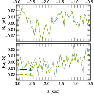
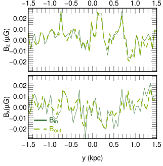
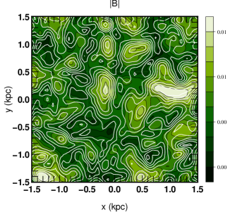
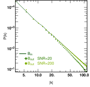
Figure 1: Top: input (solid lines) and recovered (dashed lines) $x$ and $z$ components of the field along a LOS (left) and along the $y$ transverse direction (right). The $y$ component and the $x$ direction are not plotted since very close to the $x$ component and the $y$ direction. One can see that the $z$ component is better reconstructed than the $x$ or $y$ components which is consistant with the variance measurements and the global conditioning of the problem (see section 3.3). The reconstruction is carried on a $N_{\mathbf{r}}=64$ grid with $N_{\nu}=64$ frequency channel. The data are generated linearly (see section 3) with a SNR$=20$. Bottom left: maps of $|B|$ for a transverse section after smoothing of the fields. The green images represents the input field while the superposed white contours show the recovered one. Bottom right: power spectra of the input field (solid line) and the recovered one (crosses). As expected, the recovered power spectrum is damped at higher frequencies because of the regularization. To illustrate this we added the power spectrum of a reconstruction with SNR=200.

2.3 Implementation

Given equations (18) and (19) the objective function writes:

$$\mathcal{Q}=(\mathbf{P}-\mathbf{d})^{\dagger}\cdot{\mathbf{C}}_{\mathrm{n}}^{-1}\cdot(\mathbf{P}-\mathbf{d})+\mu_{\mathrm{s}}\,\|\Delta^{{\alpha}/{4}}\mathbf{B}\|^{2}\,.$$ (22)

To minimize $\mathcal{Q}(\mathbf{B})$, we used a variable metric limited memory optimization method with BFGS updates (Nocedal, 1980) called VMLM and implemented in OptimPack (Thiébaut, 2002). Finding the optimal solution, equation (16), involves computing the gradient of equation (22) with respect to $\mathbf{B}$. Now differentiating equation (18) with respect to a magnetic field components we get

$$\frac{\partial\chi^{2}}{\partial\mathbf{B}_{i}}=2\,\mathcal{R}\mathrm{e}\left[(\mathbf{P}-\mathbf{d})^{\dagger}\cdot{\mathbf{C}}_{\mathrm{n}}^{-1}\cdot\frac{\partial\mathbf{P}}{\partial\mathbf{B}_{i}}\right]\,,$$ (23)

where ${\partial\mathbf{P}}/{\partial\mathbf{B}_{i}}$ for $i=x,y,z$ are given by equations (7) and (9). Similarly, differentiating equation (19) with respect to $\mathbf{B}$ yields

$$\frac{\partial\mathcal{R}}{\partial\mathbf{B}_{i}}=\mu_{\mathrm{s}}\,{\mathbf{F}}^{-1}\cdot\mathbf{\hat{B}}_{i}|\mathbf{k}|^{\alpha}\,.$$ (24)

The VMLM algorithm is a quasi-Newton method which proceeds by solving successive linear problems. Let us therefore first consider in the next section a linearized version of our inverse problem, which may correspond to a physically motivated problem when a good first guess for the magnetic field is known.

Note finally that equations (7) and (9) imply that ${\partial\chi^{2}}/{\partial\mathbf{B}_{i}}=\mathbf{0}$ at $B_{x}=B_{y}=0$. Note also that if $(B_{x},B_{y},B_{z})$ is a solution to equation (5), so is $(-B_{x},-B_{y},B_{z})$. Consequently we expect that the $\chi^{2}$ will be strongly multivalued as a function of $\mathbf{B}$. The smoothing penalty should in part prevent a pixel-by-pixel flip of the $x$ and $y$ component. It remains nonetheless to be shown that the zero divergence condition is sufficient to avoid flipping the field in regions bound by zeros of these two components, if such regions exist. Addressing these issues will be the topic of another paper.

3 Linearization

Let us first consider the situation when a fairly good guess for the overall magnetic field, $\mathbf{B}_{0}$, is known, on the basis, say of a first large scale investigation, or via some modelling of the field as a function of the underlying density (e.g. Cao et al., 2006; Kachelrieß et al., 2007). Let us then seek the departure from this guess. It is then legitimate to assume $\mathbf{B}=\mathbf{B}_{0}+\delta\mathbf{B}$, with, possibly (if the prime guess is accurate enough) $\delta\mathbf{B}/|\mathbf{B}_{0}|\ll 1$, so that equation (5) becomes:

$$\delta\mathbf{P}\equiv\left(\frac{\partial\mathbf{P}}{\partial\mathbf{B}}\right)_{\mathbf{B}_{0}}\cdot\,\delta\mathbf{B},$$ (25)

where the tensor $\partial\mathbf{P}/\partial\mathbf{B}_{i}$ is given by its components, equations (7), (8) and (9), while $\delta\mathbf{P}\equiv\mathbf{P}-\mathbf{P}(\mathbf{B}_{0})$. Now equation (25) is likely to be a much better behaved equation as the linearity warrants convexity of the objective function, hence the formal unicity of the solution.

In this paper, we will address two linear problems in turn, one of academic interest, to understand the properties of the inverse problem at hand, while the second one should allow us to carry realistic reconstructions, in the regime when a fair reference field is known. Specifically, we will first assume that the (noise free) data is in the image of $\left({\partial\mathbf{P}}/{\partial\mathbf{B}}\right)_{\mathbf{B}_{0}}$:

$$\mathbf{d}\equiv\delta\mathbf{P}_{L}=\left({\partial\mathbf{P}}/{\partial\mathbf{B}}\right)_{\mathbf{B}_{0}}\cdot\,\delta\mathbf{B}+\mathbf{e}\,,\quad\mbox{linear problem (I),}$$

while for the second problem (the so called Gauss-Newton approximation)

$$\mathbf{d}\equiv\delta\mathbf{P}_{\rm PL}\equiv\mathbf{P}-\mathbf{P}(\mathbf{B}_{0})+\mathbf{e}\,,\quad\mbox{pseudo linear problem (II).}$$

We investigate the linear problem in this section and the pseudo-linear problem in section 4.

3.1 Linear reconstruction

Let us illustrate our method on a problem of realistic scales. This first simulation is carried on a $N_{\mathbf{r}}^{3}$ grid ($N_{\mathbf{r}}=64$) with $N_{\nu}=64$ frequencies. The reference field $\mathbf{B}_{0}$ is chosen constant and set to $1\,\mu$G everywhere for each component, the power spectrum of the perturbation field $\delta\mathbf{B}$ has a power law index $\alpha=2$ and its RMS is $0.01$. Data are simulated linearly (see section 3) and are noised with a SNR$=20$. Figure 1 illustrates the quality of the reconstruction. The top panel represents the $x$ and $z$ components along the LOS ($z$ direction) or transverse ($y$ direction) for a given pixel. As the results for the $y$ component and the $x$ direction are similar to the $x$ component and the $y$ direction, they are not plotted. Here, the solid lines stand for the input field and the dashed lines for the recovered one. It is clear that the two fields are very similar and that the $z$ component is the best recovered (see section 3.3). The bottom left panel shows a map of $|B|$ for a transverse section after smoothing. The smoothing is made by convolving the field with a four pixels full-width at half maximum (FWHM) gaussian. The green features represent the input field and the reconstructed one is shown in the superposed white contours. The bottom right panel shows the power spectra of the input field (solid line) and the recovered one (crosses). Finally, figure 2 represents the field lines of the input field (top) and the recovered one (bottom). These figures show that, if the frequencies are correctly sampled (see section 3.2), the linear inverse problem (I) recovers qualitatively well the underlying field. The local and global properties of the field can be reconstructed provided that the linearization remains valid which will be investigated in section 4.

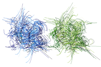
Figure 2: Field lines of the input (left) and the recovered (right) fields for a $64^{3}$ reconstruction with $N_{\nu}=64$ frequencies. The fields correspond to a reconstruction with a SNR of 200.

It is of interest to study the conditioning of the linear problem for two reasons (i) to understand the spatial spectral feature of the solution; in particular the biases of the eigenvectors of the linearized problem which induces anisotropy in the distribution of errors around the solution; (ii) to constrain the best sampling strategy in order to recover $\mathbf{B}$. Eventually it will also have an impact on our ability to carry out the non linear reconstruction.

The requirements to set up a good conditioning of the global inverse problem can be formulated in steps. First a necessary condition is to make a proper choice of the (electromagnetic) frequency sampling, which can be achieved by looking at a smaller subproblem on a given LOS; however, this optimal sampling does not warrant a good global conditioning; we therefore investigate the quality of the global linear reconstruction by looking at different elements of the reconstruction covariance matrix in (spatial) frequency space. In particular, we will show that the quality of the reconstruction is anisotropic and depends on the components of the field, $\mathbf{B}$, which is confirmed by looking at the eigenvectors of the covariance matrix for a low dimensional problem.

3.2 Conditioning of a line of sight and frequency sampling

One can see easily that in the relation between polarization and magnetic field (equation (5)), each line of sight is independent of the other. The link between them is provided by the solenoidal condition. In this subsection we will not consider this condition and the matrix $(\partial\mathbf{P}/\partial\mathbf{B})_{\mathbf{B}_{0}}$ becomes block-diagonal. Moreover, the three components can be separated leading to three different matrices, $(\partial\mathbf{P}/\partial\mathbf{B}_{x})$, $(\partial\mathbf{P}/\partial\mathbf{B}_{y})$ and $(\partial\mathbf{P}/\partial\mathbf{B}_{z})$. The field $\mathbf{B}_{0}$ is taken constant and its modulus set at $1\,\mu$G. In this case, all blocks are the same and the study of the conditioning is reduced to the study of three $N_{\nu}\times N_{\mathbf{r}}$ matrices with $N_{\nu}$ the number of frequencies and $N_{\mathbf{r}}$ the number of pixels in the $z$ direction.

Numerical investigations show that the conditioning of $(\partial\mathbf{P}/\partial\mathbf{B}_{x})$ depends mainly on the ratio $K\,h\,n_{\mathrm{e}}\,B_{z}/\nu^{2}$ leading to the conclusion that the conditioning is dominated by the exponential term of equation (7). It follows that $(\partial\mathbf{P}/\partial\mathbf{B}_{y})$ has the same behavior as $(\partial\mathbf{P}/\partial\mathbf{B}_{x})$ since the exponential terms are the same in both equations (7) and (8), which is confirmed numerically.

Recall that since in this section the reference field is chosen constant, so is $B_{z}$; therefore the best sampling for the frequencies is to have $\nu^{-2}_{n}-\nu^{-2}_{n+1}$ constant, that is a constant step for the squared wavelength; hence: $\lambda_{n}^{2}\equiv\lambda_{0}^{2}+(n-1)\,\Delta\lambda^{2}$ with $n=1,\ldots,N_{\nu}$ the index of the frequency/wavelength. So that the complex exponential becomes

$$\mathrm{e}^{2\,\mathrm{i}\,K\,n_{\mathrm{e}}\,B_{z}\,h\,m\,\lambda_{n}^{2}/c^{2}}$$

$$=\mathrm{e}^{2\,\mathrm{i}\,K\,n_{\mathrm{e}}\,B_{z}\,h\,m\,\lambda_{0}^{2}/c^{2}}\mathrm{e}^{2\,\mathrm{i}\,K\,n_{\mathrm{e}}\,B_{z}\,h\,m\,(n-1)\,\Delta\lambda^{2}/c^{2}}$$ (26)

with $m=1,\ldots,N_{\mathbf{r}}$ the pixel index along the line of sight. The value of $\Delta\lambda^{2}$ must be chosen in such a way that the frequency dependent complex exponentials are uniformly sampled on the complex circle. Hence $K\,n_{\mathrm{e}}\,B_{z}\,h\,N_{\mathbf{r}}\,(n-1)\,\Delta\lambda^{2}/c^{2}$ must be a multiple of $\pi$ for any $n$. With $L=h\,N_{\mathbf{r}}$ the maximum probed depth and taking the smallest multiple, this yields:

$$\Delta\lambda^{2}=\frac{\pi\,c^{2}}{K\,n_{\mathrm{e}}\,B_{z}\,L}\,.$$ (27)

With this particular choice, the matrices $(\partial\mathbf{P}/\partial\mathbf{B}_{x})$ and $(\partial\mathbf{P}/\partial\mathbf{B}_{y})$ take the following form:

$$(\partial\mathbf{P}/\partial\mathbf{B}_{x/y})_{n,m}=C_{x/y}e^{N_{\mathbf{r}}i\beta}\left(\lambda_{0}^{2}+\frac{(n-1)\pi}{K\,n_{\mathrm{e}}B_{z}L}\right)^{\frac{\gamma-1}{4}}$$

$$\times\left(e^{-i\beta}e^{\frac{-2i\pi(n-1)}{N_{\mathbf{r}}}}\right)^{N_{\mathbf{r}}-m},$$ (28)

where $\beta=2\,K\,n_{\mathrm{e}}\,B_{z}\,h\,\lambda_{0}^{2}$ and $C_{x/y}$ is a different constant in the $x$ and $y$ directions. If the factor $\left(\lambda_{0}^{2}+{(n-1)\pi}/({K\,n_{\mathrm{e}}B_{z}L})\right)^{\frac{\gamma-1}{4}}$ is set to 1, the matrix is a unitary Vandermond matrix and its conditioning is 1 (Cordova et al., 1990).

Accounting for this factor impairs the conditioning but it stays close to unity. The elements of the last matrix, $(\partial\mathbf{P}/\partial\mathbf{B}_{z})$ are just geometrical series of the elements of $(\partial\mathbf{P}/\partial\mathbf{B}_{x})$. Thus, they read:

$$\left({\partial\mathbf{P}}/{\partial\mathbf{B}_{z}}\right)_{n,m} = C_{z}e^{N_{\mathbf{r}}i\beta}\left(\lambda_{0}^{2}+\frac{(n-1)\pi}{K\,n_{\mathrm{e}}B_{z}L}\right)^{\frac{\gamma+3}{4}}\times$$

$$\hskip-85.35826pt\frac{\displaystyle 1-\exp({-i\beta(N_{\mathbf{r}}+1-m)})\exp\left({\frac{-2i\pi}{N_{\mathbf{r}}}(n-1)(N_{\mathbf{r}}+1-m)}\right)}{\displaystyle 1-\exp\left({-i\beta}\exp({-\frac{2i\pi}{N_{\mathbf{r}}}(n-1)})\right)}\,.$$

where $C_{z}$ is yet another constant. At this stage, there is only one free parameter left, the first frequency $\lambda_{0}$. The conditioning of $\left({\partial\mathbf{P}}/{\partial\mathbf{B}_{x/y}}\right)$ being always close to unity, the value of $\lambda_{0}$ must be chosen in order to minimize the conditioning of $\left({\partial\mathbf{P}}/{\partial\mathbf{B}_{z}}\right)$.

Figure 3 (top panel) represents the conditioning of $\left({\partial\mathbf{P}}/{\partial\mathbf{B}_{z}}\right)$ as a function of $\lambda_{0}$ for different grid sizes. The curves are very similar in shape and the best conditioning is represented by the red dots. In the bottom panel the wavelength providing the best conditioning for $\left({\partial\mathbf{P}}/{\partial\mathbf{B}_{z}}\right)$ is plotted as a function of the grid size. It appears that $\lambda_{0}\propto\sqrt{N_{\mathbf{r}}}$ and the precision on $\lambda_{0}$ is not really important since the minimum of the curves are not really marked. These particular choices of $\lambda_{0}$ give a conditioning of $1.29$ for $\left({\partial\mathbf{P}}/{\partial\mathbf{B}_{x/y}}\right)$, whatever grid size.

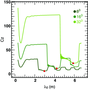
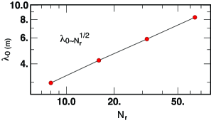
Figure 3: Top: conditioning, $C_{z}$, of $\left({\partial\mathbf{P}}/{\partial\mathbf{B}_{z}}\right)$ as a function of $\lambda_{0}$ for different grid sizes. The red dots represent the best conditionings. Bottom: $\lambda_{0}$ giving the best conditioning as a function of the grid size, $N_{\mathbf{r}}$. It appears that $\lambda_{0}\propto\sqrt{N_{\mathbf{r}}}$.

3.3 Conditioning of ${\mathbf{C}}_{\mathrm{MAP}}$ and a posteriori variances

Let us now investigate the a posteriori variances of different spatial frequencies of the reconstructed field. This covariance matrix can be written as

$${\mathbf{C}}_{\mathrm{MAP}}=({\mathbf{A}}^{T}\cdot{\mathbf{C}}_{\mathrm{n}}^{-1}\cdot{\mathbf{A}}+{\mathbf{C}}_{\mathbf{B}}^{-1})^{-1},$$ (29)

where ${\mathbf{A}}\equiv\left({\partial\mathbf{P}}/{\partial\mathbf{B}_{0}}\right)\cdot{\mathbf{\Pi}}$ with ${\mathbf{\Pi}}$ the projector that cancels the divergence (cf. equation (20)) and ${\mathbf{C}}_{\mathrm{n}}^{-1}$ and ${\mathbf{C}}_{\mathbf{B}}^{-1}\equiv\mu_{\mathrm{s}}\,\mathbf{F}^{-1}{\rm diag}(|k|^{\alpha})\mathbf{F}$ are the a priori covariance matrices of the noise and the signal respectively. Here we seek $\hat{{\mathbf{C}}}_{\mathrm{MAP}}$, the Fourier transform of ${\mathbf{C}}_{\mathrm{MAP}}$ as we want to understand the relative error in the amplitude of the spatial modes of $\mathbf{B}$. Because of the potential high dimensionality of our problem, the covariance matrix, $\hat{{\mathbf{C}}}_{\mathrm{MAP}}$ is not computed directly. We chose instead to compute the selected values by solving for $\mathbf{\hat{B}}$ the following equation with a conjugate gradient method (CGM, Shewchuk, 1994; Nocedal & Wright, 2006):

$$\hat{{\mathbf{W}}}_{\mathrm{MAP}}\cdot\hat{\mathbf{B}}=\hat{\mathbf{B}}_{\rm ref}.$$ (30)

Here, $\hat{{\mathbf{W}}}_{\mathrm{MAP}}=\hat{{\mathbf{C}}}_{\mathrm{MAP}}^{-1}$ and the solution, $\hat{\mathbf{B}}$, found by the CGM is

$$\hat{\mathbf{B}}=\hat{{\mathbf{C}}}_{\mathrm{MAP}}\cdot\hat{\mathbf{B}}_{\rm ref}.$$ (31)

The reference field, $\hat{\mathbf{B}}_{\rm ref}$, is equal to $1$ or $\pm i$ for the chosen $\mathbf{k}$ frequency and its opposite $-\mathbf{k}$ in order to have a real field, and $0$ elsewhere. The elements $\hat{\mathbf{B}}_{\mathbf{k}}$ and $\hat{\mathbf{B}}_{-\mathbf{k}}$ of the solution are combinations of the covariance of $\mathbf{k}$ and $-\mathbf{k}$ and the variance of $\mathbf{k}$. It allows us to determine the a posteriori variance of the chosen spatial frequency $\mathbf{k}$. To check this method, the same variances were also computed by the iterative VMLM method. One can check that:

$$\langle(\hat{\mathbf{B}}_{\rm in}-\hat{\mathbf{B}}_{\rm out})\cdot(\hat{\mathbf{B}}_{\rm in}-\hat{\mathbf{B}}_{\rm out})^{\dagger}\rangle=\hat{{\mathbf{C}}}_{\mathrm{MAP}},$$ (32)

where $\dagger$ denotes conjugate transposition, $\hat{\mathbf{B}}_{\rm in}$ and $\hat{\mathbf{B}}_{\rm out}$ stand respectively for the input field and the reconstructed one in Fourier space. As expected, the higher the number of iterations, the closer the two estimates of the variance.
Figure 4 represent the evolution of the a posteriori variance of different spatial frequencies $\mathbf{k}$ for the different components of the field in different directions (along a LOS or transverse to it) as a function of the SNR. The size of the box is $N_{\mathbf{r}}=16$ and the number of frequencies is $N_{\nu}=16$. Figure 5 shows the evolution of the a posteriori variances of the same frequencies as of figure 4, but as a function of the spectral index, $\alpha$, of the sought field (for a SNR$=20$). As expected, the variance decreases as the index increases.

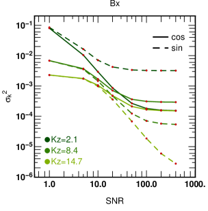
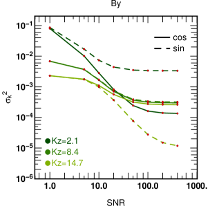
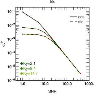
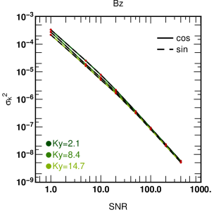
Figure 4: A posteriori variance of different spatial frequencies $\mathbf{k}\in(1,2,3)$ for the different components of the field in different directions (along a LOS or transverse to it) as a function of the SNR. The size of the box is $N_{\mathbf{r}}=16$ and the number of frequency is $N_{\nu}=16$. The top panels correspond to the variation of $\sigma_{k}^{2}$ for three different values of $k_{z}$ while the bottom panels correspond to varying $k_{y}$. The cosine mode (thick line) and sine mode (dashed line) are both shown. All variances decrease with increasing SNR as expected, although at different rate, see the main text. Note the different amplitude in $\sigma^{2}_{k}$ for the bottom right panel which shows that the $\mathbf{B}_{z}$ component of the field is better recovered compared to the other components. This reflects the anisotropy of the model $\mathbf{A}$ which induces anisotropic reconstruction errors.

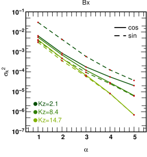
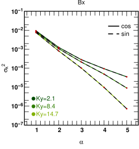
Figure 5: Same as Figure 4 but as a function of the spectral index, $\alpha$, of $\delta\mathbf{B}$ for a SNR$=20$. As expected, the smoother the expected field, the larger $\alpha$, the smaller the posterior variances.

In Figure 4 the SNR is defined as

$${\rm SNR}={\rm RMS(data)}/\sigma_{\mathrm{n}},$$ (33)

with $\sigma_{\mathrm{n}}^{2}$ standing for the noise variance. The results for the $B_{y}$ and $B_{z}$ fields in the $x$ direction are not plotted because there are exactly the same as those in the $y$ direction. First note that the variances, $\sigma^{2}_{k}$ for the $\mathbf{B}_{z}$ component of the field are much smaller in amplitude relative to the other components. For the $\mathbf{B}_{x}$ and $\mathbf{B}_{y}$ fields, at low SNR, the Wiener prior is important in the reconstruction, explaining the separation of the three curves corresponding to three different scales. In Fourier space, $\hat{{\mathbf{C}}}_{\mathbf{B}}=\mu_{\mathrm{s}}^{-1}\,{\rm diag}(|k|^{-\alpha})$ with $\alpha$ the spectral index of the power spectrum of the input field. If the regularization dominates, $\hat{{\mathbf{C}}}_{\mathrm{MAP}}\sim|k|^{-\alpha}$, which corresponds to the values on the figures when the SNR is low.

For the transverse frequencies (bottom panels), the behaviour of the variances is well understood. At low SNR, the Wiener prior dominates the reconstruction for the $\mathbf{B}_{x}$ and $\mathbf{B}_{y}$ components but not for the $\mathbf{B}_{z}$ one. Increasing the SNR implies increasing the relative weight of the data compared to the prior. So equation (29) becomes

$${\mathbf{C}}_{\mathrm{MAP}}\sim({\mathbf{A}}^{T}\cdot{\mathbf{C}}_{\mathrm{n}}^{-1}\cdot{\mathbf{A}})^{-1},\quad\mbox{when SNR }\rightarrow\infty\,.$$ (34)

If we assume a Gaussian white noise, ${\mathbf{C}}_{\mathrm{n}}=\sigma_{\mathrm{n}}^{2}\,{\mathbf{I}}$ with ${\mathbf{I}}$ the identity matrix, equation (34) becomes

$${\mathbf{C}}_{\mathrm{MAP}}\sim\sigma_{\mathrm{n}}^{2}({\mathbf{A}}^{T}\cdot{\mathbf{A}})^{-1}\,,$$ (35)

so ${\mathbf{C}}_{\mathrm{MAP}}\propto\sigma_{\mathrm{n}}^{2}$ or given equation (33), ${\mathbf{C}}_{\mathrm{MAP}}\propto{\rm SNR}^{-2}$ which is the slope of these curves. Finally, note that there is no symmetry breaking between the $x$ and $y$ directions and between the $x$ and $y$ components of the field or between the sine and cosine modes in ${\mathbf{C}}_{\mathrm{MAP}}$.
Now, consider the $x$ and $y$ components of the field along a LOS (top panels). At low SNR, the Wiener prior still dominate, providing the same value as in the transverse direction. Then, the variance decreases as SNR^-2 but reaches a threshold and stagnate. It is clear on the figures that there is a symmetry breaking between the $x$ and the $y$ components of the field and a separation between the sine and cosine modes. At first it may be surprising that the variances reach a threshold since the frequencies have been chosen to provide the best possible conditioning for $\left({\partial\mathbf{P}}/{\partial\mathbf{B}_{0}}\right)$ along a LOS (see section 3.2). In fact this is a consequence of the solenoidal condition. Recall that for the global inverse problem, the relevant linear model is ${\mathbf{A}}=\left({\partial\mathbf{P}}/{\partial\mathbf{B}_{0}}\right)\cdot{\mathbf{\Pi}}$, where ${\mathbf{\Pi}}$ is the projector given by equation (20). This projector changes the matrix $\left({\partial\mathbf{P}}/{\partial\mathbf{B}_{0}}\right)$ and adds off-diagonal terms to the block diagonal matrix considered in the previous subsection. In effect, the solenoidal condition degrades the global conditioning relative to the one LOS problem (but recall that without it we have an ill posed problem). In turn this changes the eigen structure of $\hat{{\mathbf{C}}}_{\mathrm{MAP}}$ and therefore its projection in Fourier space.

Indeed, let us compute directly the whole matrix $\hat{{\mathbf{C}}}_{\mathrm{MAP}}$ for a smaller, more tractable $N_{\mathbf{r}}=8$ constant reference magnetic field with $N_{\nu}=8$ frequencies sampled following the procedure defined in section 3.2. Figure 6 shows the global conditioning of the covariance matrix ${\mathbf{C}}_{\mathrm{MAP}}$ as a function of the SNR. One can see that the mixing of the LOS has a significant effect on conditioning, even though the frequencies were chosen optimally. Figure 6 also shows that at realistic SNR, the global conditioning remains bounded and could be improved, e.g. for the purpose of numerical convergence, by artificially increasing the hyperparameter $\mu_{\mathrm{s}}$. Note finally that even though the global conditioning increases with the SNR, the variances all decrease, as expected.

3.4 Eigenspace analysis

In order to understand the plateau on figure 4, let us also explicitly diagonalize ${\mathbf{W}}_{\mathrm{MAP}}$ for the smaller above-described $N_{\mathbf{r}}=8$ problem with a SNR$=20$. The corresponding spectrum is plotted on figure 7, bottom right panel. The global conditioning of ${\mathbf{W}}_{\mathrm{MAP}}$ is about $10^{5}$ (consistently with what was shown on Figure 6 for ${\mathbf{C}}_{\mathrm{MAP}}$), but note importantly that there is a cluster of eigenvalues followed by a gap. This gap is consistent with the plateau seen on figure 4. When increasing the SNR, one expects to filter out less and less eigen modes, and therefore to access more and more eigenvectors (corresponding to decreasing eigenvalues) in the reconstruction. However, when reaching the gap, although the SNR increases, no more eigenvalues are available for a while. The lower eigenvectors, encoding informations on higher frequencies, are not within reach, and the a posteriori variance of these frequencies stagnate, as seen in figure 4. If the SNR increases further, these eigenvalues (and therefore their associated eigenvectors) will be sampled, and we expect that the $\sigma^{2}_{k}$ variances will decrease again. The modulus of the first eigenvector (associated to the highest eigenvalue) is plotted on the top panels in the $x\!-\!y$ (left) and $x\!-\!z$ (right) planes. It is clear on these figures than the $x$ and $y$ directions are isotropic while the $z$ one is anisotropic for this eigenvector. Moreover, the component of the power spectra in the bottom left panel show that the $B_{z}$ component clearly differ from the other two components.

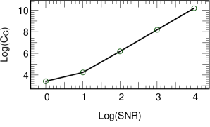
Figure 6: Global conditioning of the (a posteriori) covariance matrix ${\mathbf{C}}_{\mathrm{MAP}}$ as a function of the SNR. The higher the signal to noise, to more difficult the inversion, but the smaller the covariance a posteriori. The 3D matrix, ${\mathbf{A}}=\left({\partial\mathbf{P}}/{\partial\mathbf{B}_{0}}\right)\cdot{\mathbf{\Pi}}$ appears to be more poorly conditioned than its 1D counterpart even though the sampling in electromagnetic frequency was the same as in section 3.2. It remains bounded and within reach of double precision calculation.

However, all of the main eigenvectors do not behave in the same way. Some of them clearly break the symmetry between the $x$ and $y$ directions or/and between the $x$ and $y$ components leading to the differences in the curves of figure 4. Finally note that the main eigenvectors are fairly high frequencies fields. So, the a posteriori variances will be smaller for high frequencies than for low ones, which is reflected by the top panels of figure 4.

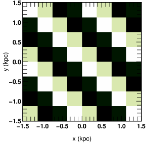
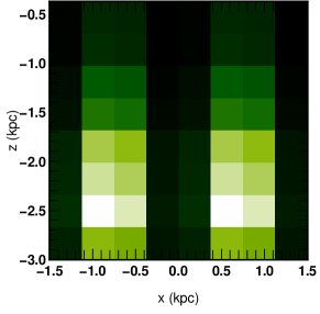
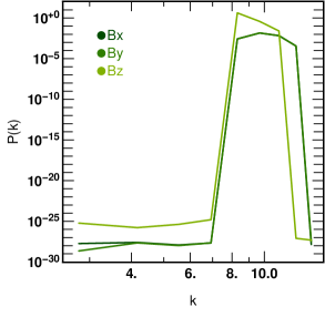
Figure 7: Top panels: maps of the modulus of the field corresponding to the first eigenvector of ${\mathbf{W}}_{\mathrm{MAP}}$ in the $x\!-\!y$ (left) and $x\!-\!z$ (right) plans for a $8^{3}$ constant reference magnetic field with $N_{\nu}=8$ frequencies sampled as explained in section 3.2 with a SNR$=20$. The first eigenvector appears to be isotropic in $x$ and $y$ and anisotropic in the $z$ direction. Bottom left: power spectra of the three components of this eigenvector. The anisotropy of the $z$ component is clearly visible and in good agreement with the results found in section 3.1 (figure 1) and 3.3 (figure 4). Bottom right: spectrum of the eigenvalues of ${\mathbf{W}}_{\mathrm{MAP}}$.

4 Validity of the linear approximation

4.1 Linear and pseudo linear inversion

Let us first carry out a linear inversion of the same pertubative field $\delta\mathbf{B}$, with RMS$(\delta\mathbf{B})=10^{-3}\mu$G, while considering both the linear (I) and the pseudo linear (II) data sets (see section 3). We work here on a $N_{\mathbf{r}}=64$ grid, with $N_{\nu}=64$ frequencies, a constant reference field of module 1 $\mu$G and SNR=$20$. Recall that for the linear minimum variance solution, the hyperparameter $\mu_{\mathrm{s}}=1/{\rm P}(k=1)$ (see section 2.2.2), while for the the pseudo linear data set it may be tuned. Figure 8 top panel shows the input $z$ component for the input field (solid line) along a given LOS and the output ones (dotted line for the linear data, $\delta\mathbf{P}_{L}$ and dashed line for the pseudo linear, $\delta\mathbf{P}_{\rm PL}$) while the bottom panel shows the different power spectra. As previously, the field recovered from linearized data sets fits quite well the input one. The recovered pseudo linear field, though somewhat different from the linear one, remains fairly close to the original field. The corresponding powers pectra are also shown on Figure 8 and confirm that the recovered field in setting (II) is quantitatively redder.

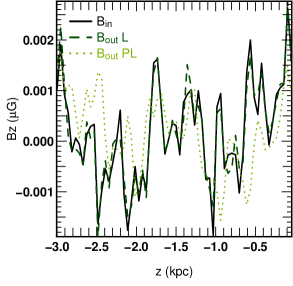
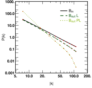
Figure 8: Top: $\mathbf{B}_{z}$ along a LOS for the input field (solid line) and for the recovered fields with linear data, $\delta\mathbf{P}_{L}$ (dashed line) and pseudo linear ones, $\delta\mathbf{P}_{\rm PL}$ (dotted line) (see section 3). Bottom: power spectra of these three fields. Note that the power spectrum of the reconstructed field from the pseudo linear data set is steeper.

4.2 Second order residuals

Let us now study the second order residuals to quantify the domain of validity of the linearization. For this purpose, we subtract to the total polarization its zero and first order expansion to obtain ($\mathbf{P}-\mathbf{P}_{0}-\left({\partial\mathbf{P}}/{\partial\mathbf{B}}\right)_{\mathbf{B}_{0}}\propto\delta\mathbf{B}^{2}$) and we divide this quantity by the first order term ($\mathbf{P}-\mathbf{P}_{0}\propto\delta\mathbf{B}$). Figure 9 represents the average of this quantity as a function of RMS$(\delta\mathbf{B})$. Here the perturbation consist of a single frequency and single component field. The solid lines represent the results obtained with a $B_{x}$ component along the LOS at the lowest mode, while the dashed lines correspond to the lowest transverse mode of the $B_{z}$ component. The dark curves represent the real part, $Q$, of the polarization while light ones stand for the imaginary part $U$ (see equation (1)). At very low RMS$(\delta\mathbf{B})$, numerical noise dominate but decreases as the RMS increases. After reaching a minimum, note that the quantity plotted increase as RMS$(\delta\mathbf{B})$ since $\propto\delta\mathbf{B}^{2}/\delta\mathbf{B}$ and thus $\propto\delta\mathbf{B}$. As expected, the lower the RMS$(\delta\mathbf{B})$, the better the linear approximation and the better the reconstruction. Note also the significant amplitude difference between the $\mathbf{B}_{z}$ and $\mathbf{B}_{x}$ components; we interpret this as a difference between the second derivatives of the field, which in turn, impairs the accuracy of the linearization for the $z$ component. This should not be a limitation when carrying the non linear reconstruction using a method such as VMLM, as the amplitude of the subsequent changes in the magnetic field will be scaled by the inverse second derivatives.

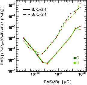
Figure 9: Average second order of the polarization divided by the first order as a function of RMS$(\delta\mathbf{B})$. Here RMS$(\delta\mathbf{B})$ is a single component and single mode field. Results are for a the lowest longitudinal mode for the $x$ component (solid lines) and the lowest transverse mode for the $z$ component (dashed lines). Dark curves represent the real part $Q$ of the polarization while light ones are for the imaginary part $U$ (see equation (1)).

4.3 Towards the non linear problem

Up to now, we have only considered the situation where $\mathbf{B}_{0}$ was assumed to be constant. What happens to the conditioning when we add spatial frequencies to $\mathbf{B}_{0}$ or/and over $\,n_{\mathrm{e}}$? It is easy to see that adding transverse frequencies to the $x$ or the $y$ component of $B$ will not change the conditioning of a LOS. Indeed, according to equations (7) and (28), only the constants $C_{x/y}$ are modified and vary for each LOS, but remain constant along each of them, which has no effect on conditioning. On the contrary, if the modulation is along a LOS, $C_{x/y}$ is no longer constant, and varies for every pixel along a LOS. However, given that the conditioning is dominated by the exponential terms in the Vandermond approximation, it doesn’t change dramatically. Hence the choice of $\lambda_{0}$ and the sampling frequency remain the same but the conditioning increases slightly; it can reach $3$ for $\left({\partial\mathbf{P}}/{\partial\mathbf{B}_{x/y}}\right)$ and $40$ for $\left({\partial\mathbf{P}}/{\partial\mathbf{B}_{z}}\right)$.
The situation is a priori more dramatic for the $z$ component of the field or for the electronic density $\,n_{\mathrm{e}}$. Indeed, the addition of a transverse modulation has significant consequences, as the value of $B_{z}$ (or/and $\,n_{\mathrm{e}}$) in equation (27) becomes different for each LOS. Therefore, the value of $\Delta\lambda^{2}$ should in principle be different for each LOS to conserve the best conditioning. In practice it is simplest to take the average of $\mathbf{B}_{z}$ (or/and $\,n_{\mathrm{e}}$) as a guess. However the conditioning per LOS increases signicantly and the quality of the reconstruction should be affected.
However, it appears that the global conditioning of ${\mathbf{C}}_{\mathrm{MAP}}$ does not change dramatically compared to the constant reference field value, whatever the frequency and the amplitude of the added modulation. The solenoidal condition appears to be very effective. In fact, the repetition of the spectral analysis carried in section 3.4, shows that the main difference will be in the gap seen on figure 7. Adding modulation on a constant field induces earlier, deeper gaps. At fixed SNR, the number of useful eigenvalues for the reconstruction decreases with the modulation. The inversion can still be carried, but will be more biased by the lack of resolved eigenmodes.

As a final illustration, figure 10 shows an implementation of the linear inversion on a more realistic reference field, $\mathbf{B}_{0}$ which is extracted from a magneto-hydrodynamical simulation (Kowal & Lazarian, 2007), perturbed by a power-law fluctuation with a power spectrum of $\alpha=2$ and a relative amplitude of $10^{-2}$ from a virtual data set of SNR=20. Note that for this more realistic illustration the electronic density $\,n_{\mathrm{e}}$ is not constant but extracted from the same simulation. Both the shape of the correction and its power-spectrum are well recovered for this relative amplitude reflecting that although non constant model and electronic density impair the conditionning, reconstructions remain possible.

5 Conclusion and perspectives

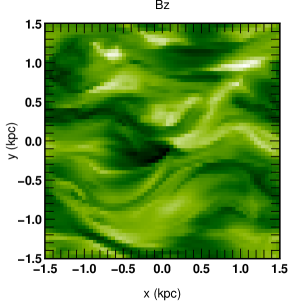
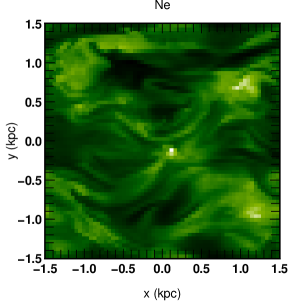
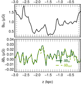
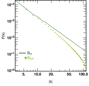
Figure 10: left top panel: map of a slice (of width $0.047$kpc) of input reference magnetic field, $\mathbf{B}_{0}$; right top panel: map of the same slice but for the known electronic density $\,n_{\mathrm{e}}$; left bottom panel: the input reference magnetic field, the input perturbation and the recovered one along a LOS. The perturbation field is a power-law fluctuation with a power spectrum of $\alpha=2$ and a relative amplitude of $10^{-2}$ from a virtual data set of SNR=20; right bottom panel: input and recovered power spectra of the perturbation field.

We investigated the problem of reconstructing the three-dimensional spatial structure of the magnetic field of a given simulated patch of our Galaxy, using multi-frequency polarized maps of the synchrotron emission at radio wavelengths.
When starting from a fair approximation of the magnetic field, we were able to obtain a good estimate of the underlying field by using a linearized version of the inverse problem considered, up to a $64^{3}$ grid size. The spectral analysis of the strictly linear problem (with a constant reference field, and the simulated data obtained through a linearized model) allowed us to specify the best sampling strategy in electromagnetic frequency, and predict a spatially anisotropic distribution of posterior errors.
The best sampling strategy is in equal $\Delta\lambda^{2}$; it follows from the shape of $\left({\partial\mathbf{P}}/{\partial\mathbf{B}_{0}}\right)$ along one LOS, which can be approximately recast into a unitary Vandermond matrix when this particular sampling is used. The errors on the reconstructed $B_{x}$ and $B_{y}$ components of the field are shown to be larger than the error on the $B_{z}$ component. This anisotropy can be traced back to the shape of the posterior covariance, and ultimately of the linearized model which is highly anisotropic, as only the $z$ component of the field induces Faraday rotation.

We considered in turn three more realistic cases: (i) a pseudo linear model (linear reconstruction of non-linearly simulated data), (ii) a varying reference model $\mathbf{B}_{0}$, and (iii) a varying reference model $\mathbf{B}_{0}$ and a (known) varying electronic density $\,n_{\mathrm{e}}$. We found that for these reconstructions, the global conditioning of the minimum variance solution remained tractable. Finally, we investigated the case where the reference field is given by the outcome of a magneto-hydrodynamical simulation, and is perturbed by an additional fluctuating component of known power spectrum. We showed that even in this case the linear reconstruction quality is reasonable. This leads us to claim that a full non-linear reconstruction, based on a Gauss-Newton sequence of linear sub-problems of varying reference field, should be achievable.

Possible extensions of this work, beyond the scope of this paper, involve investigating systematically the degeneracies of the non-linear inversion. It would be worthwhile to construct specific estimators for the (possibly anisotropic) local power spectrum of the field (see e.g. Lazarian & Pogosyan, 2006). Finally, from a modelling point of view, one of the main limitations of the present method is that we had to assume known thermal and relativistic electronic densities, in order to obtain a well posed inverse problem from synchrotron emission data alone. However, we could in principle relax this assumption by adding extra data constraining the electronic densities (e.g. H_α data, see Haffner et al., 2003) or emission measures of pulsars, and attempt a joint reconstruction of the magnetic field and the electronic densities. Any prior statistical information (e.g. extracted from MHD simulations) of possible correlation between $\mathbf{B}$ and $n_{\mathrm{e}}$ could be used in this context. Another possibility would be to use the extra information given by the circular polarization of synchrotron emission (see Appendix C); this circular polarization, if negligible in the case of low energy sources (like our Galaxy), is measurable in the case of relativistic radio sources (see e.g. Jones & Odell, 1977), and opens a way to constrain the electronic density together with the magnetic field structure of the source.

Acknowledgments

We thank Jean Heyvaerts, Martin Lemoine and Guy Pelletier for fruitful comments on the early stages of this work. Special thanks to Alex Lazarian for providing us with his interstellar magneto hydrodynamics simulations.

Appendix A The case $\gamma=3$

For $\gamma=3$, equation (5) takes a particularly simple expression

$$P=A\int_{-\infty}^{0}\nu^{-1}\,n_{\mathrm{r}}(z)(B_{x}^{2}(z)-B_{y}^{2}(z)+2iB_{x}(z)B_{y}(z))$$

$$\times\exp\left(\frac{2iK}{\nu^{2}}\int_{z}^{0}(\,n_{\mathrm{e}}B_{z})(z^{\prime\prime})dz^{\prime\prime}\right){{\mathrm{d}}}z\,,$$ (36)

while equation (8) simplifies to:

$$\frac{\partial P(\mathbf{x}_{\perp},\nu)}{\partial B_{x}({\bf\mathbf{r}^{\prime}})} = \delta_{\rm D}(\mathbf{r}-{\bf\mathbf{r}^{\prime}})2Ah\nu^{-1}\,n_{\mathrm{r}}({\bf\mathbf{r}}^{\prime})(B_{x}+iB_{y})({\bf\mathbf{r}}^{\prime})$$ (37)

$$\hskip-42.67912pt\times\exp\left(\frac{2iKh}{\nu^{2}}\sum_{z^{\prime\prime}}\theta_{\rm H}(z^{\prime\prime}-z^{\prime})(\,n_{\mathrm{e}}B_{z})(x^{\prime},y^{\prime},z^{\prime\prime})\right)\,.$$

Note that for this value of $\gamma$ the two derivatives with respect to the transverse magnetic field are thus related:

$$\frac{\partial P(\mathbf{x}_{\perp},\nu)}{\partial B_{y}({\bf\mathbf{r}^{\prime}})}=i\frac{\partial P(\mathbf{x}_{\perp},\nu)}{\partial B_{x}({\bf\mathbf{r}^{\prime}})}\,.$$ (38)

Appendix B Solenoidal fields with fixed power spectrum.

The generation of solenoidal (divergence free) fields with fixed power spectra up to the Nyquist frequency is a tricky problem. The field must obey the three following conditions:

1. fixed power spectrum: $P(\mathbf{k})\propto\mathbf{k}^{-\alpha}$,

2. free divergence: $\mathbf{\nabla}\cdot B\equiv 0\Leftrightarrow\bf{k}\cdot\hat{B}\equiv 0$,

3. reality of the field: $\hat{B}_{\mathbf{k}}=\hat{B}_{-\mathbf{k}^{\star}}$.

Given conditions (i) and (ii), the field is best generated in Fourier space. Since the field is multi periodic and we may write

$$\hat{B}=\hat{B}_{\perp 1}\mathbf{e}_{\perp 1}+\hat{B}_{\perp 2}\mathbf{e}_{\perp 2}\,,$$ (39)

where $\mathbf{e}_{\parallel}\equiv\mathbf{k}/|\mathbf{k}|$, $\mathbf{e}_{\perp 1}\>{\rm and}\,\mathbf{e}_{\perp 2}$ form a spherical basis in Fourier space, while $\hat{B}_{\perp,i}$, i=1,2 are the projection over that basis of the Fourier componant of the field. The vectors $\mathbf{e}_{\perp 1}\>{\rm and}\,\mathbf{e}_{\perp 2}$ are chosen in such a way that $\mathbf{e}_{\mathbf{k}\perp 1/2}=-\mathbf{e}_{-\mathbf{k}\perp 1/2}$. The spherical basis is direct for $\mathbf{k}$ and indirect for $-\mathbf{k}$. In this representation, conditions (ii) and (iii) become,

$$\hat{B}_{\mathbf{k}\perp 1/2}=-\hat{B}_{-\mathbf{k}\perp 1/2}^{\star},\quad{\rm and}\quad\hat{B}_{\mathbf{k}\parallel}=0.$$ (40)

So, the first step is to generate two complex fields $\hat{B}_{\perp 1}$ and $\hat{B}_{\perp 2}$ with the sought power spectrum and then apply equation (40).
Next, consider the frequencies that have no conjugate, i.e. the frequency $k_{i}=0$ (constant) and $k_{i}=N_{y}$ (Nyquist frequency) where the index $i$ represents the Cartesian coordinates. Let us define $F_{1}$ as the set of these two particular values, i.e. $F_{1}=[0,N_{y}]$, and $F_{2}$ the set of all the other values, i.e. for a vector of dimension $N$, $F_{2}=[-(N/2-1),-(N/2-2),...,-1,1,...N/2-2,N/2-1]$. When the three components of $\mathbf{k}$ belong to $F_{1}$, the reality condition of the field is merely $\mathcal{I}\mathrm{m}\hat{B}=0$. After putting this imaginary part to $0$, the field can be projected into the Cartesian basis.
The difficulty arises when one or two components belong to $F_{1}$. For example, consider the frequency $\mathbf{k}=(k_{x},k_{y},k_{z})$ with $k_{x}\in F_{1}$, $k_{y}$ and $k_{z}\in F_{2}$. In this case, condition (iii) become $\hat{B}_{\mathbf{k}}=\hat{B}_{-\tilde{\mathbf{k}}^{\star}}$ where $\tilde{\mathbf{k}}=(k_{x},-k_{y},-k_{z})$ is the “opposite” of $\mathbf{k}$. The problem is that in this case, $\mathbf{e}_{\mathbf{k}\perp 1/2}\neq-\mathbf{e}_{-\tilde{\mathbf{k}}\perp 1/2}$ and the above discussed method can no longer apply. Fortunately, the combination of condition (ii) and $\hat{B}_{\mathbf{k}}=\hat{B}_{-\tilde{\mathbf{k}}^{\star}}$ leads to the following set:

$$\bf{k}\cdot\hat{B}\equiv 0,\quad{\rm and}\quad\hat{B}_{\mathbf{k}_{x}}=0.$$ (41)

So, the trick is to put the faulty component to $0$ and to generate the other two as previously but in 2D space. Now, if $\mathbf{k}_{{\rm 2D}}=(k_{y},k_{z})$, we generate $\hat{B}=\hat{B}_{\perp{\rm 2D}}\mathbf{e}_{\perp\rm 2D}$, where $\mathbf{e}_{\parallel\rm 2D}\equiv\mathbf{k}_{\rm 2D}/|\mathbf{k}_{\rm 2D}|$ and $\mathbf{e}_{\perp\rm 2D}$ form a polar basis in Fourier space. As previously, the vectors $\mathbf{e}_{\perp\rm 2D}$ are chosen in such a way that $\mathbf{e}_{\mathbf{k}_{\rm 2D}\perp\rm 2D}=-\mathbf{e}_{-\mathbf{k_{\rm 2D}}\perp\rm 2D}$. In this 2D representation, conditions (ii) and (iii) lead to:

$$\hat{B}_{\mathbf{k}_{\rm 2D}\perp\rm 2D}=-\hat{B}_{-\mathbf{k}_{\rm 2D}\perp\rm 2D}^{\star},\\ \quad{\rm and}\quad\hat{B}_{\mathbf{k}_{\rm 2D}\parallel\rm 2D}=0.$$ (42)

Here we have only one degree of freedom left, thus, for these frequencies, we must generate one complex field $\hat{B}_{\perp\rm 2D}$ with the desired power spectrum, and then apply equation (42). When $k_{y}$ or $k_{z}$ belongs to $F_{1}$, a similar procedure applies.
In the last case, two component belong to $F_{1}$. For example, $\mathbf{k}=(k_{x},k_{y},k_{z})$ with $k_{x}\in F_{2}$, $k_{y}$ and $k_{z}\in F_{1}$. In this case, condition (iii) become $\hat{B}_{\mathbf{k}}=\hat{B}_{-\tilde{\mathbf{k}}^{\star}}$ where $\tilde{\mathbf{k}}=(-k_{x},k_{y},k_{z})$ is the “opposite” of $\mathbf{k}$. Again, $\mathbf{e}_{\mathbf{k}\perp 1/2}\neq-\mathbf{e}_{-\tilde{\mathbf{k}}\perp 1/2}$ and the combination of condition (ii) and $\hat{B}_{\mathbf{k}}=\hat{B}_{-\tilde{\mathbf{k}}^{\star}}$ leads to equations (41). Consequently, the same procedure follows for these frequencies. After inverse Fourier transform, one can check that the field is real, solenoidal and with the right power spectrum up to the Nyquist frequency.

Appendix C Circular Polarization

Since the rotating term depends on the density field of thermal electrons $n_{\mathrm{e}}$ in the medium, we cannot separate, with the Faraday rotation only, $n_{\mathrm{e}}$ from $B_{z}$. One way to tackle this problem is to pick up the next coupling term of the Stokes parameters in the (optically thin medium, strong rotativity limit) assumption that describes our medium. This next term is a factor of conversion between linear and circular polarization, that can be considered together with the synchrotron emissivity of circular polarization (Jones & Odell, 1977). Following the notations of Sazonov (1969), we write the transfer equation of the polarization tensor $I_{\alpha\beta}$ as follows:

$$\frac{\ {{\mathrm{d}}}I_{\alpha\beta}(z)}{{{\mathrm{d}}}z}=E_{\alpha\beta}(z)-i(T_{\alpha\sigma}(z)\delta_{\beta\tau}-\delta_{\alpha\sigma}T_{\beta\tau}^{*}(z))I_{\sigma\tau}(z)\,,$$ (43)

with $I_{\alpha\beta}=\left(\begin{array}[]{cc}I+Q&U+iV\\ U-iV&I-Q\end{array}\right)$, and $E_{\alpha\beta}(z)$ is an emissivity term. In the assumption of a thin, strongly rotating medium, we can retain only the rotating terms (the Hermitian part) of $T_{\alpha\beta}$. Defining $T=\left(\begin{array}[]{cc}h&q+if\\ q-if&-h\end{array}\right)$ we can show that the transfer equation can be reexpressed in terms of the $(Q,V,U)$ “vector” as:

$$\frac{d}{dz}\left[\begin{array}[]{c}Q\\ V\\ U\end{array}\right]=\left[\begin{array}[]{c}E_{Q}\\ E_{V}\\ E_{U}\end{array}\right]-\left[\begin{array}[]{c}h\\ f\\ q\end{array}\right]\times\left[\begin{array}[]{c}Q\\ V\\ U\end{array}\right]\,.$$ (44)

The fact that this differential equation involves multiplication by a non-Abelian group element - in SO(3) - prevents us from writing a formal solution to the equation in terms of exponentials. However, since we are in the end working on a discretized mesh, we can still write a formal solution to the discrete problem in terms of (finite) sums of (finite) rotations products as we will see below. One important point to notice, linked to the tensor nature of equation 43, is the transformation law of these “vectors” under rotation of the coordinate axes in the plane perpendicular to the line of sight. In this respect, the vector $(h,q,f)$ behaves the same way as the vector $(Q,V,U)$, i.e. the $(Q,U)$and $(h,f)$ subvectors are rotated by $2\psi$ when the coordinate axes are rotated by $\psi$. In the case of a homogeneous medium, this allows Sazonov (1969) and Jones & Odell (1977) to choose the coordinate axes used to measure $Q$ and $U$ so that the $V$ Stokes parameter couples only to $U$ (this is achieved when $q$ is set to $0$). In this reference frame, the projection of the (constant) magnetic field is aligned with the second coordinate axis.

In the case of a fluctuating magnetic field, such a scheme is not possible anymore, and we need to rotate the coupling coefficients (best expressed in the reference frame given by the local projection of the magnetic field) in a common, constant, reference frame. Thus, in an inhomogeneous medium, the equation 44 in the common reference frame takes the form:

$$\frac{d}{dz}\left[\begin{array}[]{c}Q\\ V\\ U\end{array}\right]=\left[\begin{array}[]{c}E_{Q}\cos(2\psi)\\ E_{V}\\ -E_{Q}\sin(2\psi)\end{array}\right]-\left[\begin{array}[]{c}h\cos(2\psi)\\ f\\ -h\sin(2\psi)\end{array}\right]\times\left[\begin{array}[]{c}Q\\ V\\ U\end{array}\right]\,,$$ (45)

where $(Q,U,V)$ are measured in the common reference frame, and all other quantities are defined in the frame of the local magnetic field. In the applications we will consider in this paper, the rotation coefficients are dominated by the contribution of cold (thermal) electrons of the medium. In this context, $(h,f)$ take the following form (Sazonov, 1969):

$$h=-\frac{q_{\mathrm{e}}^{4}\,n_{\mathrm{e}}\,B_{\perp}^{2}}{4\,\pi^{2}\,m_{\mathrm{e}}^{3}\,c^{3}\,\nu^{3}}\,,\quad f=\frac{q_{\mathrm{e}}^{3}\,n_{\mathrm{e}}\,B_{\|}}{\pi\,m_{\mathrm{e}}^{2}\,c^{2}\nu^{2}}\,.$$

It is interesting to note that both the frequency dependence, and the dependence on the magnetic field are different in the coupling terms. We note that 45 involves the multiplication of the Stokes “vector” by an element of a non-Abelian group (SO(3)), which precludes finding a formal solution to this differential equation. However, the linearity of the equation in the Stokes parameters, allows us to write a formal solution in the discretized case in terms of sums of products of rotations on the source terms. This equation is very similar to the rigid body type equations encountered in mechanics, with the (major) difference that it is linear. For simplicity, we will consider here a first-order discretization of the problem (i.e. we consider the different fields to be piecewise constant). The solution to the homogeneous Stokes transfer equation can be written as:

$$\left[\begin{array}[]{c}Q\\ V\\ U\end{array}\right](z)=\prod_{i=0}^{n_{z}-1}\exp(-\Delta zM_{i})\left[\begin{array}[]{c}Q\\ V\\ U\end{array}\right](z=0)\,,$$

where $M_{i}$ is the skew-symmetric matrix corresponding to the vector $(h_{i}\cos(2\psi_{i}),f_{i},-h_{i}\sin(2\psi_{i}))$. This discretized solution ensures the exact conservation of the polarization degree in the absence of internal sources. It corresponds to the simplest possible case of integration of an equation on the SO(3) Lie Group (e.g. Celledoni & Owren, 2001). By linearity, we can find the discrete solution to the transfer equation with sources (45):

$$\left[\begin{array}[]{c}Q\\ V\\ U\end{array}\right](z)=\sum_{i=0}^{n_{z}-1}\prod_{j=i}^{n_{z}-1}\exp(-\Delta zM_{j})\left[\begin{array}[]{c}E_{Qi}\cos(2\psi_{i})\\ E_{Vi}\\ -E_{Qi}\sin(2\psi_{i})\end{array}\right]\,,$$

with $\psi=\arctan(B_{x}/B_{y})$ . This expression generalizes equation (6) and can be used to infer the Frechet derivatives of the polarization field with respect to the magnetic field, as was done in section 2 from the integral solution. The source terms in the frame attached to the local transverse magnetic field read (Jones & Odell (1977)):

$$E_{Q}=C\,n_{\mathrm{r}}\,B_{\perp}^{\frac{\gamma+1}{2}}\nu^{-\frac{\gamma-1}{2}},\quad E_{V}=-D\,n_{\mathrm{r}}\,B_{\|}B_{\perp}^{\frac{\gamma}{2}}\nu^{-\frac{\gamma}{2}}$$ (46)

where $n_{\mathrm{r}}$ is the distribution of high-energy electrons in the medium, and C and D are constants that depend on the energy distribution of relativistic electrons. Note that in equation (46), $n_{r}$ is weighted differently in the expressions of $E_{Q}$ and $E_{V}$, hence we can in principle disentangle $\mathbf{B}$ from $n_{r}$. Here different assumptions can be made, namely assuming either that $n_{\mathrm{r}}$ is related to the distribution of thermal electrons $n_{\mathrm{e}}$, or that it is constant, or that it is related to the magnetic field pressure locally (see Beck et al. (2003) for a discussion of the different assumptions). Another possible path is to add external constraints on either $n_{\mathrm{e}}$ (coming for instance from H_α observations (see Haffner et al., 2003) or from dispersion measurements of pulsars), or eventually on the relativistic electron distribution $n_{\mathrm{r}}$ with diffuse gamma-ray measurements.

References

- Beck et al. (1996) Beck R., Brandenburg A., Moss D., Shukurov A., Sokoloff D., 1996, ARA&A, 34, 55
- Beck et al. (2003) Beck R., Shukurov A., Sokoloff D., Wielebinski R., 2003, AAP , 411, 99
- Burn (1966) Burn B. J., 1966, MNRAS, 133, 67
- Cao et al. (2006) Cao Z., Zhong Dai B., Yang J. P., Zhang L., 2006, ArXiv Astrophysics e-prints
- Celledoni & Owren (2001) Celledoni E., Owren B., 2001
- Cordova et al. (1990) Cordova A., Gautschi W., Ruscheweyh S., 1990, Numerische Mathematik, 57, 577
- Furlanetto & Briggs (2004) Furlanetto S. R., Briggs F. H., 2004, New Astronomy Review, 48, 1039
- Ginzburg & Syrovatskii (1965) Ginzburg V. L., Syrovatskii S. I., 1965, ARA&A, 3, 297
- Golub et al. (2000) Golub G. H., Hansen P. C., O’Leary D. P., 2000, SIAM Journal on Matrix Analysis and Applications, 21, 185
- Haffner et al. (2003) Haffner L. M., Reynolds R. J., Tufte S. L., Madsen G. J., Jaehnig K. P., Percival J. W., 2003, ApJ Sup., 149, 405
- Jones & Odell (1977) Jones T. W., Odell S. L., 1977, ApJ, 214, 522
- Kachelrieß et al. (2007) Kachelrieß M., Serpico P. D., Teshima M., 2007, Astroparticle Physics, 26, 378
- Kowal & Lazarian (2007) Kowal G., Lazarian A., 2007, ApJ Let., 666, L69
- Lazarian & Pogosyan (2006) Lazarian A., Pogosyan D., 2006, ApJ, 652, 1348
- Nocedal (1980) Nocedal J., 1980, Mathematics of Computation, 35, 773
- Nocedal & Wright (2006) Nocedal J., Wright S. J., 2006, Numerical Optimization, 2nd edn. Springer Verlag
- Pichon & Thiébaut (1998) Pichon C., Thiébaut E., 1998, MNRAS, 301, 419
- Röttgering (2003) Röttgering H., 2003, New Astronomy Review, 47, 405
- Ruzmaikin et al. (1988) Ruzmaikin A. A., Sokolov D. D., Shukurov A. M., eds, 1988, Magnetic fields of galaxies Vol. 133 of Astrophysics and Space Science Library
- Sazonov (1969) Sazonov V. N., 1969, Soviet Astronomy, 13, 396
- Shewchuk (1994) Shewchuk J. R., 1994
- Sokoloff et al. (1998) Sokoloff D. D., Bykov A. A., Shukurov A., Berkhuijsen E. M., Beck R., Poezd A. D., 1998, MNRAS, 299, 189
- Tarantola (1987) Tarantola A., 1987, Inverse Problem Theory. Elsevier
- Thiébaut (2002) Thiébaut E., 2002, in Starck J.-L., Murtagh F. D., eds, Astronomical Data Analysis II Vol. 4847, Optimization issues in blind deconvolution algorithms. pp 174–183
- Vogt & Enßlin (2005) Vogt C., Enßlin T. A., 2005, AAP , 434, 67
- Wahba (1990) Wahba G., ed. 1990, Spline models for observational data