Magnetism of one-dimensional strongly repulsive spin-$1$ bosons with antiferromagnetic spin exchange interaction

Abstract

We investigate magnetism and quantum phase transitions in a one-dimensional system of integrable spin-$1$ bosons with strongly repulsive density-density interaction and antiferromagnetic spin exchange interaction via the thermodynamic Bethe ansatz method. At zero temperature, the system exhibits three quantum phases: (i) a singlet phase of boson pairs when the external magnetic field $H$ is less than the lower critical field $H_{c1}$; (ii) a ferromagnetic phase of atoms in the hyperfine state $\left|F=1,m_{F}=1\right\rangle$ when the external magnetic field exceeds the upper critical field $H_{c2}$; and (iii) a mixed phase of singlet pairs and unpaired atoms in the intermediate region $H_{c1}<H<H_{c2}$. At finite temperatures, the spin fluctuations affect the thermodynamics of the model through coupling the spin bound states to the dressed energy for the unpaired $m_{F}=1$ bosons. However, such spin dynamics is suppressed by a sufficiently strong external field at low temperatures. Thus the singlet pairs and unpaired bosons may form a two-component Luttinger liquid in the strong coupling regime.

I Introduction

The well-developed techniques for controlling and manipulating Bose-Einstein condensates (BECs) of spinor atoms provide an excellent opportunity to explore novel magnetism and quantum phases. In a magnetic trap, atoms with different magnetic moments are subjected to different forces, so it is very difficult to confine a spinor BEC involving all possible spin states. However, since the laser-atom interaction is determined by the induced electric dipole moment, an optical trap may confine every spin state to preserve the “vector” property of spinor atoms. This allows one to trap a true spinor BEC, which involves an ensemble of Bose atoms condensed in a coherent superposition of all possible hyperfine states. In this way, several experimental groups have successfully demonstrated spinor BECs of ²³Na Stamper-Kurn1998 ; Miesner1999 and ⁸⁷Rb Matthews1999 ; Barrett2001 atoms.

The ground states and some low-energy excitations of a spinor BEC were theoretically analyzed by Ohmi and Machida Ohmi1998 and Ho Ho1998 . It has been shown experimentally that all three spin components of a spin-1 condensate can be either miscible or immiscible with one another where the immiscibility will lead to formation of spin domains Stenger1998 . This has been confirmed numerically using the Gross-Pitaevskii equation and Thomas-Fermi approximation Isoshima1999 . Using the single-mode approximation (SMA), the ground state population dynamics of a spin-1 BEC have been studied by Law et al. Law1998 and Pu et al. Pu1999 . They have also found that the ground state is a superposition of collective spin states (Fock states) and cannot be expressed as a product of individual spin states. This shows the collective behavior of all three spin components. Ho and Yip Ho2000 , found the antiferromagnetic ground state to be a fragmented condensate with large particle number fluctuations as stated in the references Law1998 ; Pu1999 . This fragmented condensate gradually deforms into a more stable coherent state as the strength of the external field gradient increases. Recently, Rizzi et al. Rizzi2008 applied the DMRG method to determine the phase diagram for one-dimensional spin-1 bosons. In accordance with Imambekov et al. Imambekov2003 and Yip Yip2003 , they showed that the dimerized state is among the ground states. The quantum phases such as the polar phase, nematic phase and spin singlet phase were discussed by Demler and Zhou Demler2002 .

In one dimension (1D), spinor Bose gases have a ferromagnetic ground state in the absence of spin-dependent forces Lieb ; Yang-Li ; Guan2007 . However, the spinor Bose gas can have either a ferromagnetic or an antiferromagnetic ground state in the presence of spin-exchange interaction Ho1998 ; Ho2000 ; Ueda . Very recently, Cao et al. Cao2007 proved that there exists an integrable point in scattering parameter space for 1D spin-1 bosons with both delta-function contact interaction and spin-exchange interaction. This model provides an important benchmark to understand spinor BECs and spin liquids in low dimensions. From the exact Bethe ansatz (BA) solution, Cao et al. found that the ground state is a spin singlet in the absence of an external field. Essler et al. Essler2009 then proved that the low energy physics in the weak repulsive coupling regime can be described by a spin-charge separated theory of an effective Tomonaga-Luttinger Hamiltonian and an $O(3)$ nonlinear sigma model. In this weak coupling limit, both the collective pairing fluctuations and spin fluctuations dominate the low-lying excitations. Using the BA equations and the effective field theory, Essler et al. calculated the scaling dimensions and the large-distance asymptotics of correlation functions of the model. Such a spin liquid phase was also previously investigated by Zhou Zhou2001 through the introduction of the Weyl representation of $SU(2)$.

In this paper, we investigate quantum liquid phases in the 1D integrable system of spin-1 bosons Cao2007 with strongly repulsive and antiferromagnetic spin-exchange interactions. We derive the thermodynamic Bethe ansatz (TBA) equations on the basis of particle-hole excitations Yang1969 and spin-strings Takahashi1971 . From these equations we find that for the strong coupling regime there is a large energy gap in the lowest spin excitation. We also show that spin fluctuations are frozen out under a strong external field at zero temperature. When the external magnetic field exceeds the lower critical field $H_{c1}$, the energy gap vanishes and the charge excitations evolve into two gapless modes of singlet pairs and the branch of magnetic quantum number $m_{F}=1$ atoms. The external field may break a singlet pair into two unpaired atoms of $m_{F}=1$ under a sufficiently strong magnetic field. A ferromagnetic Tonks-Girardeau gas of $m_{F}=1$ atoms appears if the external field exceeds the upper critical field $H_{c2}$. The singlet pairs and unpaired $m_{F}=1$ bosons coexist in the intermediate region $H_{c1}<H<H_{c2}$. We show that for strong coupling the low energy physics of the gapless phase is described by the universality class a two-component Luttinger liquid as long as the spin dynamics are frozen out. Moreover, from the TBA equations, we obtain exact results for the ground state energy and magnetism for the system with an external magnetic field, which provide an exact phase diagram and the universality class of quantum phase transitions for the integrable spinor $F=1$ Bose gas with strongly repulsive and antiferromagnetic spin-exchange interactions.

II The model

We consider $N$ particles confined in 1D to a length $L$ with delta-function type density-density interactions and spin-spin interactions between two atoms. In first quantized form, the Hamiltonian of this model is given by Ho1998

$$H=-\frac{\hbar^{2}}{2m}\sum_{i=1}^{N}\frac{\partial^{2}}{\partial x_{i}^{2}}+\sum_{i<j}[c_{0}+c_{2}\mathbf{F}_{i}\cdot\mathbf{F}_{j}]\delta(x_{i}-x_{j})+E_{z}$$ (1)

where $\mathbf{F}_{i}$ are spin-1 operators, $c_{0}=(g_{0}+2g_{2})/3$ and $c_{2}=(g_{2}-g_{0})/3$ are the interaction parameters which are related to the $s$-wave scattering lengths $a_{F}$ in the spin-0 and spin-2 channels, and $g_{F}=4\pi\hbar^{2}a_{F}/m$ with $m$ being the mass of the atoms. The term $E_{z}$ accounts for the Zeeman energy which will later be given explicitly. Throughout this paper we use the dimensionless units of $\hbar=2m=1$ for convenience. We are interested in the antiferromagnetic case $c_{2}>0$ and $c_{0}=c_{2}=c$ where this model is exactly solvable by the BA Cao2007 . The model that we examine also has repulsive density-density interactions since the interaction parameter $c_{0}=c_{2}>0$. Repulsive interactions result in an effective attraction in the two-body scattering matrix for the spin-0 channel and an effective repulsion in the scattering matrix for the spin-2 channel. This naturally leads to the formation of singlet bound pairs in the spin-0 channel Cao2007 . Due to the existence of the spin exchange interaction in the Hamiltonian, the number of particles in a particular spin state ($m_{F}=1,0,-1$) is no longer conserved because spin transmutation is allowed to occur. The scattering between two particles of spin $m_{F}=1$ and $m_{F}=-1$ can produce two particles of spin $m_{F}=0$ and vice-versa. The only conserved quantities are the total particle number $N$ and the total spin in the $z$-component $S^{z}$. This model possesses $U(1)$ symmetry for charge conservation and $SU(2)$ symmetry which corresponds to spin conservation. For weak interaction and in the absence of an external field, the spin dynamics is described by the $O(3)$ non-linear sigma model which can be separated from the BA equations Essler2009 . The charge sector on the other hand is described by collective pairing density fluctuations of free boson fields.

The BA equations for this Hamiltonian acting on a totally symmetric Bose wavefunction are Cao2007

$$\exp(\mathrm{i}k_{j}L) = -\prod_{l=1}^{N}e_{4}(k_{j}-k_{l})\prod_{\alpha=1}^{M}e_{-2}(k_{j}-\Lambda_{\alpha}),$$

$$\prod_{l=1}^{N}e_{2}(\Lambda_{\alpha}-k_{l}) = -\prod_{\beta=1}^{M}e_{2}(\Lambda_{\alpha}-\Lambda_{\beta}),$$ (2)

where $j=1,\ldots,N$ and $\alpha=1,\ldots,M$. $\{k_{j}\}$ is the set of quasimomenta for the particles and $\{\Lambda_{\alpha}\}$ is the set of spin rapidities that characterize the internal spin degrees of freedom. The quantum number $M$ is a conserved quantity satisfying the relation $M=N-S^{z}$ and the function

$$e_{n}(x)=\frac{x+\mathrm{i}nc^{\prime}}{x-\mathrm{i}nc^{\prime}}$$ (3)

where $c^{\prime}=c/4$. The energy $E=\sum_{j}k_{j}^{2}$ and total momentum $p=\sum_{j}k_{j}$ of the system can be obtained by solving the coupled BA equations for the sets $\{k_{j}\}$ and $\{\Lambda_{\alpha}\}$.

III The TBA equations

In the thermodynamic limit $N,L\rightarrow\infty$ with the ratio $N/L$ finite, the sets of solutions $\{k_{j}\}$ and $\{\Lambda_{\alpha}\}$ of the BA equations take certain forms. As mentioned in ref. Cao2007 , the $k_{j}$’s and $\Lambda_{\alpha}$’s can form complex pairs $k_{j}=\lambda_{j}\pm\mathrm{i}c^{\prime}$ and $\Lambda_{j}=\lambda_{j}\pm\mathrm{i}c^{\prime}$ where $\lambda_{j}$ is real. In Fig. 1, we show a schematic configuration of the quasimomenta and spin rapidities for the ground state. Notice that each pair of $k_{j}$’s share the same real part as a corresponding pair of $\Lambda_{\alpha}$’s. The bound states are associated with a pair of $m_{F}=\pm 1$ bosons or two $m_{F}=0$ bosons. In the absence of an external field, this bound state is created by the operator $A^{\dagger}\equiv[(a_{0}^{\dagger})^{2}-2a^{\dagger}_{1}a^{\dagger}_{-1}]/\sqrt{3}$ Ueda . In the presence of a sufficiently strong magnetic field, the singlet bound state of two $m_{F}=0$ bosons is not energetically favored Ho2000 . In addition to that, we also have real $k_{j}$’s and $\Lambda$-strings of the form $\Lambda_{\alpha}^{n,j}=\Lambda_{\alpha}^{n}+\mathrm{i}(n+1-2j)c^{\prime}$, $j=1,\ldots,n$ as solutions. The spin-strings characterize the spin wave fluctuations. In the thermodynamic limit, the grand partition function is $Z=tr(\mathrm{e}^{-H/T})=\mathrm{e}^{-G/T}$ Yang1969 ; Takahashi1999 where the Gibbs free energy $G=E+E_{\rm Z}-\mu N-TS$, chemical potential $\mu$, Zeeman energy $E_{\rm Z}=-HS^{z}$ and entropy $S$ are given in terms of the densities of charge bound states and spin-strings which are subject to the BA equations (2).

The equilibrium states are determined by minimizing the Gibbs free energy, which gives rise to a set of coupled nonlinear integral equations – the TBA equations, i.e.

$$\varepsilon_{1}(k) = k^{2}-\mu-H-Ta_{4}\ast\ln\left(1+e^{-\varepsilon_{1}(k)/T}\right)$$

$$+T[a_{1}-a_{5}]\ast\ln\left(1+e^{-\varepsilon_{2}(k)/T}\right)$$

$$-T\sum_{n=1}^{\infty}[a_{n-1}+a_{n+1}]\ast\ln\left(1+e^{-\phi_{n}(k)/T}\right),$$

$$\varepsilon_{2}(k) = 2(k^{2}-c^{\prime 2}-\mu)+T[a_{1}-a_{5}]\ast\ln\left(1+e^{-\varepsilon_{1}(k)/T}\right)$$

$$+T[a_{2}-a_{4}-a_{6}]\ast\ln\left(1+e^{-\varepsilon_{2}(k)/T}\right),$$

$$\phi_{n}(k) = nH+T[a_{n-1}+a_{n+1}]\ast\ln\left(1+e^{-\varepsilon_{1}(k)/T}\right)$$ (4)

$$+T\sum_{m=1}^{\infty}T_{mn}\ast\ln\left(1+e^{-\phi_{n}(k)/T}\right).$$

We present a detailed derivation of the TBA equations in the Appendix. In the above equations, the convolution $f\ast g(x)$ and the functions $a_{n}(x)$ are defined in equations (38) and (39). The function $T_{mn}(x)$ is also given in the Appendix. The TBA equations are expressed in terms of the dressed energies $\varepsilon_{1}(k)$, $\varepsilon_{2}(k)$ and $\phi_{n}(k)$ for unpaired states, paired states and spin-strings, respectively. The dressed energy $\varepsilon_{1}(k)$ depends not only on the chemical potential $\mu$ and the external field $H$ but also on the interactions between unpaired bosons and singlet pairs as well as the spin fluctuations characterized by the spin-strings $\phi_{n}(k)$. Physically, the dressed energies measure the energies over the “Fermi surfaces”. We clearly see that spin fluctuations are coupled to the dressed energy of unpaired $m_{F}=1$ bosons $\varepsilon_{1}(k)$ through the last term in the first equation in (4). The spin flippings caused by thermal fluctuations are described by the last equation where the magnon excitations in $m_{F}=1$ bosons are described by an effective ferromagnetic spin-spin interaction. There is no such spin fluctuation coupled to the dressed energy of bound pairs due to its spin neutral effect.

In the strong coupling limit, the dressed energies $\varepsilon_{1}(k)$ and $\varepsilon_{2}(k)$ marginally depend on the pressures of each other, see the dressed energy-dependent terms in the first and second equations. This is similar to the configuration for the attractive Fermi gas GBLB ; Iida2007 ; ZGLBO . The only difference is that here the unpaired bosons may scatter between themselves whereas in the attractive Fermi gas unpaired fermions do not scatter among themselves. The pressure per unit length of the system is derived from the expression $p=-\partial G/\partial L$ as

$$p = \frac{T}{2\pi}\int_{-\infty}^{\infty}\ln\left(1+e^{-\varepsilon_{1}(k)/T}\right)dk$$ (5)

$$+\frac{T}{\pi}\int_{-\infty}^{\infty}\ln\left(1+e^{-\varepsilon_{2}(k)/T}\right)dk,$$

where the first term corresponds to the pressure for unpaired bosons and the second term to the pressure for singlet pairs.

IV Quantum phase transitions and magnetism

Solving the TBA equations (4) imposes a formidable challenge due to the involvement of infinitely many spin-strings. Here we shall focus on the ground state properties and quantum phase transitions driven by an external magnetic field. Following the method developed in GBLB ; HFGB , we state two conditions to proceed on, namely we consider: (I) the scenario where we are in the ground state with $T\rightarrow 0$, and (II) the strong coupling limit $c\gg 1$. With these two conditions, we can obtain a series expansion in terms of the coupling strength $1/c$ for various thermodynamic quantities, as we shall see later. The strong interaction condition should be easily reached because generally the interaction energy is much larger than the kinetic energy for a dilute gas in 1D with finite interaction strength $c$.

When $T\rightarrow 0$, the TBA equations (4) simplify to

$$\varepsilon_{1}(k) = k^{2}-\mu-H+a_{4}\ast\varepsilon_{1}^{-}(k)+[a_{5}-a_{1}]\ast\varepsilon_{2}^{-}(k)$$

$$\varepsilon_{2}(k) = 2(k^{2}-c^{\prime 2}-\mu)+[a_{5}-a_{1}]\ast\varepsilon_{1}^{-}(k)$$ (6)

$$+[a_{6}+a_{4}-a_{2}]\ast\varepsilon_{2}^{-}(k),$$

where the dressed energies $\varepsilon^{-}_{a}(k)$ with $a=1,\,2$ imply that we only consider the domain where the function $\varepsilon_{a}(k)<0$. The negative part of the dressed energies $\varepsilon_{a}(k)$ for $k\leq Q_{a}$ corresponds to occupied states in the dressed energies while the positive part of $\varepsilon_{a}$ corresponds to unoccupied states. The integration boundaries $Q_{a}$ characterize the “Fermi surfaces” at $\varepsilon_{a}(Q_{a})=0$. There are no $\Lambda$-strings involved in the ground state (all $\phi_{n}(k)$ are not occupied), thus the dressed energy equations evolve into two coupled dressed energies. This characterizes the scattering among singlet bound pairs and unpaired bosons. They provide complete phase diagrams and information of quantum phase transitions with respect to the Zeeman splitting parameter $H$ and the chemical potential $\mu$. The pressure of the system can be represented in a neater way if we introduce the following notation when $T\rightarrow 0$:

$$p = -\frac{1}{2\pi}\int_{-\infty}^{\infty}\varepsilon_{1}^{-}(k)dk-\frac{1}{\pi}\int_{-\infty}^{\infty}\varepsilon_{2}^{-}(k)dk$$ (7)

$$\equiv p_{1}+p_{2}.$$

Every thermodynamic quantity with a subscript 1 (or 2) corresponds to unpaired states (or paired states).

When $c\gg 1$, we can take a Taylor expansion of the functions $a_{n}$. Throughout this paper, we only keep track of terms up to order $1/c^{2}$. Higher order corrections can be calculated in a straightforward manner. In this limit, equation (6) becomes (up to order $1/c^{2}$)

$$\varepsilon_{1}(k) \approx k^{2}-\mu-H-\frac{p_{1}}{2c^{\prime}}+\frac{4p_{2}}{5c^{\prime}},$$

$$\varepsilon_{2}(k) \approx 2(k^{2}-c^{\prime 2}-\mu)+\frac{8p_{1}}{5c^{\prime}}+\frac{p_{2}}{12c^{\prime}}.$$ (8)

We then integrate equations (8) between the “Fermi points” $\pm Q_{1}$ and $\pm Q_{2}$ so that we can re-write the equations in terms of $p_{1}$ and $p_{2}$. This gives

$$-2\pi p_{1} \approx \frac{2}{3}Q_{1}^{3}-2\mu Q_{1}-2HQ_{1}-\frac{p_{1}Q_{1}}{c^{\prime}}+\frac{8p_{2}Q_{1}}{5c^{\prime}},$$

$$-\pi p_{2} \approx \frac{4}{3}Q_{2}^{3}-4c^{\prime 2}Q_{2}-4\mu Q_{2}+\frac{16p_{1}Q_{2}}{5c^{\prime}}+\frac{p_{2}Q_{2}}{6c^{\prime}}.$$ (9)

We also make use of the fact that the dressed energies $\varepsilon_{1}(k)$ and $\varepsilon_{2}(k)$ vanish at the “Fermi points” i.e., $\varepsilon_{1}(\pm Q_{1})=0$ and $\varepsilon_{2}(\pm Q_{2})=0$,

$$Q_{1}^{2} \approx \mu+H+\frac{p_{1}}{2c^{\prime}}-\frac{4p_{2}}{5c^{\prime}},$$

$$Q_{2}^{2} \approx \mu+c^{\prime 2}-\frac{4p_{1}}{5c^{\prime}}-\frac{p_{2}}{24c^{\prime}}.$$ (10)

Substituting the “Fermi points” into equations (9) and then re-arranging and iterating the terms yield

$$p_{1} \approx \frac{2\mu_{1}^{3/2}}{3\pi}+\frac{\mu_{1}^{3/2}}{4\pi}\left(\frac{p_{1}}{2\mu_{1}c^{\prime}}-\frac{4p_{2}}{5\mu_{1}c^{\prime}}\right)^{2}$$

$$+\frac{\mu_{1}^{3/2}}{\pi}\left(\frac{p_{1}}{2\mu_{1}c^{\prime}}-\frac{4p_{2}}{5\mu_{1}c^{\prime}}\right),$$

$$p_{2} \approx \frac{8\mu_{2}^{3/2}}{3\pi}+\frac{\mu_{2}^{3/2}}{\pi}\left(\frac{4p_{1}}{5\mu_{2}c^{\prime}}+\frac{p_{2}}{24\mu_{2}c^{\prime}}\right)^{2}$$ (11)

$$-\frac{4\mu_{2}^{3/2}}{\pi}\left(\frac{4p_{1}}{5\mu_{2}c^{\prime}}+\frac{p_{2}}{24\mu_{2}c^{\prime}}\right),$$

where we denote the effective chemical potentials $\mu_{1}\equiv\mu+H$ and $\mu_{2}\equiv\mu+c^{\prime 2}$ for the unpaired and paired bosons. From the relations $n=\partial p/\partial\mu$ and $nm^{z}=\partial p/\partial H$ and after some lengthy iterations, we arrive at the expressions for the chemical potentials of unpaired and paired bosons,

$$\mu_{1} \approx \pi^{2}n^{2}\left[(m_{z})^{2}\left(1-\frac{16m^{z}}{3\gamma}+\frac{32(1-m^{z})}{5\gamma}\right)\right.$$

$$\left.+\frac{2(1-m^{z})^{3}}{15\gamma}\right],$$

$$\mu_{2} \approx \frac{\pi^{2}n^{2}}{16}\left[(1-m^{z})^{2}\left(1+\frac{4(1-m^{z})}{9\gamma}+\frac{32m^{z}}{5\gamma}\right)\right.$$ (12)

$$\left.+\frac{512(m^{z})^{3}}{15\gamma}\right],$$

where $\gamma=c/n$. Substituting these two equations back into $p_{1}$ and $p_{2}$ gives the pressures

$$p_{1} \approx \frac{2}{3}\pi^{2}n^{3}(m^{z})^{3}\left(1-\frac{6m^{z}}{\gamma}+\frac{48(1-m^{z})}{5\gamma}\right),$$

$$p_{2} \approx \frac{1}{24}\pi^{2}n^{3}(1-m^{z})^{3}\left(1+\frac{(1-m^{z})}{2\gamma}+\frac{48m^{z}}{5\gamma}\right).$$ (13)

Further, the free energy can be obtained as

$$F \approx \frac{1}{3}\pi^{2}n^{3}(m^{z})^{3}\left(1-\frac{4m^{z}}{3\gamma}+\frac{32(1-m^{z})}{5\gamma}\right)$$ (14)

$$+\frac{1}{48}\pi^{2}n^{3}(1-m^{z})^{3}\left(1+\frac{(1-m^{z})}{3\gamma}+\frac{32m^{z}}{5\gamma}\right)$$

$$-\frac{c^{2}}{16}n(1-m^{z})-Hnm^{z}+O\left(\frac{1}{\gamma^{2}}\right).$$

To find the ground state energy, we can use the relation $E=F+Hnm^{z}$. There is also an alternative way to derive the ground state energy based on the definition $E=\sum_{j}k_{j}^{2}$ and the distribution of $\{k_{j}\}$ in quasimomenta space. Indeed, we show that the energy per unit length derived from the discrete BA equations (2) for arbitrary magnetization,

$$\frac{E}{L} = \frac{1}{3}\pi^{2}n_{1}^{3}\left(1+\frac{2(32n_{2}-10n_{1})}{5c}+\frac{3(32n_{2}-10n_{1})^{2}}{25c^{2}}\right)$$ (15)

$$+\frac{1}{6}\pi^{2}n_{2}^{3}\left(1+\frac{2(48n_{1}+5n_{2})}{15c}+\frac{3(48n_{1}+5n_{2})^{2}}{225c^{2}}\right)$$

$$-\frac{n_{2}c^{2}}{8}+O\left(\frac{1}{c^{3}}\right)$$

coincides with the TBA result $E=F+Hnm^{z}$ up to the order of $1/c$ through the relations $n_{1}=nm^{z}$ and $n_{2}=\frac{n}{2}(1-m^{z})$ where $n_{1}$ and $n_{2}$ are the density of unpaired and paired bosons, respectively. However, the dressed energy formalism provides a more elegant way to study quantum phase transitions BGOT .

For strong coupling, a pair of two bosons becomes stable because the binding energy $\epsilon_{b}=\frac{\hbar^{2}}{2m}\frac{c^{2}}{8}$ can exceed the kinetic energy. Therefore, the ground state in the absence of an external field is characterized by an empty “Fermi sea” for unpaired bosons and a fully filled “Fermi sea” for bound pairs. From the dressed energy equations (6), we find that quantum phase transitions driven by an external field can be determined by the energy transfer relation $H=\mu_{1}-\mu_{2}+c^{2}/16$, i.e.,

$$H\approx n^{2}\left[\frac{\gamma^{2}}{16}+\pi^{2}(m^{z})^{2}\left(1-\frac{112m^{z}}{15\gamma}+\frac{32(1-m^{z})}{5\gamma}\right.\right.$$

$$\left.+\frac{164(m^{z})^{2}}{5\gamma^{2}}-\frac{1792m^{z}(1-m^{z})}{25\gamma^{2}}+\frac{768(1-m^{z})^{2}}{25\gamma^{2}}\right)$$

$$-\frac{\pi^{2}(1-m^{z})^{2}}{16}\left(1-\frac{76(1-m^{z})}{45\gamma}+\frac{32m^{z}}{5\gamma}+\frac{768(m^{z})^{2}}{25\gamma^{2}}\right.$$

$$\left.\left.-\frac{167(1-m^{z})^{2}}{180\gamma^{2}}-\frac{1216m^{z}(1-m^{z})}{75\gamma^{2}}\right)\right]$$ (16)

where we have used the relations $\mu_{\kappa}=\frac{\partial}{\partial n_{\kappa}}\left(E/L+n_{2}\epsilon_{b}\right)$ for $\kappa=1,2$ to obtain expressions for the chemical potentials up to order $1/\gamma^{2}$.

The lower critical field $H_{c1}$ diminishes the gap, thus a phase transition from a singlet ground state into a gapless phase, where two dressed energies of the paired and unpaired bosons couple to each other, occurs when $H>H_{c1}$. When the external field exceeds the upper critical field $H_{c2}$, all singlet bound pairs are broken which leads to a ferromagnetic Tonks-Girardeau Bose gas. The lower and upper critical fields are found by letting $m^{z}=0$ and $m^{z}=1$ in (16), with result

$$H_{c1} \approx \frac{n^{2}}{16}\left[\gamma^{2}-\pi^{2}\left(1-\frac{76}{45\gamma}-\frac{167}{180\gamma^{2}}\right)\right],$$

$$H_{c2} \approx \frac{n^{2}}{16}\left[\gamma^{2}+16\pi^{2}\left(1-\frac{112}{15\gamma}+\frac{164}{5\gamma^{2}}\right)\right].$$ (17)

In Fig. 2, we show the magnetization vs external field for different values of the interaction strength $c$. We see clearly that for $H<H_{c1}$ there is no breaking of bound pairs. The magnetization gradually increases from zero to $n$ as $H$ gradually approaches $H_{c2}$. The phase transitions across $H_{c1}$ and $H_{c2}$ are of second order. In the vicinities of $H_{c1}$ and $H_{c2}$, the leading order of the respective normalized magnetizations are given by

$$m_{1}^{z} \approx \frac{8(H-H_{c1})}{\pi^{2}n^{2}}\left(1+\frac{86}{15\gamma}-\frac{2813}{450\gamma^{2}}\right),$$

$$m_{2}^{z} \approx 1-\frac{(H_{c2}-H)}{2\pi^{2}n^{2}}\left(1+\frac{72}{5\gamma}-\frac{2536}{25\gamma^{2}}\right).$$ (18)

which show a linear dependence on the external field near the critical points. For an external field $H_{c1}<H<H_{c2}$, the singlet paired state and unpaired state coexist. They form a two-component Luttinger liquid in this gapless phase.

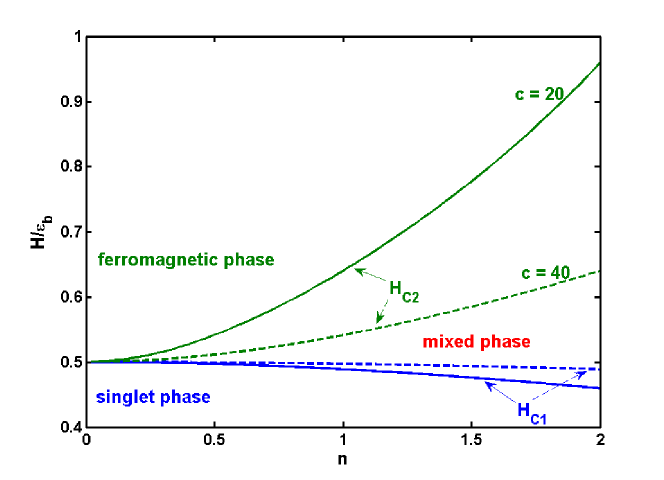
Figure 3: Phase diagram in plane $(n,H)$ for different values of interaction strength $c$.

In Fig. 3, we show the ground-state phase diagram in the $n-H$ plane. As $n\to 0$, both critical fields approach the same value $H_{c}=\epsilon_{\rm b}/2$. The solid (dashed) lines correspond to the two critical fields for the case $c=20$ ($c=40$). The ferromagnetic phase of all atoms in state $\left|F=1,m_{F}=1\right\rangle$ appears above the critical field $H_{c2}$, the singlet phase of singlet pairs appears below the critical field $H_{c1}$ and the mixed phase of atoms in state $\left|F=1,m_{F}=1\right\rangle$ and singlet pairs appears between the two critical fields.

V The spin and charge velocities

In 1D systems, spin-charge separation is the hallmark of many-body physics Giamarchi2003 . The collective charge excitations are described by sound modes with a linear dispersion. The spin excitations are gapped with a dispersion $\epsilon_{\nu}(p)=\sqrt{\Delta_{\nu}^{2}+v_{\nu}^{2}p^{2}}$ where $\Delta_{\nu}$ is the excitation gap and $v_{\nu}$ is the spin velocity in spin branch $\nu$. This leads to the phenomenon of spin-charge separation. A method has been proposed to probe this phenomenon experimentally in a 1D system of interacting electrons at low energies Jompol2009 .

To calculate the charge velocity, we need to find the energy of the lowest excited state that does not involve breaking any pairs. In the absolute ground state where $H=0$, the system is only made up of fully paired states below the “Fermi level” and the total momentum of the system is zero. This is achieved when there is no magnetic field present. To excite the system, we allow the pair with the largest momentum to leave the “Fermi sea” and let the excited state have a total momentum of $p$, i.e., $\sum_{j}k_{j}=p$. We then calculate its total energy $E=\sum_{j}k_{j}^{2}$. The difference between the excitation energy and the ground state energy is equal to the charge velocity times $p$. The energy difference in the thermodynamic limit is thus calculated to be

$$E(p)-E_{0}=\pi n_{2}p\left(1+\frac{2n_{2}}{3c}\right)+O\left(\frac{1}{c^{2}}\right).$$ (19)

Therefore in terms of the total particle number $n=N/L$ and interaction strength $c$, the charge velocity is

$$v_{c}=\frac{\pi n}{2}\left(1+\frac{1}{3\gamma}\right)+O\left(\frac{1}{c^{2}}\right).$$ (20)

An alternative way to calculate the charge velocity for the singlet ground state is through the relation

$$v_{c}=\sqrt{\frac{2L}{n}\left(\frac{\partial^{2}E_{0}}{\partial L^{2}}\right)}.$$ (21)

Both methods yield the same result.

The spin velocity on the other hand is calculated by considering the lowest excited state where one pair is broken into two unpaired states. Both unpaired states will occupy opposite ends of the momentum distribution so that the excitation energy is minimized. The total momentum of the excited state can be parameterized by $p$ in the same manner as before. We can equate the energy difference between the excited state and the fully paired ground state to the energy dispersion $\epsilon(p)$. In the thermodynamic limit,

$$E(p)-E_{0}=\frac{c^{2}}{8}+\frac{p^{2}}{2}\left(1+\frac{64n_{2}}{5c}\right)+O\left(\frac{1}{c^{2}}\right)\equiv\epsilon(p).$$ (22)

From the original relation $\epsilon(p)=\sqrt{\Delta^{2}+v_{s}^{2}p^{2}}$, we obtain the relation $\epsilon(p)=\Delta+\frac{v_{s}^{2}p^{2}}{2\Delta}$ in the limit $\Delta\gg 1$ where the gap is very large. Comparing both expressions for the dispersion energy, we can easily verify that $\Delta=c^{2}/8$ and

$$v_{s}^{2}=\frac{c^{2}}{8}\left(1+\frac{64n_{2}}{5c}\right).$$ (23)

Hence the spin velocity is

$$v_{s}=\frac{c}{2\sqrt{2}}\left(1+\frac{16n}{5c}\right)+O\left(\frac{1}{c^{2}}\right).$$ (24)

The spin velocity is divergent due to a large energy gap as $c\to\infty$. This demonstrates that there is spin-charge separation over the singlet ground state. We also note that this phenomenon depends on the state of the system within an external field. Essler et al. Essler2009 showed that spin and charge velocities are equal in the weak coupling limit when there is no external field involved.

In the gapless phase when $H_{c1}<H<H_{c2}$, the ground state ($T\rightarrow 0$) of this system is conformally invariant Blote1986 ; Affleck1986 . The excitations close to the “Fermi surfaces” in unpaired and pair branches have linear dispersions. The finite-size corrections to the ground state energy are given by

$$E_{0}=Le_{0}^{\infty}-\frac{\pi c}{6L}(v_{c}^{(1)}+v_{c}^{(2)})$$ (25)

where the central charge $c=1$ for this system, $E_{0}$ is the ground state energy for the finite system and $e_{0}^{\infty}$ is the ground state energy density for the infinite system. The charge velocities for unpaired and paired bosons are given explicitly by the expressions

$$v_{c}^{(1)} \approx 2\pi n_{1}\left(1+\frac{2(32n_{2}-10n_{1})}{5c}+\frac{3(32n_{2}-10n_{1})^{2}}{25c^{2}}\right),$$

$$v_{c}^{(2)} \approx \pi n_{2}\left(1+\frac{2(48n_{1}+5n_{2})}{15c}+\frac{3(48n_{1}+5n_{2})^{2}}{225c^{2}}\right).$$ (26)

In this phase, spin fluctuations are frozen out and thus the charge density fluctuations dominate the ground state and is effectively described by the universality class of a two component Luttinger liquid.

VI Conclusion

In conclusion we derived the TBA equations for a system of 1D spin-1 bosons with repulsive density-density and antiferromagnetic spin exchange interactions and solved the TBA equations for the zero temperature case in the strong coupling limit. We obtained the ground state energy, chemical potentials, critical fields and magnetization in terms of interaction strength and the external magnetic field. We also presented an exact phase diagram of strongly interacting spin-1 bosons which facilitates experimental analysis of phase segments. For the weak coupling limit, the collective excitations in the charge sector is described by a Tomonaga-Luttinger liquid, whereas the spin dynamics is described by the $O(3)$ non-linear sigma model Essler2009 . However, for the strong coupling limit, spin fluctuations can be suppressed by a strong external magnetic field. The density fluctuations thus evolve into a two-component Luttinger liquid. At zero temperature, the model exhibits three quantum phases: singlet pairs of two bosons for external field $H<H_{c1}$; a fully-polarized Tonks-Girardeau gas phase of $m_{F}=1$ bosons for $H>H_{c2}$; and a mixed phase of singlet pairs and unpaired $m_{F}=1$ atoms for an intermediate field $H_{c1}<H<H_{c2}$. The phase transitions in the vicinities of $H_{c1}$ and $H_{c2}$ are of second order with a linear-field-dependent magnetization. Our results provide a new aspect of this model, namely spin liquid v.s. Luttinger liquid behavior.

This work has been supported by the Australian Research Council. We thank Profs J.-P. Cao, S. Chen and Y.-P. Wang for helpful discussions. C.L. thanks Yu.S. Kivshar for support.

Appendix A Derivation of the TBA Equations

Here we derive the TBA equations in detail following the steps for the attractive spin-1/2 fermion model in Chapter 13 of Takahashi’s book Takahashi1999 . Substituting all possible solutions for $\{k_{j}\}$ and $\{\Lambda_{\alpha}\}$ back into the BA equations (2) gives

$$\exp(\mathrm{i}k_{j}L) = \prod_{l\neq j}^{N_{1}}e_{4}(k_{j}-k_{l})\prod_{l=1}^{N_{2}}e_{-1}(k_{j}-\lambda_{l})e_{5}(k_{j}-\lambda_{l})$$ (27)

$$\prod_{n=1}^{\infty}\prod_{\alpha=1}^{M_{n}}e_{-(n-1)}(k_{j}-\Lambda_{\alpha}^{n})$$

$$\prod_{n=1}^{\infty}\prod_{\alpha=1}^{M_{n}}e_{-(n+1)}(k_{j}-\Lambda_{\alpha}^{n}),$$

$$\exp(\mathrm{i}2\lambda_{j}L) = \prod_{l=1}^{N_{1}}e_{-1}(\lambda_{j}-k_{l})e_{5}(\lambda_{j}-k_{l})$$ (28)

$$\prod_{l\neq j}^{N_{2}}e_{-2}(\lambda_{j}-\lambda_{l})e_{4}(\lambda_{j}-\lambda_{l})e_{6}(\lambda_{j}-\lambda_{l}),$$

$$\prod_{l=1}^{N_{1}}e_{(n-1)}(\Lambda_{\alpha}^{n}-k_{l})e_{(n+1)}(\Lambda_{\alpha}^{n}-k_{l})$$ (29)

$$=-\prod_{m=1}^{\infty}\prod_{\beta=1}^{M_{m}}E_{mn}(\Lambda_{\alpha}^{n}-\Lambda_{\beta}^{m}),$$

where $E_{mn}(x)$ is defined as

$$E_{mn}(x)=\left\{\begin{array}[]{lll}e_{|m-n|}(x)e_{|m-n|+2}^{2}(x)\ldots\\ e_{m+n-2}^{2}(x)e_{m+n}(x),&\hbox{for $n\neq m$,}\\ e_{2}^{2}(x)e_{4}^{2}(x)\ldots\\ e_{2n-2}^{2}(x)e_{2n}(x),&\hbox{for $n=m$.}\\ \end{array}\right.$$ (30)

Following the technique pioneered by Yang and Yang Yang1969 for spinless bosons, the logarithm of equations (A1) to (A3) then gives

$$k_{j}L = 2\pi I_{j}-\sum_{l\neq j}^{N_{1}}\theta\left(\frac{k_{j}-k_{l}}{4c^{\prime}}\right)$$ (31)

$$+\sum_{l=1}^{N_{2}}\left[\theta\left(\frac{k_{j}-\lambda_{l}}{c^{\prime}}\right)-\theta\left(\frac{k_{j}-\lambda_{l}}{5c^{\prime}}\right)\right]$$

$$+\sum_{n=1}^{\infty}\sum_{\alpha=1}^{M_{n}}\left[\theta\left(\frac{k_{j}-\Lambda_{\alpha}^{n}}{(n-1)c^{\prime}}\right)+\theta\left(\frac{k_{j}-\Lambda_{\alpha}^{n}}{(n+1)c^{\prime}}\right)\right],$$

$$2\lambda_{j}L = 2\pi J_{j}+\sum_{l=1}^{N_{1}}\left[\theta\left(\frac{\lambda_{j}-k_{l}}{c^{\prime}}\right)-\theta\left(\frac{\lambda_{j}-k_{l}}{5c^{\prime}}\right)\right]$$ (32)

$$+\sum_{l\neq j}^{N_{2}}\left[\theta\left(\frac{\lambda_{j}-\lambda_{l}}{2c^{\prime}}\right)-\theta\left(\frac{\lambda_{j}-\lambda_{l}}{4c^{\prime}}\right)\right.$$

$$\left.-\theta\left(\frac{\lambda_{j}-\lambda_{l}}{6c^{\prime}}\right)\right],$$

$$\sum_{l=1}^{N_{1}}\left[\theta\left(\frac{\Lambda_{\alpha}^{n}-k_{l}}{(n-1)c^{\prime}}\right)+\theta\left(\frac{\Lambda_{\alpha}^{n}-k_{l}}{(n+1)c^{\prime}}\right)\right]$$ (33)

$$=2\pi L_{\alpha}^{n}+\sum_{m=1}^{\infty}\sum_{\beta=1}^{M_{m}}\Theta_{mn}\left(\frac{\lambda_{\alpha}^{n}-\Lambda_{\beta}^{m}}{c^{\prime}}\right),$$

where $\theta(x)=2\tan^{-1}(x)$ and

$$\Theta_{mn}(x)=\left\{\begin{array}[]{lll}\theta\left(\frac{x}{|m-n|}\right)+2\theta\left(\frac{x}{|m-n|+2}\right)+\ldots\\ +2\theta\left(\frac{x}{m+n-2}\right)+\theta\left(\frac{x}{m+n}\right),&\hbox{for $n\neq m$,}\\ 2\theta\left(\frac{x}{2}\right)+2\theta\left(\frac{x}{4}\right)+\ldots\\ +2\theta\left(\frac{x}{2n-2}\right)+\theta\left(\frac{x}{2n}\right),&\hbox{for $n=m$.}\\ \end{array}\right.$$ (34)

Writing the occupied distribution functions of the unpaired $k$’s, the paired $k$’s and the $\Lambda$-strings as $\rho_{1}(k)$, $\rho_{2}(k)$ and $\sigma_{n}(k)$ and their corresponding unoccupied distribution functions as $\rho_{1}^{h}(k)$, $\rho_{2}^{h}(k)$ and $\sigma_{n}^{h}(k)$, we take the thermodynamic limit of the above equations to obtain the integral equations

$$\rho_{1}(k)+\rho_{1}^{h}(k) = \frac{1}{2\pi}+a_{4}\ast\rho_{1}(k)$$ (35)

$$+[a_{5}-a_{1}]\ast\rho_{2}(k)$$

$$-\sum_{n=1}^{\infty}[a_{n-1}+a_{n+1}]\ast\sigma_{n}(k),$$

$$\rho_{2}(k)+\rho^{h}_{2}(k) = \frac{1}{\pi}+[a_{5}-a_{1}]\ast\rho_{1}(k)$$ (36)

$$+[a_{6}+a_{4}-a_{2}]\ast\rho_{2}(k),$$

$$\sigma_{n}(k)+\sigma_{n}(k) = [a_{n-1}+a_{n+1}]\ast\rho_{1}(k)$$ (37)

$$-\sum_{m=1}^{\infty}T_{mn}\ast\sigma_{m}(k),$$

where

$$f\ast g(x)=\int_{-\infty}^{\infty}f(x-x^{\prime})g(x^{\prime})dx^{\prime},$$ (38)

$$a_{n}(x)=\frac{1}{\pi}\frac{n|c^{\prime}|}{(nc^{\prime})^{2}+x^{2}},$$ (39)

and

$$T_{mn}(x)=\left\{\begin{array}[]{ll}a_{|m-n|}(x)+2a_{|m-n|+2}(x)+\ldots\\ +2a_{m+n-2}(x)+a_{m+n}(x),&\hbox{for $n\neq m$,}\\ 2a_{2}(x)+2a_{4}(x)+\ldots\\ +2a_{2n-2}(x)+a_{2n}(x),&\hbox{for $n=m$.}\\ \end{array}\right.$$ (40)

The distribution functions are related to the particle numbers via the relations

$$n_{1} = \frac{N_{1}}{L}=\int_{-\infty}^{\infty}\rho_{1}(k)dk,$$ (41)

$$n_{2} = \frac{N_{2}}{L}=\int_{-\infty}^{\infty}\rho_{2}(k)dk,$$ (42)

$$m = \sum_{n=1}^{\infty}n\int_{-\infty}^{\infty}\sigma_{n}(k)dk.$$ (43)

The total number of microstates in an interval $dk$ is

$$dW = \frac{(L(\rho_{1}(k)+\rho_{1}^{h}(k))dk)!}{(L\rho_{1}(k)dk)!(L\rho_{1}^{h}(k)dk)!}$$ (44)

$$\times\frac{(L(\rho_{2}(k)+\rho_{2}^{h}(k))dk)!}{(L\rho_{2}(k)dk)!(L\rho_{2}^{h}(k)dk)!}$$

$$\times\prod_{n=1}^{\infty}\frac{(L(\sigma_{n}(k)+\sigma_{n}^{h}(k))dk)!}{(L\sigma_{n}(k)dk)!(L\sigma_{n}^{h}(k)dk)!}.$$

Through the use of Stirling’s approximation, the entropy is written as

$$\frac{S}{L} = \int_{-\infty}^{\infty}\left[(\rho_{1}+\rho_{1}^{h})\ln(\rho_{1}+\rho_{1}^{h})\right.$$ (45)

$$\left.-\rho_{1}\ln\rho_{1}-\rho_{1}^{h}\ln\rho_{1}^{h}\right]dk$$

$$+\int_{-\infty}^{\infty}\left[(\rho_{2}+\rho_{2}^{h})\ln(\rho_{2}+\rho_{2}^{h})\right.$$

$$\left.-\rho_{2}\ln\rho_{2}-\rho_{2}^{h}\ln\rho_{2}^{h}\right]dk$$

$$+\sum_{n=1}^{\infty}\int_{-\infty}^{\infty}\left[(\sigma_{n}+\sigma_{n}^{h})\ln(\sigma_{n}+\sigma_{n}^{h})\right.$$

$$\left.-\sigma_{n}\ln\sigma_{n}-\sigma_{n}^{h}\ln\sigma_{n}^{h}\right]dk.$$

The Gibbs free energy per unit length is

$$\Omega=\frac{E}{L}-\mu n-\frac{TS}{L}+\frac{E_{z}}{L}$$ (46)

where $\mu$ is the chemical potential, the energy per unit length is

$$\frac{E}{L}=\int_{-\infty}^{\infty}k^{2}\rho_{1}(k)dk+\int_{-\infty}^{\infty}(2k^{2}-2c^{\prime 2})\rho_{2}(k)dk$$ (47)

and the Zeeman energy per unit length is given in terms of the external magnetic field $H$

$$\frac{E_{z}}{L}=-H\int_{-\infty}^{\infty}\rho_{1}(k)dk+H\sum_{n=1}^{\infty}n\int_{-\infty}^{\infty}\sigma_{n}(k)dk.$$ (48)

Minimizing the Gibbs free energy and going through a similar procedure as shown in Takahashi1999 , we arrive finally at the TBA equations (4).

Figure 1: (color online) Schematic configuration of the quasimomenta $k$ and spin rapidities $\Lambda$ in the complex plane for the ground state in the strong coupling limit with $N=17$ and $M=12$. Dashed boundaries indicate pair formations with the same real parts. Each pair in $k$-space has a corresponding pair in $\Lambda$-space. As mentioned in the text, the individual particle numbers for $m_{F}=0,\pm 1$ are not conserved and thus can fluctuate.

Figure 2: Normalized magnetization $m^{z}$ versus re-scaled magnetic field $H/\epsilon_{b}$ for different values of interaction strength $c$.

References

• (1) D. M. Stamper-Kurn, M. R. Andrews, A. P. Chikkatur, S. Inouye, H.-J. Miesner, J. Stenger and W. Ketterle, Phys. Rev. Lett. 80, 2027 (1998)
• (2) H.-J. Miesner, D. M. Stamper-Kurn, J. Stenger, S. Inouye, A. P. Chikkatur and W. Ketterle, Phys. Rev. Lett. 82, 2228 (1999)
• (3) M. R. Matthews, B. P. Anderson, P. C. Haljan, D. S. Hall, C. E. Wieman and E. A. Cornell, Phys. Rev. Lett. 83, 2498 (1999)
• (4) M. D. Barrett, J. A. Sauer and M. S. Chapman, Phys. Rev. Lett. 87, 010404 (2001)
• (5) T. Ohmi and K. Machida, J. Phys. Soc. Jpn. 67, 1822 (1998)
• (6) T. L. Ho, Phys. Rev. Lett. 81, 742 (1998)
• (7) J. Stenger, S. Inouye, D. M. Stamper-Kurn, H.-J. Miesner, A. P. Chikkatur and W. Ketterle, Nature 396, 345 (1998)
• (8) T. Isoshima, K. Machida and T. Ohmi, Phys. Rev. A 60, 4857 (1999)
• (9) C. K. Law, H. Pu and N. P. Bigelow, Phys. Rev. Lett. 81, 5257 (1998)
• (10) H. Pu, C. K. Law, S. Raghavan, J. H. Eberly, and N. P. Bigelow, Phys. Rev. A 60, 1463 (1999)
• (11) T. L. Ho and S. K. Yip, Phys. Rev. Lett. 84, 4031 (2000)
• (12) Matteo Rizzi, Davide Rossini, Gabriele De Chiara, Simone Montangero and Rosario Fazio, Phys. Rev. Lett. 95, 240404 (2005)
• (13) A. Imambekov, M. Lukin and E. Demler, Phys. Rev. A 68, 063602 (2003)
• (14) S. K. Yip, Phys. Rev. Lett. 90, 250402 (2003)
• (15) E. Demler and F. Zhou, Phys. Rev. Lett. 88, 163001 (2002)
• (16) E. Eisenberg and E. H. Lieb, Phys. Rev. Lett. 89, 220403 (2002)
• (17) K. Yang and Y.-Q. Li, Int. J. Mod. B 17, 1027 (2003)
• (18) X.-W. Guan, M. T. Batchelor and M. Takahashi, Phys. Rev. A 76, 043617 (2007)
• (19) M. Koashi and M. Ueda, Phys. Rev. Lett. 84, 1066 (2000)
• (20) J. Cao, Y. Jiang and Y. Wang, Europhys. Lett. 79, 30005 (2007)
• (21) F. H. L. Essler, G. V. Shlyapnikov and A. M. Tsvelik, J. Stat. Mech. P02027 (2009)
• (22) F. Zhou, Phys. Rev. Lett. 87, 080401 (2001)
• (23) C. N. Yang and C. P. Yang, J. Math. Phys. 10, 1115 (1969)
• (24) M. Takahashi, Prog. Theor. Phys. 46, 401 (1971)
• (25) M. Takahashi, Thermodynamics of One-Dimensional Solvable Models, Cambridge University Press (1999)
• (26) X.-W. Guan, M. T. Batchelor, C. Lee and M. Bortz, Phys. Rev. B 76, 085120 (2007)
• (27) T. Iida and M. Wadati, J. Stat. Mech. P06011 (2007)
• (28) E. Zhao, X.-W. Guan, W. Vincent Liu, M. T. Batchelor and M. Oshikawa, arXiv:0907.3198.
• (29) J.-S. He, A. Foerster, X.-W. Guan, M. T. Batchelor, New J. Phys. 11, 073009 (2009)
• (30) M. T. Batchelor, X.-W. Guan, N. Oelkers and Z. Tsuboi, Adv. Phys. 56, 465 (2007)
• (31) T. Giamarchi, Quantum Physics in One Dimension, Oxford University Press (2003)
• (32) Y. Jompol, C. J. B. Ford, J. P. Griffiths, I. Farrer, G. A. C. Jones, D. Anderson, D. A. Ritchie, T. W. Silk and A. J. Schofield, Science 325, 597 (2009)
• (33) H. W. J. BlΓΆte, J. L. Cardy and M. P. Nightingale, Phys. Rev. Lett. 56, 742 (1986)
• (34) I. Affleck, Phys. Rev. Lett. 56, 746 (1986)
Refer to caption