Renormalization group study of Luttinger liquids with boundaries

Abstract

We use Wilsons weak coupling “momentum” shell renormalization group method to show that two-particle interaction terms commonly neglected in bosonization of one-dimensional correlated electron systems with open boundaries are indeed irrelevant in the renormalization group sense. Our study provides a more solid ground for many investigations of Luttinger liquids with open boundaries.

Introduction—The electron-electron interaction has strong effects on the low-energy physics of (quasi) one-dimensional (1d) metals. Such systems cannot be described within Landaus Fermi liquid (FL) theory but rather form a different “universality” class: the Luttinger liquids (LLs).Schoenhammer05 Already decades ago the importance of local single-particle inhomogeneities in LLs allowing for electron backscattering with momentum transfer $2k_{F}$ (were $k_{F}$ is the Fermi momentum) was emphasized.LutherPeschel ; Mattis Their relevance became even more apparent after it was shown that on low energy scales a LL (with repulsive two-particle interaction) with a single local impurity in many respects behaves as if the chain was cut in two at the position of the impurity with open boundary conditions at the endpoints.KaneFisher ; Furusaki0 This led to a number of studies on the physics of LLs with open boundariesFG ; EMJ ; WVP ; VWG ; MMX mainly using the method of bosonization.Schoenhammer05 ; Herbert

The Tomonaga-Luttinger modelSchoenhammer05 is a translationally invariant (no inhomogeneities) continuum model within the LL “universality” class for which all correlation functions can be computed exactly by bosonization. In the context of bulk LL physics it plays a role similar to the noninteracting electron gas for FL physics.Schoenhammer05 In this model the $2k_{F}$ two-particle scattering process of spin-up and spin-down electrons is neglected. All the other low-energy scattering process can be written as quadratic forms in the bosonic densities of the right- (around $k_{F}$) and left-moving (around $-k_{F}$) fermions. Furthermore, after linearization of the single-particle dispersion, also the kinetic energy is quadratic in the bosonic densitiesSchoenhammer05 ; Herbert and the remaining Hamiltonian is that of noninteracting bosons. Neglecting the above $2k_{F}$ scattering process leads to an additional conservation law, namely the “local” (in momentum space) spin around the two Fermi points $\pm k_{F}$, which is central to the exact solution of the Tomonaga-Luttinger model. In the literature one finds two arguments why this so-called $g_{1,\perp}$-term can be neglected. Either one follows the original idea of TomonagaTomonaga and assumes a two-particle interaction which is sufficiently smooth and long-ragend in real-space (suppressed screening) such that its Fourier component at $2k_{F}$ vanishes or, more generally, one adopts the so called g-ology renormalization group (RG) approach of Sólyom.solyom In this it is shown that in an important part of the parameter space $g_{1,\perp}$ is irrelevant in the RG sense. The solution $g_{1,\perp}=0$ is a stable fixed point of the RG flow.solyom To (qualitatively) understand the low-energy physics the $g_{1,\perp}$-term can thus be neglected. It only affects the numerical values of the other fixed-point couplings.foot1

For open boundary conditions the single-particle quantum number $k$ in which the noninteracting problem is diagonal (see below) no longer corresponds to the momentum. Therefore the two-particle scattering terms appearing in this natural basis have a form different from those of the translationally invariant case. Also for LLs with open boundary conditions the Hamiltonian contains two-particle scattering terms which cannot be written as quadratic forms in bosonic densities, when considering a general, spin-conserving two-particle interaction. It was shownMMX that these terms vanish if Tomonagas rather specific assumption of an interaction which is smooth in real-space is made. Then open-boundary bosonization can be used to compute all correlation functions of the open-boundary analog of the Tomonaga-Luttinger model.FG ; EMJ ; WVP ; VWG ; MMX ; Dirk Surprisingly, an RG analysis for more general two-particle interactions similar to Sólyoms approach was so far not discussed in the standard literature on open-boundary bosonization. In the present Brief Report we close this gap. Using Wilsons “momentum” shell RG in weak couplingfoot2 ; Shankar we show that all two-particle scattering terms naturally arising in a low-energy analysis of a 1d system with general two-particle interaction and open boundaries which cannot be written as quadratic forms in the bosonic densities are RG irrelevant (open boundary g-ology analysis). We demonstrate that the RG flow equations are the same as the ones of the translationally invariant g-ology model. In analogy to this the RG irrelevant coupling constants only affect the fixed-point couplings of the terms quadratic in the bosons and can thus be neglected for a qualitative understanding of the low-energy physics of LLs with open boundaries. Our analysis puts many of the studies of LLs with open boundaries on a more solid ground.

Model—To be specific we consider the 1d electron gas on a line between $x=0$ and $x=L$ with a general, sufficiently regular two-particle interaction

$$\hat{V} = \frac{1}{2}\sum_{s,s^{\prime}}\int^{L}_{0}\!\!\!\!dx\int^{L}_{0}\!\!\!\!dx^{\prime}\psi_{s}^{{\dagger}}(x)\psi_{s^{\prime}}^{{\dagger}}(x^{\prime})$$

$$\times V_{s,s^{\prime}}(x-x^{\prime})\psi_{s^{\prime}}(x^{\prime})\psi_{s}(x)$$

where $s,s^{\prime}$ denote the spin. The noninteracting one-particle eigenstates are given by standing waves (open boundaries) $\varphi_{n}(x)=\sqrt{2/L}\sin{(k_{n}x)}$, with quantum numbers $k_{n}=n\pi/L$, $n\in{\mathbb{N}}$. We emphasize that for open boundaries only right-moving electrons with a positive Fermi velocity $v_{F}=k_{F}/m_{e}$ appear, where $m_{e}$ denotes the electron mass. The field operator is given by $\psi_{s}^{({\dagger})}(x)=\sum_{n=1}^{\infty}\varphi_{n}(x)a^{(\dagger)}_{n,s}$ with the creation and annihilation operators $a^{({\dagger})}_{n,s}$ of electrons in the noninteracting eigenstates. We now closely follow Ref. MMX, to rewrite the interacting part of the Hamiltonian as

$$\hat{V}=\frac{1}{2}\sum_{s,s^{\prime}}\sum_{n,m,n^{\prime},m^{\prime}}v^{s,s^{\prime}}_{n,m,n^{\prime},m^{\prime}}a^{{\dagger}}_{n,s}a^{{\dagger}}_{m,s^{\prime}}a_{m^{\prime},s^{\prime}}a_{n^{\prime},s}$$

with the matrix elements

$$v_{n,m,n^{\prime},m^{\prime}}^{s,s^{\prime}}=\left[F_{s,s^{\prime}}\left(k_{n}-k_{n^{\prime}},k_{m}-k_{m^{\prime}}\right)\right.$$

$$-F_{s,s^{\prime}}\left(k_{n}-k_{n^{\prime}},k_{m}+k_{m^{\prime}}\right)-F_{s,s^{\prime}}\left(k_{n}+k_{n^{\prime}},k_{m}-k_{m^{\prime}}\right)$$

$$\left.+F_{s,s^{\prime}}\left(k_{n}+k_{n^{\prime}},k_{m}+k_{m^{\prime}}\right)\right]/L\;,$$ (1)

where

$$F_{s,s^{\prime}}(q,q^{\prime})=\frac{1}{L}\int^{L}_{0}\!\!\!\!dx\int^{L}_{0}\!\!\!\!dx^{\prime}\cos{(qx)}V_{s,s^{\prime}}(x-x^{\prime})\cos{(q^{\prime}x^{\prime})}\;.$$

The kinetic part of the Hamiltonian $\hat{H}=\hat{T}+\hat{V}$ is given by

$$\hat{T}=\sum_{s}\sum_{n}\epsilon_{k_{n}}a^{{\dagger}}_{n,s}a_{n,s}$$

with the single-particle dispersion $\epsilon_{k}=k^{2}/(2m_{e})$.

Perturbative Wilson RG—To analyze the Hamiltonian $\hat{H}$ using a Wilson RG we consider the action $S(\bar{\Psi},\Psi)$ appearing in the imaginary time functional integral representation of the grand canonical partition function

$$S(\bar{\Psi},\Psi)=S_{0}+S_{I}$$

$$=-\sum_{s}\sum_{n}\sum_{j}\bar{\Psi}_{s}(k_{n},\omega_{j})[{\mathcal{G}}_{0}(k_{n},\omega_{j})]^{-1}\Psi_{s}(k_{n},\omega_{j})$$

$$+\beta^{-1}\sum_{s,s^{\prime}}\sum_{n,m,n^{\prime},m^{\prime}}\sum_{i,j,i^{\prime},j^{\prime}}\delta_{i+j,i^{\prime}+j^{\prime}}v^{s,s^{\prime}}_{n,m,n^{\prime},m^{\prime}}$$

$$\times\bar{\Psi}_{s}(k_{n},\omega_{i})\bar{\Psi}_{s^{\prime}}(k_{m},\omega_{j})\Psi_{s^{\prime}}(k_{m^{\prime}},\omega_{j^{\prime}})\Psi_{s}(k_{n^{\prime}},\omega_{i^{\prime}})\;,$$

with Graßmann variables $\Psi$, $\bar{\Psi}$, Matsubara frequencies $\omega_{j}$, the noninteracting propagator ${\mathcal{G}}_{0}(k,\omega)=[i\omega-\epsilon_{k}+\mu]^{-1}$ ($\mu$ is the chemical potential), and the inverse temperature $\beta$. Here we will only be interested in the behavior at zero temperature ($\beta\to\infty$) with $\mu=\epsilon_{F}=k_{F}^{2}/(2m_{e})$. In this case we obtain $\epsilon_{k}-\mu=v_{F}(k-k_{F})+(k-k_{F})^{2}/(2m_{e})$.

We now follow the standard steps of the perturbative Wilson $k$-shell RG:Shankar (i) separating the Graßmann fields $\Psi=\Psi^{<}+\Psi^{>}$ into fast modes $\Psi^{>}$ (relative to the Fermi point) with $\Lambda/b\leq|k-k_{F}|\leq\Lambda$ and slow ones $\Psi^{<}$, (ii) integrating out the fast modes $\Psi^{>}$ perturbatively, (iii) rescaling the quantum numbers $\tilde{k}=k-k_{F}$ ($\tilde{k}^{\prime}=b\tilde{k}$) and the Matsubara frequencies ($\omega^{\prime}=b\omega$)foot3 and (iv) rescaling the Graßmann fields $\Psi^{\prime}(\tilde{k}^{\prime}+k_{F},\omega^{\prime})=\xi^{-1}\Psi^{<}(\tilde{k}^{\prime}/b+k_{F},\omega^{\prime}/b)$.

We first consider the noninteracting case. Then the action can naturally be written as $S_{0}=S_{0}^{<}(\bar{\Psi}^{<},\Psi^{<})+S_{0}^{>}(\bar{\Psi}^{>},\Psi^{>})$ and the second step of the RG procedure only leads to a constant in the partition function. Therefore the rescaling is the only relevant step. Choosing $\xi=b^{1/2}$ the $i\omega-v_{F}(k-k_{F})$ part of the noninteracting action remains invariant, while the quadratic term of the dispersion vanishes as $1/b$ for large $b$. It is RG irrelevant for the low-energy physics and from now on we work with ${\mathcal{G}}_{0}(k,\omega)=[i\omega-v_{F}(k-k_{F})]^{-1}$. The standard linearization can thus be justified by the RG. Note that to avoid proliferation of symbols we do not introduce a new one for the free propagator of the model with linearized dispersion.

Next we study the flow of the quartic part of the action. As usual in a weak coupling RG to compute $\left<e^{-S_{I}}\right>_{S_{0}^{>}}$, where the index refers to taking the expectation value with respect to the fast mode part of the noninteracting action, we use a cumulant expansion

$$\ln\left<e^{-S_{I}}\right>_{S_{0}^{>}}=-\left<S_{I}\right>_{S_{0}^{>}}+\frac{1}{2}\left(\left<S_{I}^{2}\right>_{S_{0}^{>}}-\left<S_{I}\right>_{S_{0}^{>}}^{2}\right)+\ldots\;.$$

On tree level (first term of the above expansion) and for low energy scales ($b\to\infty$) the RG steps lead similarly to the translational invariant case to a two-particle interaction which is purely local in real space $V_{s,s^{\prime}}(x-x^{\prime})\to V_{s,s^{\prime}}(0)\delta(x-x^{\prime})$. All correction terms are subleading.Shankar Then the integrals in Eq. (LABEL:Fdef) can be performed leading to

$$F_{s,s^{\prime}}(q,q^{\prime})=V_{s,s^{\prime}}(0)\left(\delta_{q,q^{\prime}}+\delta_{q,-q^{\prime}}\right)/2\;.$$

This has to be contrasted to the case with periodic boundary conditions in which only the second Kronecker delta appears and the interaction matrix element only has the contribution coming from $F_{s,s^{\prime}}(k_{n}-k_{n^{\prime}},k_{m}-k_{m^{\prime}})$ with $k$ being the momentum.MMX Since for open boundaries all the incoming and outgoing quantum numbers must be close to the single Fermi point only the Kronecker deltas $\delta_{n-{n^{\prime}},m-{m^{\prime}}},\delta_{n-{n^{\prime}},-m+{m^{\prime}}}$, and $\delta_{n+{n^{\prime}},m+{m^{\prime}}}$ in the expression Eq. (1) for the interaction matrix element contribute. As in the translationally invariant g-ology model we now generalize the interaction and assume different coupling constants for each of the remaining low-energy scattering processes and each of the relative spin orientations of the two particles. Doing so one can expect that the following low-energy RG analysis is applicable not only to the electron gas model but also of relevance for a larger class of models, including lattice ones. For the interaction matrix element Eq. (1) this leads to

$$2Lv_{n,m,n^{\prime},m^{\prime}}^{s,s^{\prime}} = (\sideset{{}_{||}}{{}_{1}}{\mathop{g}}\delta_{s,s^{\prime}}+\sideset{{}_{\perp}}{{}_{1}}{\mathop{g}}\delta_{s,-s^{\prime}})\delta_{n+{n^{\prime}},m+{m^{\prime}}}$$

$$+(\sideset{{}_{||}}{{}_{2}}{\mathop{g}}\delta_{s,s^{\prime}}+\sideset{{}_{\perp}}{{}_{2}}{\mathop{g}}\delta_{s,-s^{\prime}})\delta_{n-{n^{\prime}},m-{m^{\prime}}}$$

$$+\left(\sideset{{}_{||}}{{}_{4}}{\mathop{g}}\delta_{s,s^{\prime}}+\sideset{{}_{\perp}}{{}_{4}}{\mathop{g}}\delta_{s,-s^{\prime}}\right)\delta_{n-{n^{\prime}},-m+{m^{\prime}}}\;.$$

The initial values of the generalized coupling constants are functions of the microscopic parameters of the underlying model. The relation between these two parameter sets can (in principle) be determined by an additional RG step or simpler by perturbation theory. For the coupling constants we use the same notationsolyom $g_{1}$, $g_{2}$ and $g_{4}$ as in the translationally invariant g-ology model,foot4 while we still make clear that we are dealing with a different situation by putting the spin orientation index to the left of the $g$’s.relspin Two reasons for this become clear already at this stage of the discussion. In analogy to the standard g-ology the $\sideset{{}_{\perp}}{{}_{1}}{\mathop{g}}$-term is the one which cannot be written as a quadratic form in the bosonic density operators of the right-moving electrons (for a detailed discussion on this, see Ref. MMX, ). Also in strict analogy the $\sideset{{}_{||}}{{}_{2}}{\mathop{g}}$- and $\sideset{{}_{||}}{{}_{1}}{\mathop{g}}$-terms describe the same scattering processes (as can be seen by reordering Graßmann fields and renaming indices in the expression for $S$) and could be combined in a single coupling constant $\sideset{{}_{||}}{{}_{2}}{\mathop{g}}-\sideset{{}_{||}}{{}_{1}}{\mathop{g}}$ (see also the RG flow equations below).

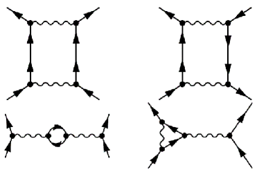
Figure 1: Topology of the second order diagrams contributing to the RG flow.

With these interaction matrix elements one now has to compute all (second order) connected diagrams of the two-particle vertex related to the second term of Eq. (LABEL:cumu) with all the external quantum numbers $k$ set to $k_{F}$ and the Matsubara frequencies set to zero. Writing down the corresponding analytical expressions it becomes immediately clear that only the one-particle irreducible diagrams give nonvanishing contributions. Furthermore, in complete analogy to the g-ology RG of the translationally invariant model to leading order the $g_{4}$-terms do not contribute to the RG flow of the coupling constants (they do not lead to $\ln(b)$-terms) and do not flow themself. They only lead to a renormalization of the Fermi velocity, which is a higher order effect if the RG flow of the couplings is considered. We thus neglect the $g_{4}$-term. In a straight forward but tedious calculation we evaluated all the remaining second order diagrams with the topologies as shown in Fig. 1. The wiggled line stands for any of the four coupling constants $\sideset{{}_{||}}{{}_{1}}{\mathop{{\gamma}}}$, $\sideset{{}_{\perp}}{{}_{1}}{\mathop{{\gamma}}}$, $\sideset{{}_{||}}{{}_{2}}{\mathop{{\gamma}}}$, and $\sideset{{}_{\perp}}{{}_{2}}{\mathop{{\gamma}}}$. We identified if a certain diagram gives a finite RG flow of the vertex and if so to which of the four scattering channels it contributes. To perform the remaining $k$-sum we took the limit $L\to\infty$ (resulting in a semi-infinite chain). Setting $b=e^{s}$ and resorting to infinitesimal RG steps this leads to the RG flow equations

$$\frac{d}{ds}\sideset{{}_{||}}{{}_{1}}{\mathop{{\gamma}}} = -\left({\sideset{{}_{||}}{{}_{1}}{\mathop{{\gamma}}}}^{2}+{\sideset{{}_{\perp}}{{}_{1}}{\mathop{{\gamma}}}}^{2}\right)\;,$$

$$\frac{d}{ds}\sideset{{}_{||}}{{}_{2}}{\mathop{{\gamma}}} = -{\sideset{{}_{||}}{{}_{1}}{\mathop{{\gamma}}}}^{2}\;,$$

$$\frac{d}{ds}\sideset{{}_{\perp}}{{}_{1}}{\mathop{{\gamma}}} = -2\sideset{{}_{\perp}}{{}_{1}}{\mathop{{\gamma}}}\left(\sideset{{}_{\perp}}{{}_{2}}{\mathop{{\gamma}}}-\sideset{{}_{||}}{{}_{2}}{\mathop{{\gamma}}}+\sideset{{}_{||}}{{}_{1}}{\mathop{{\gamma}}}\right)\;,$$

$$\frac{d}{ds}\sideset{{}_{\perp}}{{}_{2}}{\mathop{{\gamma}}} = -{\sideset{{}_{||}}{{}_{1}}{\mathop{{\gamma}}}}^{2}\;,$$ (4)

with

$$\sideset{{}_{\nu}}{{}_{l}}{\mathop{{\gamma}}}=\frac{\sideset{{}_{\nu}}{{}_{l}}{\mathop{{g}}}}{\pi v_{F}}$$

for $\nu=||,\perp$ and $l=1,2$. The coupling constants $\gamma$ are now understood to be functions of the infrared cutoff parameter $s$.

Remarkably, these equations are exactly the lowest-order RG flow equations for the coupling constants (divided by $2\pi v_{F}$ instead of $\pi v_{F}$) of the translationally invariant g-ology model.solyom This provides the complete justification for the decision to use the same notation. For the solution of the RG equations and an analysis of the fixed points we can proceed as it is well documented in the literature.solyom We first introduce the coupling constant

$$\gamma_{1,2}=\sideset{{}_{||}}{{}_{1}}{\mathop{{\gamma}}}-\sideset{{}_{||}}{{}_{2}}{\mathop{{\gamma}}}+\sideset{{}_{\perp}}{{}_{2}}{\mathop{{\gamma}}}\;,$$

which leads to the RG flow equations

$$\frac{d}{ds}\gamma_{1,2} = -2{\sideset{{}_{\perp}}{{}_{1}}{\mathop{{\gamma}}}}^{2}\;,$$

$$\frac{d}{ds}\sideset{{}_{\perp}}{{}_{1}}{\mathop{{\gamma}}} = -2\sideset{{}_{\perp}}{{}_{1}}{\mathop{{\gamma}}}\gamma_{1,2}\;.$$

From this it becomes apparent that $\gamma_{1,2}^{2}-{\sideset{{}_{\perp}}{{}_{1}}{\mathop{{\gamma}}}}^{2}$ is invariant under the RG flow which implies that the RG trajectories form hyperbolas in the $\sideset{{}_{\perp}}{{}_{1}}{\mathop{{\gamma}}}$-$\gamma_{1,2}$-plane. The equations can easily be solved and trajectories are sketched in Fig. 2. If initially (for the initial cutoff) all coupling constants are small and $\gamma_{1,2}^{i}\geq\left|{\sideset{{}_{\perp}}{{}_{1}}{\mathop{{\gamma}}}}^{i}\right|$ holds they all stay small (the use of perturbative RG is justified) and the flow is towards a line of stable fixed points with

$${\sideset{{}_{\perp}}{{}_{1}}{\mathop{{\gamma}}}}^{\ast}=0\;,\;\;\;\gamma_{1,2}^{\ast}=\left([\gamma_{1,2}^{i}]^{2}-{[{\sideset{{}_{\perp}}{{}_{1}}{\mathop{{\gamma}}}}^{i}]}^{2}\right)^{1/2}\;,$$

$${\sideset{{}_{\perp}}{{}_{2}}{\mathop{{\gamma}}}}^{\ast}={\sideset{{}_{\perp}}{{}_{2}}{\mathop{{\gamma}}}}^{i}+\frac{1}{2}\left(\gamma_{1,2}^{\ast}-\gamma_{1,2}^{i}\right)$$ (5)

indicated by the dashed line in Fig. 2. Under the above restriction on the initial coupling constants the term which cannot be written as a quadratic form in the bosonic density is RG irrelevant. The initial value ${\sideset{{}_{\perp}}{{}_{1}}{\mathop{{\gamma}}}}^{i}$ of the $\sideset{{}_{\perp}}{{}_{1}}{\mathop{{\gamma}}}$-term only affects the fixed-point values of the other couplings.solyom The use of the open boundary analog of the Tomonaga-Luttinger model is then justified for studies on the low-energy physics and standard open-boundary bosonizationFG ; EMJ ; WVP ; VWG ; MMX can be used. This allows to compute all correlation functions.FG ; EMJ ; WVP ; VWG ; MMX In the resulting expressions the coupling constants $\sideset{{}_{\perp}}{{}_{2}}{\mathop{{\gamma}}}$, $\sideset{{}_{||}}{{}_{2}}{\mathop{{\gamma}}}$ and $\sideset{{}_{||}}{{}_{1}}{\mathop{{\gamma}}}$ must be replaced by the fixed-point values Eq. (5).

Figure 2: Sketch of the trajectories of the weak coupling RG flow in the $\sideset{{}_{\perp}}{{}_{1}}{\mathop{{\gamma}}}$-$\gamma_{1,2}$-plane ($X=\sideset{{}_{\perp}}{{}_{1}}{\mathop{{\gamma}}}$, $Y=\gamma_{1,2}$). The dashed line indicates a line of stable fixed points. The fixed points on the dashed-dotted line are unstable.

For a model in which the coupling constants on the initial scale of the weak coupling RG do not depend on the relative orientation of the spins of the two scattering electrons (like the electron gas model) one finds $\gamma_{1,2}=\sideset{{}_{||}}{{}_{1}}{\mathop{{\gamma}}}$ and $\sideset{{}_{\perp}}{{}_{1}}{\mathop{{\gamma}}}=\sideset{{}_{||}}{{}_{1}}{\mathop{{\gamma}}}$. Therefore the above condition on the initial couplings for reaching a stable fixed point reduces to the simple requirement that the interaction must be repulsive. In this case the trajectory in Fig. 2 flows to the origin.

Summary—We have shown that under quite general assumptions on the two-particle interaction the terms which are usually ignored in bosonization studies on LLs with open boundaries are indeed RG irrelevant. These terms which cannot be written as quadratic forms in the bosonic densities only affect the fixed-point values of the other couplings but do not modify the low-energy physics. For this analysis we have used a perturbative Wilson RG scheme. Although the scattering terms for open boundaries are of different nature than in the translationally invariant standard g-ology model we have shown that the RG equations have exactly the same form. Our result puts a large number of bosonization studies on LL with open boundaries on a more solid ground. The present discussion is limited to the weak coupling regime. Numerical studies show that a similar low-energy physics can also be found at larger (repulsive) couplings.MMX We finally note that exactly the same results can be obtained using the functional renormalization groupHM instead of the Wilson RG.dipl

Acknowledgments—We thank K. Schönhammer and S. Andergassen for very valuable discussions, C. Karrasch for careful reading of the manuscript, and the Deutsche Forschungsgemeinschaft for support (FOR723).

References

- (1) For a recent review on LL physics see K. Schönhammer in Strong Interactions in Low Dimensions, Eds.: D. Baeriswyl and L. Degiorgi, Kluwer Academic Publishers, Dordrecht (2005).
- (2) A. Luther and I. Peschel, Phys. Rev. B 9, 2911 (1974).
- (3) D.C. Mattis, J. Math. Phys. 15, 609 (1974).
- (4) C.L. Kane and M.P.A. Fisher, Phys. Rev. Lett. 68, 1220 (1992); Phys. Rev. B 46, 15233 (1992).
- (5) A. Furusaki and N. Nagaosa, Phys. Rev. B 47, 4631 (1993).
- (6) M. Fabrizio and A. Gogolin, Phys. Rev. B 51, 17827 (1995).
- (7) S. Eggert, H. Johannesson, and A. Mattsson, Phys. Rev. Lett. 76, 1505 (1996).
- (8) Y. Wang, J. Voit, and F.-C. Pu, Phys. Rev. B 54, 8491 (1996).
- (9) J. Voit, Y. Wang, and M. Grioni, Phys. Rev. B 61, 7930 (2000).
- (10) V. Meden, W. Metzner, U. Schollwöck, O. Schneider, T. Stauber, and K. Schönhammer, Eur. Phys. J. B 16, 631 (2000).
- (11) For the discussion of correlation functions in the presence of boundaries and a bulk energy gap see D. Schuricht, F.H.L. Essler, A. Jaefari, and E. Fradkin, Phys. Rev. Lett. 101, 086403 (2008).
- (12) For an introduction to bosonization see J. von Delft and H. Schoeller, Ann. Phys. (Leipzig) 7, 225 (1998).
- (13) S. Tomonaga, Prog. Theor. Phys. 5, 544 (1950).
- (14) J. Sólyom, Adv. Phys. 28, 201 (1979).
- (15) We here and in the following speak of “couplings” (and not of coupling functions) as the -dependence turns out to be RG irrelevant (besides the classification concerning the momentum transfer; or for the translational invariant case).solyom
- (16) For open boundaries the quantum number does not correspond to the momentum. In the following we thus speak of the “Wilson -shell RG”.
- (17) For a review on the application of Wilson RG to interacting Fermi systems see R. Shankar, Rev. Mod. Phys. 66, 129 (1994).
- (18) To obtain a fixed-point scenario rescaling of the Matsubara frequencies is mandatory.
- (19) The umklapp scattering term appearing in the translationally invariant g-ology model if an underlying half filled lattice model is assumedsolyom is irrelevant for our considerations.
- (20) We note that using the index for the couplings in which two electrons with antiparallel spin scatter is to some extend misleading. As this is the notation widely used in the literature we here nevertheless follow this convention.
- (21) M. Salmhofer and C. Honerkamp, Prog. Theor. Phys. 105, 1 (2001).
- (22) S. Grap, Diploma thesis, RWTH Aachen University (2009).