Testing Molecular-Cloud Fragmentation Theories: Self-Consistent Analysis of OH Zeeman Observations

Abstract

The ambipolar-diffusion theory of star formation predicts the formation of fragments in molecular clouds with mass-to-flux ratios greater than that of the parent-cloud envelope. By contrast, scenarios of turbulence-induced fragmentation do not yield such a robust prediction. Based on this property, Crutcher et al. (2009) proposed an observational test that could potentially discriminate between fragmentation theories. However, the analysis applied to the data severely restricts the discriminative power of the test: the authors conclude that they can only constrain what they refer to as the “idealized” ambipolar-diffusion theory that assumes initially straight-parallel magnetic field lines in the parent cloud. We present an original, self-consistent analysis of the same data taking into account the nonuniformity of the magnetic field in the cloud envelopes, which is suggested by the data themselves, and we discuss important geometrical effects that must be accounted for in using this test. We show quantitatively that the quality of current data does not allow for a strong conclusion about any fragmentation theory. Given the discriminative potential of the test, we urge for more and better-quality data.

1 Introduction

The ratio of the mass and magnetic flux of interstellar molecular clouds has received well-deserved observational attention in recent years (e.g., Crutcher 1999; Heiles & Crutcher 2005). For a cloud as a whole, the mass-to-flux ratio is an important input to the ambipolar-diffusion theory of fragmentation (or core formation) in molecular clouds (e.g., see Fiedler & Mouschovias 1992, eq. [8]; 1993, eq. [1c] and associated discussion). What the ambipolar-diffusion theory predicts is the mass-to-flux ratio of fragments (or cores) in molecular clouds and how this quantity evolves in time from typical densities $\simeq 10^{3}\,{\rm cm^{-3}}$ to densities $\simeq 10^{14}\,{\rm cm^{-3}}$ (Tassis & Mouschovias 2007). Observations have been in excellent quantitative agreement with the theoretical predictions in that the mass-to-flux ratio of cores is found to be supercritical by a factor 1 - 4 (Crutcher et al. 1994; Crutcher 1999 and correction by Shu et al. 1999, pp. 196 - 198; Ciolek & Basu 2000; Troland & Crutcher 2008; Falgarone et al. 2008). By contrast, simulations of turbulence-driven fragmentation do not find cores with systematically greater mass-to-flux ratios than those of their parent clouds (e.g., Lunttila et al. 2008). Therefore, the effort by Crutcher et al. (2009) (hereinafter CHT) to measure the variation of the mass-to-flux ratio from the envelopes to the cores of four molecular clouds and thereby constrain cloud-fragmentation theories is a much needed observational test.

The effort by CHT to measure the magnetic field in four cloud envelopes yielded mostly nondetections, allowing only the placement of weak upper limits. Also, the data are suggestive of spatial variations of the field in the cloud envelopes. This spatial variation must be explicitly treated in the data analysis. Instead, CHT performed an analysis based on the overly restrictive (and contradicted by the data) assumption of uniform magnetic field in the envelope, which minimizes the potentially constraining power of their observations. CHT attempt to justify their restrictive assumption by claiming that they are testing the “idealized ambipolar-diffusion model” that assumes initially straight-parallel field lines in the parent cloud. Thus, if the data and the data analysis in CHT are taken at face value, they at best test an input to a theory, not the prediction of the theory relating to the variation of the mass-to-flux ratio from a core to its envelope, given the field strength and its spatial variation in the envelope. As we show below, the geometry of the field lines in a parent cloud crucially affects the observed variation of the mass-to-flux ratio from a core to the envelope while the fundamental prediction of the ambipolar-diffusion theory (that the mass-to-flux ratio increases from the envelope to the core) remains unchanged.

In this letter, we present a novel analysis of the OH-Zeeman data, applicable also to other sets of data that show intrinsic variation of the quantity being measured.

2 Data Analysis

The CHT data consist of existing OH Zeeman measurements in four molecular cloud cores and of four new measurements in the region surrounding each of these cores (in the clouds L1448, B217-2, L1544, and B1). For each observation of an envelope’s line-of-sight magnetic field $B_{j}$, CHT quote an associated Gaussian uncertainty $\sigma_{j}$. These four values for each cloud envelope are shown in Table 1, col. 2 - 5 (taken from CHT Figs. 2 - 5).

Table 1: Magnetic Fields and Errors (in $\mu$G) in Four Cloud Envelopes (data from CHT).

Cloud	$B_{1}\pm\sigma_{1}$	$B_{2}\pm\sigma_{2}$	$B_{3}\pm\sigma_{3}$	$B_{4}\pm\sigma_{4}$
L1448CO	$-9\pm 13$	$-11\pm 6$	$-7\pm 7$	$14\pm 8$
B217-2	$-13\pm 9$	$5\pm 6$	$6\pm 8$	$9\pm 13$
L1544	$-3\pm 4$	$-1\pm 4$	$22\pm 6$	$2\pm 10$
B1	$-16\pm 6$	$0\pm 7$	$-3\pm 6$	$-10\pm 5$

2.1 The CHT Analysis

CHT assign a value to the magnetic field strength in each envelope, which is obtained from a simultaneous least-squares fit over the 8 Stokes V spectra (2 spectral lines at each of 4 positions in each envelope). The fit gives a single value of the line-of-sight field and a single value of its uncertainty in each envelope. The uncertainty was calculated under the assumption that there is no intrinsic spatial variation of the field strength in each cloud envelope and, therefore, any spread in the observed $B_{j}$ values is attributed to observational errors. The CHT values for the envelope fields and their uncertainties are shown in Table 2, column 2.

Using this mean field, CHT calculate what they regard as the magnetic flux of the envelope, which, combined with the flux in the core, is used to obtain the quantity $R$ defined by $R=\left(I_{\rm core}\Delta V_{\rm core}/{B_{\rm core}}\right)/\left(I_{\rm env}\Delta V_{\rm env}/{B_{\rm env}}\right)$. The quantity $I$ is the peak intensity of the spectral line in degrees K, $\Delta V$ is the FWHM in km $\rm s^{-1}$, and $B$ is the line-of-sight mean field in $\mu$G. A value $R=1$ would imply that the mass-to-flux ratio does not vary from an envelope to a core in the same cloud, while $R\geq 1$ would imply a mass-to-flux ratio greater in the core than in the envelope. Since most of the CHT measurements of $B$ in cloud envelopes are nondetections, the analysis relies sensitively on the treatment and propagation of observational uncertainties to obtain limits on the derived quantity $R$.

As mentioned above, CHT calculate a mean value of $B_{\rm env}$ and an uncertainty on this mean under the explicit assumption that the magnetic field in the envelope can be described by a unique $B_{\rm env}$ value, which their analysis seeks to constrain. However, the magnetic field in the cloud envelope is not known a priori to have a unique uniform value. In fact, the data suggest the opposite (e.g., observations 2 and 4 in L1448CO differ by more than 3$\sigma$; observations 1 and 3 in B217-2 differ by more than $2\sigma$; observations 1 and 3 in L1544 differ by more than 4$\sigma$; observations 1 and 2 in B1 differ by more than $2\sigma$; see Table1). CHT justify this choice by restricting their comparison to what they call the “idealized” ambipolar-diffusion theory, assuming that the field lines in the molecular cloud envelope are straight and parallel.

If, as the CHT data suggest, the assumption of zero-spread $B_{\rm env}$ is relaxed, the uncertainties CHT calculate are not the relevant ones. A simple example will illustrate the point: Consider a cloud envelope in which the magnetic field has a distribution of values with mean 10 $\mu$G and spread 5 $\mu$G. An observer makes only two measurements of the envelope field, each with uncertainty 0.1 $\mu$G. The first measurement gives $10\,\pm 0.1\,\mu$G, and the second measurement gives $14\,\pm\,0.1\,\mu$G (both very likely). Under the CHT assumption of zero spread, the mean and associated uncertainty are simply the average, $B_{\rm mean}=12\,\mu$G, and the propagated observational error, $\sigma_{\rm mean}={(\sum_{j=1}^{2}\sigma_{j}^{2})^{1/2}}/2=0.07\,\mu$G. Clearly, however, this $B_{\rm mean}$ differs from its true value by $2\,\mu$G, not by $0.07\,\mu$G. In other words, if there is significant spatial variation of $B$ in a cloud envelope, the CHT-kind of analysis grossly underestimates the uncertainty on the mean.

2.2 Straight-Parallel Field Lines in Cloud Envelopes?

A simple inspection of the CHT raw data, taken at face value, reveals that these four clouds do not have straight-parallel field lines in their envelopes. But are such clouds expected on the basis of theoretical considerations? Straight-parallel field lines in a parent cloud is an idealization in some theoretical calculations that renders a mathematically complicated multifluid, nonideal MHD system tractable while capturing all the essential physics of the core formation and evolution problem. However, it has never been suggested that in a real cloud, which is an integral part of a dynamic ISM, the envelope field lines will be straight and parallel. Distortions superimposed on the characteristic hour-glass morphology associated with the compression of the field lines during gravitational core formation are routinely expected.

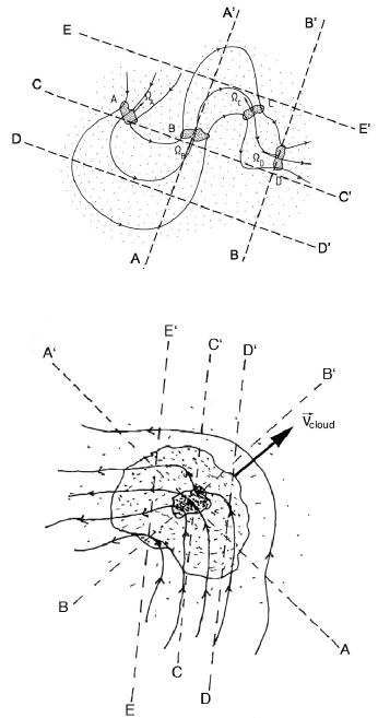
Figure 1: Schematic diagrams: (a, top) A deformed flux tube that has fragmented along its length in a molecular cloud (from Mouschovias & Morton 1985). The deformation can be caused by the relative motion of the fragments. (b, bottom) Deformation of the field lines threading a cloud caused by its motion relative to the surrounding medium. The cloud is shown, for simplicity, to contain only one fragment (or core), in the neighborhood of which the hourglass shape of the field lines had been established during core formation but affected by the cloud’s motion.The dashed lines in both figures represent different lines of sight, whose significance is explained in the text.

Mouschovias & Morton (1985, Fig. 13) had sketched what they regarded as a more realistic field geometry in a molecular cloud in which there are several (in that case four) magnetically connected fragments. That figure is reproduced here as Figure 1a. This configuration can result from relative motion of the fragments (labeled A, B, C, and D) within the cloud, due to the cloud’s mean gravitational field. The motion of a cloud as a whole relative to the intercloud medium will also bend the magnetic field lines in an almost U-shape, as shown in Figure 1b. One can easily visualize lines of sight in Figures 1a and 1b (e.g., the line CC^′) along which a measurement would yield $B_{\rm los,env}>B_{\rm los,core}$, although the actual field strength in the core is greater than that in the envelope as evidenced by the compressed field lines in the core. By contrast, along AA^′, almost the full strength of the core’s magnetic field will be measured, but only a fraction of the envelope’s field strength will be detected. Altogether: (1) An idealization in a theoretical calculation should not be mistaken for a prediction. (2) Observations that may potentially reveal the geometry of the field lines can and should be used as input to build a particular model for the observed cloud (as done in the case of B1 by Crutcher et al. 1994, and for L1544 by Ciolek & Basu 2000). (3) The geometry of the field lines cannot be ignored in analyzing data from observations that measure only one component of the magnetic field (e.g., Zeeman observations) if the purpose is to test a theory or discriminate between alternative theories. The new analysis of the CHT data in § 2.4 accounts for the field geometry suggested by the data themselves.

2.3 Using Data to Calculate a Cloud’s Magnetic Flux

Unlike the CHT analysis, if the data show field reversals, the positive and negative values of the measured $B_{\rm los,env}$ must not be algebraically averaged (which is what the CHT assumption of a single magnetic field value in the envelope imposes on the data) and then multiplied by the plane of the sky area of the envelope in order to obtain its magnetic flux. If the three (perhaps all four) of the observed cloud envelopes exhibited true reversals in the field direction (but see § 2.4 below), that would imply a bent magnetic flux tube threading each cloud. In such a case, only one algebraic sign of the magnetic field (the one corresponding to the greatest absolute values) should be considered in estimating the magnetic flux of the envelope. Figure 2 and its caption clarify this point.

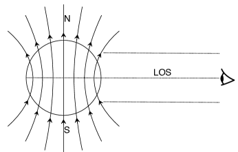
Figure 2: Schematic diagram of a star (e.g., Sun) that has a dipolar magnetic field and is observed (for simplicity) along lines of sight parallel to its equatorial plane. To calculate the magnetic flux threading the star by observing its surface field $B_{\rm surf}$, only the mean value of $B_{\rm surf}$ in either the northern or in the southern hemisphere should be used. If both values are averaged algebraically (as done by CHT), an erroneous flux value of zero will be obtained.

2.4 A Self-Consistent Analysis of the CHT Data

Since both the data and theoretical considerations suggest that $B_{env}$ exhibits spatial variations, we reanalyze the CHT data properly accounting for this effect and thus generalize the relevance of the data to realistic clouds (instead of idealized ones with straight-parallel field lines). High-quality data analyzed in this manner can potentially discriminate between alternative fragmentation theories, instead of just providing geometrical input to theories.

When intrinsic variation of $B_{\rm los}$ in a cloud’s envelope exists, the spread in the observed values is the convolution of the measurement error and of the intrinsic spread of $B_{\rm los}$. To account for spatial variation of $B_{\rm los}$, a likelihood analysis is needed (see Wall & Jenkins 2003; Lyons 1992; Lee 2004). We assume that the “true” $B_{\rm los}$ follows a Gaussian distribution with mean $B_{0}$ and intrinsic spread $\sigma_{0}$. This distribution is then “sampled” with $N$ measurements $B_{j}$, each carrying a (Gaussian) error measurement $\sigma_{j}$.

Table 2: Magnetic Fields and Their Uncertainties (in ${\rm\mu G}$), and Upper Limits on the Envelope Field (in ${\rm\mu G}$) and Ratio $R$

Cloud	$B_{\rm mean}\pm\sigma_{\rm mean}$	$B_{{\rm max}\mathcal{L}}\pm\sigma_{\mathcal{L}}$	$|B_{\rm env}|(\leq 2\sigma)$	$|R|(\leq 2\sigma)$
L1448CO	$0\pm 5$	$-4^{+9}_{-8}$	$27$	$2.0$
B217-2	$+2\pm 4$	$+2^{+7}_{-7}$	$22$	$2.9$
L1544	$+2\pm 3$	$+4^{+10}_{-8}$	$29$	$5.0$
B1	$-8\pm 3$	$-8^{+5}_{-5}$	$20$	$1.1$

Col. 1: The four observed clouds. Col. 2 & 3: Mean field and its uncertainty as given by CHT and by the likelihood data analysis, respectively. Col. 4 & 5: Upper limits on the envelope magnetic field and on the ratio $R$, from the likelihood analysis.

At any specific envelope location, there is a probability $\exp\left[-(B-B_{0})^{2}/2\sigma_{0}^{2}\right]/\sqrt{2\pi}\sigma_{0}$ for the magnetic field to have a true value $B$. If the error of measurement at this same location is $\sigma_{j}$, then the probability of observing a value $B_{j}$ of the field, given that its true value is $B$, is $\exp\left[-(B-B_{j})^{2}/2\sigma_{j}^{2}\right]/\sqrt{2\pi}\sigma_{j}$. However, this is not the only way we could get an observed field value $B_{j}$, since there are many different true values of the field that might yield an observation $B_{j}$ due to measurement errors. To find the total probability for a single observation of $B_{j}$, we integrate over all possible “true” values of the magnetic field at a single location to get (the likelihood for a single observation $B_{j}$ with observational uncertainty $\sigma_{j}$):

$$l_{j}=\int_{-\infty}^{\infty}\!\!\!\!\!\!\!dB\frac{\exp\left[-(B-B_{j})^{2}/(2\sigma_{j}^{2})\right]}{\sqrt{2\pi}\sigma_{j}}\frac{\exp\left[-(B-B_{0})^{2}/(2\sigma_{0}^{2})\right]}{\sqrt{2\pi}\sigma_{0}}\,.$$ (1)

The likelihood $\mathcal{L}$ for $N$ observations of $B_{j}$ with individual uncertainties $\sigma_{j}$ to come from an intrinsic probability distribution with mean $B_{0}$ and spread $\sigma_{0}$ is the product of the individual likelihoods, $\mathcal{L}=\prod_{j=1}^{N}l_{j}$ which, after performing the integration in equation (1) and some algebraic manipulations, yields (see Venters & Pavlidou 2007)

$$\mathcal{L}\left(B_{0},\sigma_{0}\right)=\left(\prod_{j=1}^{N}\frac{1}{\sqrt{\sigma_{0}^{2}+\sigma_{j}^{2}}}\right)\exp\left[-\frac{1}{2}\sum_{j=1}^{N}\frac{(B_{j}-B_{0})^{2}}{\sigma_{0}^{2}+\sigma_{j}^{2}}\right]\,.$$ (2)

Any parameters that are not of direct interest (such as the intrinsic spread $\sigma_{0}$ in this case), can be integrated out of the likelihood. In this way, we can derive the probability distribution of the parameter of interest ($B_{0}$) while still allowing for all possible values in $\sigma_{0}$, rather than arbitrarily demanding that $\sigma_{0}=0$ (as in the CHT analysis). The integrated likelihood is called the marginalized likelihood, $\mathcal{L}_{m}$; this probability distribution can then be used to derive confidence intervals and upper limits where appropriate. The (unnormalized) $\mathcal{L}_{m}$ for the four clouds is shown in Figures 3a - 3d. $\mathcal{L}_{m}$ is derived by numerically integrating equation (2) over $\sigma_{0}$ for different values of $B_{0}$, and is shown as a solid curve in the four figures; the location of the maximum-likelihood estimate for the mean $B_{0}$ is marked by a heavy vertical line in each figure.

The maximum-likelihood estimates and associated uncertainties of $B_{0}$ for the four CHT clouds are shown in Table 2. The uncertainties are systematically greater than those quoted by CHT. The $1\sigma$ uncertainties are represented by the widths of the dark shaded (solid blue) boxes in Figures 3a - 3d. For comparison we show, as cross-hatched boxes, the $1\sigma$ spreads of the values of $B_{0}$ that CHT quote for the same clouds, based on the same data.

Upper limits for $|B_{0}|$ can also be calculated using $\mathcal{L}_{m}$. The $2\sigma$ upper limits for the envelope magnetic field are given in Table 2. (The $2\sigma$ upper limit is that value of $|B_{0}|$ for which a fractional area equivalent to the Gaussian $2\sigma$ ($95.4\%$) is included under the marginalized likelihood curve between $-|B_{0}|$ and $|B_{0}|$. Note that this is not the maximum-likelihood value of $B_{0}$ plus two times the error. In addition, $\mathcal{L}_{m}$ has much longer tails than a gaussian, and hence $1\sigma$, $2\sigma,...$ values do not scale linearly.) The values of $|B_{0}|$ and $-|B_{0}|$ which include between them a fractional area of $2\sigma$ of the marginalized likelihood for the four clouds are marked with heavy down arrows in Figures 3a - 3d.

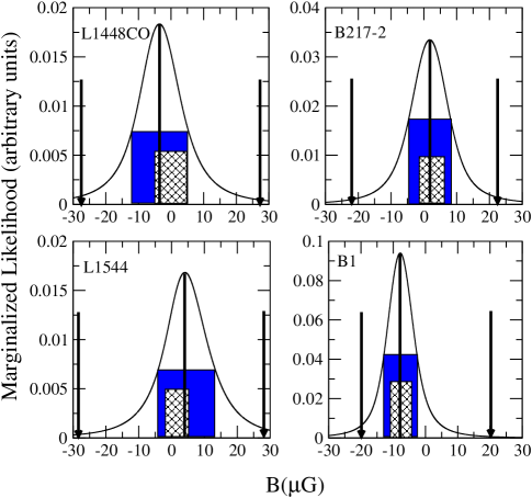
Figure 3: Marginalized likelihood (not normalized, solid curve) for the four cloud envelopes observed by CHT. In each figure: the location of the maximum-likelihood value of $B_{0}$ is marked with a heavy vertical line; the width of the dark shaded (solid blue) box indicates the $1\sigma$ values of $B_{0}$; the width of the cross-hatched box indicates the $1\sigma$ values for $B_{0}$ according to CHT; heavy down arrows mark the $2\sigma$ upper limit on $|B_{0}|$.

To correctly propagate uncertainties onto the derived quantity $R$, we do a full Monte-Carlo calculation to derive the probability distribution for the values of $R$ as follows. We repeat the following experiment $10^{6}$ times: we draw $I_{\rm core}$, $I_{\rm env}$, $\Delta V_{\rm core}$, $\Delta V_{\rm env}$ and $B_{\rm core}$ from gaussian distributions with mean and spread equal to the measurement and uncertainty quoted in CHT; we draw a mean value of $B_{\rm env}$ from the marginalized likelihood of the previous section; we combine all the “mock observations” of these numbers to produce one value of $R$. We use the $10^{6}$ values of $R$ produced in this way to numerically calculate the probability distribution for $R$. We then calculate the $2\sigma$ upper limit on $|R|$ by requiring that the fractional integral of this distribution between $-R$ and $+R$ be $95.4\%$. The $2\sigma$ upper limits for $|R|$ are given in Table 2, last column. These limits are not very strong: $|R|$ is constrained to be smaller than a few, and for no cloud is the upper limit smaller than $1$ $-$ in sharp contrast to the CHT conclusion, that $R$ is in the range 0.02 - 0.42 in the four observed clouds.

In our analysis, we relaxed only one of the CHT assumptions (that of lack of spatial variation of $B_{\rm env}$, which is not consistent with the data). We have retained the implicit assumption of similar orientations of the net ${\mathbf{B}}_{\rm env}$ and ${\mathbf{B}}_{\rm core}$ (vectors), because the data do not suggest any particular relative orientation of the two vectors. A more general analysis that would also relax this assumption would increase the uncertainties on $R$ (although not on $B_{\rm env}$) and would further part from the CHT conclusions.

3 Summary and Conclusion

We have presented a self-consistent analysis of recent OH Zeeman observations by Crutcher et al. (2009), and have shown how such data can be combined in a statistically robust manner to obtain constraints on the mass-to-flux ratio contrast ($R$) between molecular cloud cores and envelopes. Our analysis extends the constraining power of such measurements to realistic clouds, beyond the overly restrictive assumption of straight-parallel field lines in cloud envelopes, adopted by CHT. We have shown that the CHT data are not of good enough quality to constrain the ratio $R$ and thereby test molecular-cloud fragmentation theories: (i) more integration time is needed to reduce measurement errors (now most measurements of $B_{\rm env}$ yield only upper limits); and (ii) more measurements (instead of only four) in each envelope are needed to better constrain the intrinsic spatial variation of $B_{\rm env}$. This kind of observations coupled with the method of data analysis we presented in this Letter has great promise and can lead to significant progress in the field of ISM physics in general and in understanding the role of magnetic fields in molecular-cloud dynamics in particular.

References

- [Ciolek & Basu(2000)] Ciolek, G. E., Basu, S., 2000, ApJ, 529, 925
- [Crutcher 1999] Crutcher, R. M., 1999, ApJ, 520, 706
- [Crutcher et al.(2009)] Crutcher, R. M., Hakobian, N., & Troland, T. H. 2009, ApJ, 692, 844
- [Crutcher et al.(1994)] Crutcher, R. M., Mouschovias, T. Ch., Troland, T. H., Ciolek, G. E., 1994, ApJ, 427, 839
- [Falgarone et al.(2008)] Falgarone, E., Troland, T. H., Crutcher, R. M., Paubert, G., 2008, A&A, 487, 247
- [Fiedler & Mouschovias(1992)] Fiedler, R. A., Mouschovias, T. Ch., 1992, ApJ, 391, 199
- [Fiedler & Mouschovias(1993)] Fiedler, R. A., Mouschovias, T. Ch., 1993, ApJ, 415, 680
- [Heiles & Crutcher(2005)] Heiles, C., Crutcher, R. M., 2005, in Cosmic Magnetic Fields, eds. R. Wielebinski & R. Beck (Berlin: Springer), 137
- [Lee 2004] Lee, P. M., 2004, Bayesian Statistics, Oxford University Press, New York
- [Lunttila et al. 2008] Lunttila, T., Padoan, P., Juvela, M., Nordlund, A. 2008, ApJ, 686, L91
- [1] Lyons, L., 1992, Statistics for Nuclear and Particle Physicists, Cambridge University Press, New York