Asymptotic analysis of the Ponzano-Regge model for handlebodies
Abstract
Using the coherent state techniques developed for the analysis of the EPRL model we give the asymptotic formula for the Ponzano-Regge model amplitude for non-tardis triangulations of handlebodies in the limit of large boundary spins. The formula produces a sum over all possible immersions of the boundary triangulation and its value is given by the cosine of the Regge action evaluated on these. Furthermore the asymptotic scaling registers the existence of flexible immersions. We verify numerically that this formula approximates the 6j-symbol for large spins.
1 Introduction
In [1], Ponzano and Regge gave a formula for the large spin limit of the 6j symbol. It was found to be related to the Regge action for discrete general relativity and with this motivation they constructed the first spin foam model of 3d gravity. Their asymptotic formula was first proved in [2] then more recently using different methods in [3, 4] and the square of the 6j symbol was also studied in the context of relativistic spin networks [5, 6]. The next to leading order approximation was recently considered in [7]. The precise formulation of the full state sum was studied in [8].
In [9, 10], the semiclassical limit of some recent spin foam models [11, 12, 13] was analysed using the coherent state techniques introduced in [13]. In particular the boundary there was formulated in term of coherent tetrahedra. Here we apply the same techniques in the 3d case using coherent triangles and, instead of a single vertex amplitude, we analyze triangulations of arbitrary genus handlebodies. This finally opens up the possibility of a continuum limit and renormalization analysis of the model for this restricted class of 3-manifolds. In particular the resulting formula is well suited for studying the graviton propagator as introduced for Ponzano-Regge in [14].
We begin the paper by describing the formulation of the Ponzano-Regge model in terms of a single spin network diagram dual to the boundary triangulation. We then describe the boundary state choice in detail and proceed to give the asymptotic formula in terms of immersions of the boundary triangulation. The asymptotic scaling of the amplitude has the interesting feature that it registers whether or not there are flexible immersions of the boundary. An explicit example is provided in Steffen’s polyhedron. This analysis sheds light on the general way in which asymptotic behaviour for larger triangulations can emerge from a spin foam model. In particular it does not need to proceed by taking the asymptotics of the individual simplex amplitudes first.
2 The Ponzano-Regge model in terms of coherent states on the boundary
The Ponzano Regge amplitude was originally defined in terms of 6j symbols with a cutoff regularization on the interior vertices. More recently, it was shown in [8] that the cutoff regularization for sums over representations in some cases disallows a 2-3 Pachner move (the Biedenharn-Elliot identity does not hold for a restricted sum over representations.) This meant topological invariance of the partition function can not be proved with Pachner moves in this form. The alternative formulation in terms of delta functions and integrals over regularized with a gauge fixing tree is both finite and invariant under Pachner moves. Another regularization using representations of a quantum group is given by the Turaev-Viro model, however it was also shown in [8] that the limiting procedure that gives the Ponzano-Regge model is only known to exist for so-called non-tardis triangulations - i.e. a triangulation whose edge lengths are restricted to a finite range by the boundary edge lengths. In order to avoid discussing regularization, in this paper we will restrict to only considering these non-tardis triangulations which are by definition finite. Slightly extending the terminology of [8], we will call a manifold a non-tardis manifold if there exists a ‘non-tardis’ triangulation of .
For a 3-manifold with orientable 2-boundary its boundary state space is then given by the possible geometric triangulations of the 2-boundary with half integer edge lengths. The amplitude for such a non-tardis manifold is given in terms of a non-tardis triangulation of that extends the boundary triangulation, and some boundary state :
| (1) |
Here is an edge, a triangle and a tetrahedron of the triangulation of the interior, are half integers labelling the irreps of . The amplitudes and are the spin network evaluation of the theta graph and the planar tetrahedral spin network respectively. These spin networks are the two dimensional duals to the interior triangles and, respectively, to the surface of the tetrahedra in the triangulation. The labelling of the spin network surface duals of the and is given by assigning the associated to each edge to each dual edge that crosses it. Finally is the (super)-dimension of the th irrep in graphical calculus.
In the interior the normalisation and phase of the intertwiners cancels. However, at the boundary these are arbitrary normalisation for each face. This information is in the boundary state which consists of the boundary edge length data and the particular intertwiner chosen at each face.
2.1 Ponzano Regge on the boundary
In some cases it is possible to reformulate the Ponzano-Regge model defined above as a spin network evaluation on the 2-boundary of the manifold. In fact, Ponzano and Regge originally constructed the state sum model such that it agreed with the evaluation of a planar spin network associated to the boundary of a 3-ball. An algorithm to construct a non-tardis interior triangulation given an arbitrary triangulation of the boundary of , was given using recoupling theory by Moussouris in [15]. This algorithm consists of reducing the boundary spin network to a product of 6j symbols (which is always possible for a planar diagram) using the recoupling identity and Schur’s Lemma and then reconstructing the interior triangulation from these 6j symbols. Since the boundary spin network is finite, this procedure gives a manifestly finite definition of the partition function.
In this paper we will extend this result to spin networks on the boundary of handlebodies of arbitrary genus. A non-tardis triangulation of a handlebody of genus can be constructed as follows. Start with a triangulation of the boundary of with distinct pairs of triangles that do not share a common vertex. The boundary of the handlebody can be formed by identifying these triangles and a non-tardis triangulation of the interior is given by applying the Moussouris algorithm. This procedure may result in a degenerate triangulation of the handlebody even if the triangulation of the ball is non-degenerate.
We will begin our analysis by reformulating the amplitude for the 3-ball on a non-tardis triangulation as a spin network on the boundary by a “reverse Moussouris algorithm.” We then describe how this procedure is altered for handlebodies of arbitrary genus. From now on, denotes a handlebody.
Lemma 1.
The Ponzano-Regge amplitude for a non-tardis triangulation of can be expressed in terms of a single spin network evaluation
| (2) |
where ∗ is the two dimensional dual of the surface triangulation with each dual edge labelled with the irrep corresponding to the length of the edge it is dual to, and the spin network is evaluated as the planar projection without crossings, with the intertwiner normalisation given by .
Proof: In order to reexpress the 3-ball with a given triangulation and the amplitude as the spin network evaluation of its boundary we proceed inductively. Note first that a triangulation of given by a single tetrahedron is already of the form we want to put it in: by (1) its amplitude is given exactly by the evaluation of the spin network dual to its boundary 2-geometry with an intertwiner normalisation chosen at each surface triangle. This establishes the base case. We now need to show that the statement remains true when one glues tetrahedra on to a ball amplitude already expressed in this manner, and thus reconstruct arbitrary non-tardis triangulations of the 3-ball. To glue we add the necessary face and edge amplitudes for the new interior faces and edges with the same the normalisation and phase choice of the intertwiners chosen in the boundary state before. These boundary choices will therefore cancel. This is in accordance with the observation above that the phase choice and normalisation on the interior are left arbitrary. A tetrahedron can be glued onto a ball non-degenerately with one or two faces:
-
1.
If we glue one face of the tetrahedron with one face of the ball we create an inner triangle. The PR amplitude of the new ball differs from the old one by a and a tetrahedral net. In the spin network evaluation the vertices of the 3-ball and the tetrahedral amplitude corresponding to the glued face, together with the face amplitude, are the normalized projector on the invariant subspace of the irreps on the edges. As both amplitudes being glued already are invariant we can simply replace them with parallel strands, see Figure 1. This changes the spin network graph being evaluated by changing a vertex to a triangle. This is the dual to the change of the surface triangulation, and the resulting amplitude still satisfies the lemma.
-
2.
If we glue two faces of the tetrahedron onto the ball, we create an inner edge and two inner faces, the PR amplitude changes by adding a tetrahedral net, two thetas and one dimension factor. However, these nets correspond exactly to the symbol for changing the ball amplitude from being connected along the dual of the old boundary to the dual of the new boundary.
| \psfrag{j1}{$j_{1}$}\psfrag{j2}{$j_{2}$}\psfrag{j3}{$j_{3}$}\includegraphics[scale={0.25}]{ballnetwork1} |
\psfrag{j1}{$j_{1}$}\psfrag{j2}{$j_{2}$}\psfrag{j3}{$j_{3}$}\includegraphics[scale={0.25}]{ballnetwork2}
Note that for any non-tardis triangulation of we can always build it up from a single tetrahedron by gluing on one or two faces. Furthermore the two operations described above do not introduce crossings and respect the planar projection chosen.
This establishes that one can express the Ponzano Regge amplitude of an arbitrary triangulation of as a spin network evaluation on its boundary . This proves the lemma .
Consider next the case of a solid torus , which we call . Take a disc such that . For future purposes, note that it intersects a non-contractible loop in . We can now always move this disc by a homotopy that keeps on such that its boundary is the union of at least three edges of the boundary triangulation. Due to triangulation invariance we can then choose a triangulation such that has no internal vertex. We can then cut the Ponzano Regge amplitude along this surface, the resulting space is topologically and we can apply the previous lemma. This yields a ball where two discs on the boundary are glued by identifying edges and using the PR face and edge weights. Call the number of edges that make up . As we chose a disc with no internal vertex, the spin network dual to it has to be an vertex string with one outgoing edge per inner vertex, and two at the end. Together with the face amplitudes this is simply the projector onto the invariant subspace of the irreps on the circle . This projection can then be replaced by a group averaging on the strands dual to :
| (3) |
where is the spin network dual to the surface of the torus with inserted along dual edges crossing . The diagram is defined by first cutting along this circle, choosing the planar no crossing diagram of the graph and then connecting up along the identified edges. See figure 2, and Appendix A for an explicit example.
We can easily generalize this example to arbitrary genus handlebodies. By definition, a handlebody of genus comes equipped with a set of standard cuts that reduce the handlebody to the 3-ball. We call these cuts with an index where is a set of labels for the standard cuts. For later use, note that it is always possible to define a complete set of generators of the homology group such that each is transversal to the cut and does not intersect the other cuts. We can choose an equivalent set of cuts that are related to the standard cuts by boundary preserving homotopy as long as the cuts remain non-intersecting. In particular from now on we will choose the cuts so as to lie on the triangulation. This implies a restriction on the class of triangulations considered as such a choice may not exist for small triangulations.
Now we can state:
Lemma 2.
| (4) |
where is a handlebody, is its triangulated boundary which carries half integer labels on its edges and labels the cuts. Choose a set of cuts that lie on the triangulation. is the spin network evaluation of the dual of the triangulation of the surface, with the links labelled by the half integer lengths of the edges they cross and a inserted on every link that crosses a cut . The spin network is evaluated in the planar projection of the boundary of the cut manifold. That is, with all crossings being due to the links crossing a cut.
Proof: Cutting along the discs reduces it to a 3-ball. The spin network evaluation is defined by taking the planar no crossing representation of the graph cut along the circles and then connecting the identified open ends. If we choose a triangulation that triangulates each disc without internal vertices and reexpress the resulting amplitude as a spin network evaluation, then the gluing of the faces corresponds to a projection onto invariant subspaces. Replace the projection onto the invariant subspace by a group integration and we get the lemma.
Note that due to the intertwining property of the spin network the choice of does not matter, it merely moves the insertion in the intertwiner around.
2.2 Coherent triangles
In order to have a clear geometric picture of the amplitude we will choose the intertwiners in the boundary state by using coherent states [16]. These are the highest weight eigenstates of the normalized Lie algebra elements, that is for the Lie algebra generators and , a coherent state in the representation satisfies:
| (5) |
The parameter describes a choice of representative of the equivalence class of states that correspond to the same . These states transform with a phase under the group elements generated by and the label transforms covariantly under the action of . That is for with corresponding element :
| (6) |
For the asymptotic analysis three further properties will be crucial:
-
•
The representation can be constructed as the symmetric subspace of copies of the fundamental representation. In this picture coherent states decompose into a tensor product of coherent states in the fundamental representation. Consequently the group action factorizes:
(7) -
•
The modulus squared of the Hermitian inner product of coherent states is given by:
(8) -
•
Under the action of the standard antilinear structure on (see [9]) the coherent state changes as:
(9) The antilinear map is given by multiplication by the epsilon tensor in the spin representation followed by complex conjugation. commutes with elements.
Note that given a set of three edge labels there is a non zero intertwiner exactly if they satisfy the triangle inequalities. Therefore there is a set of , unique up to such that . We can then choose our intertwiner in the boundary state as
| (10) |
This state is clearly an invariant state. As we noted that acts covariantly as on the labels this choice is only dependent on an unspecified phase as we left open which eigenstates of we are using. In particular it does not depend on the remaining parity as this acts on the plane of the triangle as an element.
Thus choosing normalized compatible with the boundary spin labels fixes the intertwiner states up to a parity choice and up to a phase. These two data will be fixed by considering the gluing of the boundary.
2.3 Regge state
Let be a set of labels for the boundary faces. Then we label the boundary edges by pairs and call the set of such pairs . Let be an orientation preserving map from the -th triangle on to the plane orthogonal to the north pole of (which we denote ). We choose the orientation in to be the one inherited from by taking to be the outward surface normal. As the boundary of is orientable, we can define where .
The requirement that be orientation preserving implies that the triangles with the edge vectors given by all have the same orientation in . In particular we can require them to have the same orientation as we have chosen for . In particular this implies that we can glue up any two triangles , with a common edge in in an orientation preserving way.
Thus there exists an element such that:
| (11) |
Where is the edge vector of triangle that gets glued to triangle . As in [9], is the Levi-Civita parallel translation from triangle to triangle , according to the bases provided by and . Again, given a choice of spin structure for , a choice of a spin frame for each triangle defines the lift as the parallel translation of the spin connection in these frames.
Next we will describe a canonical choice of phase for the boundary state . From (6), is proportional to . Then we fix the relative phase of the coherent states on the boundary:
| (12) |
We call coherent states with the above relative state choice Regge states, and denote them Their image under the antilinear structure is , and states in the fundamental representation are denoted .
The total boundary state is then given by:
| (13) |
Due to the presence of the antilinear map in the definition of the relative phase the overall ambiguity not fixed by (12) cancels in the overall state. At each triangle we have a sign freedom as adding a sign contributes by the admissibility conditions on intertwiners. This shows that as in [9] the possible lifts of are defined by the spin structures on the boundary, and do not rely on the arbitrary spin frame covering chosen to define the lift.
Finally note that inverting the orientation of would have the same effect as turning the state into .
2.4 The Amplitude
We begin with . To evaluate the spin network defining our amplitude in terms of these coherent intertwiners we choose a particular diagrammatic representation of the planar graph. To obtain the spin network evaluation of this graph we then contract the intertwiners chosen using the epsilon inner product defined in terms of the Hermitian inner product by . Number the triangles in the graph from left to right. We then assume that the coherent intertwiners have been specified with respect to this planar representation of the graph as well. Then we have no crossings in the diagram and we can now explicitly write the contraction of coherent intertwiners as:
| (14) | |||||
Where we have written for .
For general manifolds we need to make sure that, after we have chosen the circles, the dual edges crossing a circle all have the same orientation relative to the circle. This can be done by using a planar representation that has all the glued discs strictly left or right of each other. Call the set of edges not crossing circles and the set of edges crossing circle . The amplitude is then given by
| (15) |
Where is a sign factor incurred in the spin network evaluation when connecting up the glued edges in the spin network evaluation. This can then be written as
| (16) |
with the action given by
| (17) |
Note that the ambiguity in the logarithm of a complex number does not affect the amplitude.
2.5 Symmetries of the action
The action (17) has the following symmetries (up to )
-
•
Continuous. A global rotation acting on each and as and . This represents a rigid motion of the whole manifold.
-
•
Discrete. At each triangle the transformation with leaves a factor . As the admissibility conditions are satisfied on each triangle, this factor equals one. Similarly we have an arbitrary sign on as the edges on which act satisfy the admissibility condition for intertwiners.
This latter symmetry will be used to compensate for the ambiguity of the lifts of to . We can now state the theorem on the asymptotic formula.
2.6 Relation to the standard intertwiner phase choice
The standard choice of phase for an intertwiner, defined by chromatic evaluation [17], gives real numbers for a spin network evaluation. We will now show that with the Regge phase choice the amplitude is real so can only differ from the chromatic evaluation by and a normalisation factor. Note that since the Regge choice has all the orthogonal to , the rotation rotates to and leaves invariant. Under this rotation, the coherent state will transform as
| (18) |
for some phase .
Consider a single term in the amplitude (15), and rewrite it inserting the identity:
| (19) | |||||
where we have defined the transformation , which can be absorbed on the group integration in (15) and the fact that . We have used the Regge phase choice (12) from going from the first to the second line and the fact that the transformations are all in fact in the same subgroup (and hence commute). From going to the second to the third line we have noted that we are acting with opposite rotations on the same state. Hence we get that which is thus real.
3 Asymptotic formula
We wish to study the semiclassical limit of the amplitude . In order to do this, we homogeneously rescale the spin labels by a factor . The corresponding boundary state is given by .
Given a set of boundary data we denote as the set of cut immersions of the polyhedral surface with edge lengths in up to rigid motion.
A cut immersion is an immersion of the manifold obtained from by the trivializing cuts , , i.e. it is an immersion . Furthermore, we require the existence of elements that identify the two sides of the cut, i.e. such that , where and are the elements of the boundary created by the removal of from 444Note that since is transversal to generators of , its removal changes the connectivity of and creates two new boundaries, and . .
Any two cut immersions of are defined to be equivalent, and can be obtained from each other if the cuts are related by a homotopy on the surface. Therefore, different choices of cuts lead to equivalent cut immersions. An example of a cut immersion is given in Figure 3.
Such an immersion is called rigid if every continuous deformation of it requires changing the edge lengths, and flexible otherwise. We denote the subset of rigid immersions . Through every immersion in passes at least one manifold (with dimension ) of immersions that can be continuously deformed into each other. We call these flexifolds and denote them , we denote the set of flexifolds . We then define to be the set of flexifolds in of maximal dimension . With this definition the rigid immersions are a special case of a flexifold with dimension . We assume from now on that the flexifolds do not intersect.
In the limit we have the following theorem:
Theorem 1.
(Asymptotic formula)
-
1.
If is not empty we have that:
(20) The coefficient , the dihedral angle and the phase are independent of . The and the dihedral angle are evaluated on an arbitrary immersion in . It can be shown that these are independent of the cuts. Thus for any particular edge we can evaluate the dihedral angle by moving the cut away from it. is the number of triangles (or equivalently vertices in the set ) and is the number of cutting circles. is the dimension of the flexifolds , and now also contains an integral over the union of flexifolds in .
-
2.
If no immersions in exist the amplitude is exponentially suppressed:
(21)
Note that in the simple case where the boundary data only admits rigid immersions, ie if , then the sum becomes a sum over the rigid immersions and we have that:
| (22) | |||||
since . Since the immersions are now rigid, the coefficient , the dihedral angles and the phase are evaluated on the cut immersion .
4 Proof of the asymptotic formula
We now prove the above theorem. We begin by describing the methods used to give the asymptotic form of the amplitude, this will require finding the so-called stationary and critical points of the action. We can then interpret these points geometrically and give the asymptotic formula. Much of this section is similar to [9] but one dimension lower so the analysis will be as brief as possible.
4.1 Stationary phase
To find the asymptotic form of the amplitude , we will use the complex stationary phase formula [18]. The details of this are recalled below.
Let be a closed manifold of dimension , and let and be smooth, complex valued functions on such that the real part . Consider the function
| (23) |
The Hessian of is the matrix of second derivatives of denoted . For now let us assume that the stationary points are isolated, which, by the Morse lemma is a condition equivalent to the statement that the Hessian is non-degenerate at the critical points; . Such functions are called Morse functions.
In the extended stationary phase, the key role is played by critical points, that is, points , which are not only stationary: but for which as well. So to compute the dominant terms in the asymptotics for large spins, we need to find the stationary points of the action and restrict to those with zero real part. If has no critical points then for large parameter the function decreases faster that any power of . In other words, for all :
| (24) |
If there are isolated critical points, then each critical point contributes to the asymptotics of by a term of order . For large the asymptotic expansion of the integral yields for each critical point
| (25) |
At a critical point, the matrix has a positive definite real part, and the square root of the determinant of this matrix is the unique square root which is continuous on matrices with positive definite real part, and positive on real ones. If admits several isolated critical points with non-degenerate Hessian, we obtain a sum of contributions of the form (25) from each of them.
If there are also degenerate critical points, more care is needed to compute the asymptotics (see eg [19]). Let denote the set of critical points. For the action we will show that is the set of immersions . Note that we cannot a priori assume to be a disjoint union of manifolds as the flexifolds in can intersect. However, here we have restricted ourselves to this case so that the following generalized stationary phase theorem applies.
For a smooth function whose critical set is a disjoint union of closed manifolds555In the literature this is called a Morse-Bott function. A Morse function is the special case where the critical manifolds are zero-dimensional (so the Hessian at critical points is non-degenerate in every direction, i.e., has no kernel)., each critical manifold of dimension , labelled by some on the critical manifold, contributes the following to the asymptotic formula [19]:
| (26) |
where is the restriction of the matrix to the directions normal to with respect to some Riemannian metric on the domain , and is the canonical measure induced on the critical submanifold by the same Riemannian measure on the domain space. This extends to the case where is a manifold-with-boundary.
4.1.1 Critical points
As described above, we must find the points of the action (17) such that as these are the only points that contribute in the limit . First, we introduce some more notation. The action of the elements on the coherent states will produce a new coherent state
| (27) |
We will denote the corresponding rotated three vectors by
| (28) |
where is the element corresponding to .
We will first consider critical points for edges that are not on one of the cutting circles. Using (8), we can see that the real part of the action is given by
| (29) |
This does not depend on the coherent state phases as it is real. Using this formula, we can see that when for all , or explicitly in terms of rotations
| (30) |
The critical points for an edge that crosses a cutting circle differ by the inclusion of the
| (31) |
4.1.2 Stationary points
The stationary points are found by varying the action with respect to each of the group variables . The variation of an group variable and its inverse is
| (32) |
for an arbitrary Lie algebra element . The stationary points are given by and lead to the following equation
| (33) |
where
| (34) |
These equations can then be evaluated at the critical points to give
| (35) |
which is the closure constraint for an immersed triangle.
The stationary phase condition for the variables is the same but in this case we obtain
| (36) |
Which is the closure condition for edges on the circle immersed in . Note that unlike the closure condition for the triangle, this relation involves the as each edge belongs to a different triangle.
If the critical points are not isolated but form a manifold of critical points, then we denote this manifold by
| (37) |
4.2 Geometry
We will now describe how the critical/stationary points can be given a geometric interpretation. We first consider the case where the critical points are isolated.
Theorem 2.
(Geometry) Given a set of boundary data satisfying the closure constraint on each triangle, the solutions to the critical and stationary point equations (30), (31) and (36) correspond to the oriented geometric immersions of a geometric triangulated 2-manifold with boundary obtained by a suitable cutting of the boundary manifold. This immersion is subject to the constraint that a set of exist that map the immersion of to the parity flipped , that is, the immersion of is congruent and oppositely oriented to the immersion of .
The geometric vectors of the immersion are given by
Its orientation the one induced by the vectors on each face.
Conversely, an immersed surface determines a set of and a set of elements .
Proof: Start somewhere on the surface of that is not in a circle. Since has connected boundary, the entire surface is now contractible to this point if cut along the circles. Take the triangle you are on as embedded in and rotate it according to the stationary point equations to . Embed the next triangle and rotate it, according to the stationary point equations it’s edges are now antiparallel to already immersed edges. As they are geometrically glued a translation exists that identifies all its edges with already immersed ones. Thus iteratively the whole immersed surface can be built up and the closure conditions on the cuts now imply that the surface closes up. Finally the stationarity equations on the circles imply that the identifies the circles where we cut the surface.
Conversely given an oriented immersion with the right edge lengths we can choose a set of edge vectors compatible with the orientation on the surface. On each triangle there are two linearly independent edge vectors. The map from these to the corresponding boundary elements defines a rotation in . On the boundary circles we explicitly have elements. The complete set of these solves the critical point equations.
If there is a manifold of dimension of critical points then Theorem 2 holds for each critical point in . Since these critical points lie on a manifold, there is a continuous deformation of the immersed surface that does not change the edge lengths. Hence these critical points reconstruct flexible immersions and we arrive at the flexifolds described in section 3. We will now label the critical manifolds by , where is the flexifold that it describes.
Geometrical interpretation
We will now describe in some more detail the geometric structure of these surfaces. Given an oriented surface in the standard orientation automatically gives us a consistent set of normals . By our choice of boundary data we have automatically ensured that these are given simply by
We can define the dihedral rotation for an oriented surface unambiguously as the rotation around the geometric edge vector that takes to , that is
and
the lift of this rotation can thus be written as
| (38) | |||||
where we require . We then call the dihedral angle. As this definition clearly implies . If we have a surface defining a convex subspace of this definition reduces to the usual definition. In particular the consistent choice of orientation then ensures that we have and for outward facing normals.
On the boundaries of the surface we can also define an analogue of the dihedral rotation by requiring
and
Geometrically this makes sense as it corresponds to the angle obtained by gluing on the two identified boundaries.
Commuting diagram
To fully connect the geometry of these surfaces to the boundary we can relate the dihedral rotation to the gluing of the boundary defined above.
Consider the following diagram which applies to two adjacent triangles that are not on a cutting circle:
| (39) |
Here is the boundary triangle at with edge vectors given by and is the triangle rotated according to its location in the surface, which according to the reconstruction theorem 2 has edge vectors given by . The action of this diagram immediately commutes, as can be seen by acting on and . As an diagram this equation defines a sign that makes it commute. The discrete sign symmetry of the action can be seen as acting on this sign by .
Now, for two triangles whose common edge is on a cutting circle , in the same way we have a commuting diagram as
| (40) |
and additionally have .
We now show that the dihedral rotation is unchanged by moving the cut. Suppose that , in the sense that the edge crosses the cutting circle labelled . Now choose a different, yet homotopic, cutting circle , such that now , but . This corresponds to sliding the cut from one edge of to another, and as any other change in the cut, it will modify wether labels and satisfy (30) or (31). By our orientation convention, we now have
| (41) |
By just looking at the first set of equations above, and comparing it to we have that . This shows that and are equal up to a phase, and by the reconstruction theorem in fact . Hence, comparing the diagrams (39) and (40) we get that moving the cut does not affect the dihedral angle as here defined.
Parity
Given an oriented surface immersed in all surfaces related to it by clearly have the same boundary data. Those related by also have the same dihedral angle as defined above. However if we act by parity we switch the dihedral angle. This is because the two equations defining are invariant under parity, and the dihedral rotation is unchanged. Thus by the definition of the dihedral angle we have
and so .
4.3 The Regge action
Now note that given a geometric surface and associated solution , we can obtain the solution corresponding to the parity flipped surface explicitly. That is, by equation (38) we have that
| (42) |
Acting with by the left of the commuting diagram equations, using the notation if not on a circle and if on, we get
| (43) |
where we have used (42).
It is now straightforward to evaluate the matrix elements in the amplitude. These are of the form . Using the gluing condition this becomes . Finally, by (43) this is just . Thus we have overall that:
| (44) |
Spin Structure
Now we will fix the ambiguity in signs emerging from the spin lifts of the dihedral angle by exploring the discrete sign symmetry in and . Recall that the discrete sign freedom of the action emerged from a different choice of spin frame for each triangle. Now, we show that the discrete sign symmetry related to the cuts corresponds to different choices of spin structures for the manifold . Then, using the fact that is a gauge transform of the connection we can fix the symmetries by adjusting the spin frames and the spin structure such that . Thus we will show that:
Lemma 3.
The signs arising from the spin lift on each face not on the cut obey for some . The signs for a face on the cut, i.e. obey where parametrizes the spin structures of .
Proof. First of all, by (4.2) a lift of the dihedral rotations, , are just a gauge transformation of the . Now recall that are parallel translations on the boundary triangles according to the Levi-Civita connection of the associated metric, with being the parallel translation of the respective spin connection (a lift of to ).
But when the geometry around a vertex is continuously deformed to the flat geometry, the holonomy of a trivial cycle around said vertex has to go to the identity rotation, as opposed to a rotation. This implies that for the holonomy around a vertex through triangles and (which of course consists of a trivial cycle), we have
which implies that locally we must have . The problem now is that if there are non-trivial cycles, i.e. , we may not be able to extend this globally, i.e. may not be globally pure gauge.
In other words, for trivial cycles the lift of the holonomy given by the is fixed to be the same as that given by . But not so for the holonomy of a non-trivial cycle; there exist inequivalent spin structures on a manifold. These have a one-to-one correspondence with the elements of , and so are in number. Hence for a non-trivial cycle, dual to the sequence of triangles crossing the circle , we have
| (45) |
where a is introduced whenever there is an implicit choice of spin structure; i.e. it parametrizes the different spin structures associated with the cut.
We reconcile this case with the one by keeping the form for all the edges that do not lie on a circle, i.e. for any . Then by (45) immediately we must have for , . Since our chosen basis for generates all cycles, we can see that this form of has all the right properties demanded by our equations and accounts for the different spin structures.
Therefore, taking advantage of the discrete sign symmetry, we can choose the spin structure to be compatible with the one chosen for the lift of and thus we will have makes . .
Finally, we obtain that the action evaluated at the critical points is the Regge action for the immersed surface .
| (46) |
For the flexible immersions, the action is the same for all points666This is actually a particular case of the “strong bellows conjecture” that was shown in . on the critical manifold so we evaluate it on an arbitrary immersion in the flexifold.
This concludes the derivation of the Regge action.
4.4 Hessian
The stationary phase formula requires us to calculate the Hessian of the action to determine the weights with which the stationary points contribute to the action. This will be a matrix defined by
| (47) |
Where
| (48) | |||
| (49) | |||
| (50) | |||
| (51) |
The global symmetry of the action implies that there is a redundant integration in . This will cause the determinant of the Hessian to be zero unless it is gauge fixed. To solve this, we make the change of variables for some . This has the effect of removing the variables and the integral gives a volume of which can be normalised to one as it is compact. The remaining Hessian is now a matrix. The submatrix at the critical points, is given by
| (52) |
for the diagonal terms. The off diagonal part is
| (53) |
So one can see that only the off-diagonal elements that represent two neighbouring triangles are non zero. The submatrix will be diagonal since each term in the action only contains one term (ie, each dual edge only crosses one cut.)
| (54) |
The mixed terms will be non zero only for triangles with an edge on the cut
| (55) |
Note that
| (56) |
where we used that on the second equality. By (43) we then have , so if we replace the in with the parity related one we now obtain the complex conjugate:
| (57) | |||||
Thus we can see that the action of parity on the Hessian matrix will also result in complex conjugation when evaluated at the critical points.
4.5 Proof of the formula
We can now evaluate the stationary phase approximation to the amplitude defined in (15). We begin by fixing the symmetries of the action. This can be achieved by taking an arbitrary vertex and dropping the group integration associated to it. As shown in section 4.1.1 the critical point equations are the equations for the immersion of a polyhedral surface with the geometry specified in the boundary data. If a particular immersion is rigid no infinitesimal deformation taking it to another such immersion exists and therefore it is an isolated critical point of the amplitude.
For the isolated critical points in we can explicitly evaluate the stationary phase approximation. Having fixed one group integration we are left with a dimensional integration. The overall scaling of these points is thus . Further we obtain a set of critical points for each immersion from the spin lift of each . Finally the derivatives in the Hessian as defined above are taken with respect to a parametrization of with volume , so we need to rescale by this factor. Using equation (44) and lemma 3 the amplitude itself evaluates to the Regge action of the cut immersion:
Taking all these factors together and using the fact that we know parity related immersions to be the complex conjugate of each other we can approximate the contributions of the isolated critical points to the partition function as:
| (58) | |||||
where is the dihedral angle of the edge in the cut immersion . Since the Hessian matrix changes to its complex conjugate with parity, we can absorb the phase of the determinant into the exponentials and combine the terms
| (59) | |||||
If there are any flexible immersions of the boundary data then there will be a manifold of critical points. Since the critical points extremize the action, it must have the same value on every point of the critical manifold. The Hessian therefore has zero modes along the directions of the flexifold and we must treat the integral as having further symmetries in the neighbourhood of the flexifold. Factoring out these changes the scaling of the contribution of these critical points by , where is the dimension of the flexifold. Therefore these immersions dominate the rigid immersions if they exist, their contribution is given by:
| (60) | |||||
is the dihedral angle of the edge of a particular cut immersion in the flexifold . As the action is constant along the flexifold it does not matter where we evaluate it. is given by
| (61) |
where is the Hessian matrix for the transverse directions which we can not give a general formula for. Combining the exponentials into cosines as above we obtain part one of the main theorem.
Finally, if no immersions of the boundary data exist then there are no solutions to the critical point equations and the stationary phase formula gives that the amplitude is suppressed.
5 Example: The Tetrahedron
Here we apply the above results to the well known case of the asymptotics of the amplitude for a single tetrahedron which, with an appropriate choice of normalisation for the boundary intertwiners, will correspond to the 6j symbol. This is a special case of theorem 1 so the proof is the same as above. In particular, the critical and stationary point equations are the same and the action evaluated at these points reduces to the Regge action for a tetrahedron. Since the asymptotic formula for the tetrahedron is already known, we must verify that our formula agrees with this result. This also provides further evidence that the asymptotic formula for the 4d case derived using the same methods in [9] is correct. We begin by noting that, up to parity, the boundary data of a tetrahedron has only one immersion so the sum in the asymptotic formula disappears.
We will also require an explicit formula for the Hessian matrix in order to perform the numerical calculations. For the tetrahedron, the Hessian is the matrix defined by
| (62) |
The global symmetry of the action implies that there is a redundant integration in . This will cause the determinant of the Hessian to be zero unless it is gauge fixed. To solve this, we make the change of variables for . This has the effect of removing the variables and the integral gives a volume of which can be normalised to one as it is compact. The remaining Hessian is now a matrix which, at the critical points, is given by
| (63) |
for the diagonal terms. The off diagonal part is
| (64) |
5.1 Normalisation and scaling behaviour
We can now compare our theorem with the Ponzano-Regge asymptotic formula for the 6j symbol. The Ponzano-Regge formula is
| (65) |
where is the volume of a geometric tetrahedron with edge lengths and are the dihedral angles. Note that the formula scales as due to the volume term. Currently, our formula for the tetrahedron contains the Regge action but the amplitude, phase term and scaling do not obviously agree with (65). We will first consider the intertwiner normalisation, which will be necessary to obtain the correct scaling behaviour and some numerical factors, and then evaluate the Hessian numerically to check the agreement of the remaining terms. The main drawback of the coherent state approach occurs here as it is very difficult to obtain an analytic formula for the determinant of the Hessian matrix.
5.1.1 Intertwiner normalisation
For the 6j symbol, the three valent intertwiners are normalised by dividing by the square root of the theta spin network. The coherent intertwiners that we replaced these with, however, are not normalised. The normalisation of these intertwiners for the coherent tetrahedron was studied in [13] so we will briefly summarise the results for the case of the coherent triangle.
The normalisation of the coherent intertwiner is given in terms of the three edge vectors of the triangle by the Hermitian inner product
| (66) | |||||
where
| (67) |
This integral can be calculated exactly using [16, 17], the result being
| (68) |
Where , and .
The asymptotics of this intertwiner normalisation can also be found using stationary phase [13]. The stationarity of the action gives the closure condition and the action evaluated on the critical points gives zero.
| (69) | |||||
The additional factor 2 comes from the fact that both and are critical points that give the same contribution to the action. is the Hessian matrix of the action which is given by
| (70) | |||||
We can now normalise our formula such that it agrees with the standard normalisation by dividing by a factor for each triangle .
5.1.2 Numerical calculations
With the intertwiner normalisations included in the asymptotic formula, we obtain
| (74) | |||||
Note that we have the correct scaling behaviour once the additional scaling factors from the intertwiners are included. The normalisation terms are real so do not contribute any additional phase.
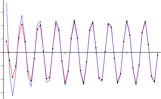
The formula for the equilateral tetrahedron with both the exact and approximate intertwiner normalisation was compared to the 6j symbol and the Ponzano-Regge asymptotic formula using Mathematica in Figure 4. We see that our formula differs from the Ponzano Regge formula for low spins. The only point where our formula differs from Ponzano Regge is in the fact that the Ponzano Regge asymptotics are given in terms of the dihedral angles and volume of the tetrahedron with edge lengths . Therefore the dihedral angles and volume change nontrivially with . A stationary phase approximation extracts only the scaling behaviour with respect to lambda in the asymptotic regime and cannot register this type of low spin behaviour. This agrees as well as the PR formula for larger spins, however the agreement for very low values is not as good - Figure 4.
6 Example: Steffen’s flexible polyhedron
Here we discuss an example for which the second part of theorem 1 is relevant, that is we describe a set of boundary data that admits a flexible immersion. This particular example is taken from a flexible polyhedron with half integer edge lengths consisting of fourteen boundary triangles which was found by K. Steffen [20]. A net for constructing this polyhedron is given in Figure 5 and the corresponding spin network in Figure 6.
Since Steffen’s polyhedron admits a flex in one direction, we know that the flexifold is at least one dimensional. As a polyhedron, it is not allowed to self intersect but there may be other immersions with flexibility in more than one dimension. Applying the asymptotic formula with the same intertwiner normalisation as the tetrahedron in section 5, we would expect the scaling to be .
7 Discussion and Conclusions
7.1 Rigidity of cut immersions
As discussed, the asymptotic formula produces a sum over all possible immersions of the boundary data in , including flexible ones. These flexible immersions scale differently and thus dominate the rigid immersions. The question of whether a particular polyhedron is rigid is a difficult long standing problem in mathematics. A classic result is that convex polyhedra are in fact rigid, however this does not extend to immersions and non convex polyhedra where counter examples, like Steffen’s polyhedron discussed above, are known.
If the boundary data is topologically then a theorem by Steinitz [21] applies that states that any simplicial complex with underlying space homeomorphic to a 2-sphere admits a simplexwise linear embedding into whose image is strictly convex. This embedding will indeed be rigid and we can conclude that for the ball will always be non-empty.
To our knowledge the only more general results on rigidity of immersions are those giving conditions on bar frameworks, that is a graph immersed in , to be generically rigid. A bar framework is considered generic if the coordinates of the vertices are algebraically independent over the rationals, that is, there is no polynomial with rational coefficients that has these coordinates as roots. A graph is generically rigid if all its generic frameworks are. A set of sufficient and neccessary conditions for a graph to be generically rigid are known [22, 23]. Unfortunately this does of course not cover our case with half-integer edge lengths.
Concerning the rigidity of cut immersions, which can be seen as bar frameworks with additional constraints, nothing is known.
7.2 Surface immersions vs interior immersions
With the asymptotic analysis performed above, we explicitly obtain a sum over immersions of the boundary data weighted by the cosine of the Regge action for the immersed surface. Previously, asymptotics of the Ponzano-Regge model for larger triangulations could only be considered by taking the product of the asymptotic formula for each 6j symbol. We now illustrate schematically that, in a simple example, that this is in fact equivalent to the asymptotic formula above.
We will consider the case of two tetrahedra glued along a common triangle and use the boundary normalisation that agrees with the 6j symbol. The partition function then reads
| (75) |
We write the asymptotic formula for the 6j in terms of the Regge action for a tetrahedron
| (76) |
Where several of the factors have been absorbed into the amplitude . Asymptotically, this gives
| (77) | |||||
Where is the parity related tetrahedron and we have used the fact that the Regge action for two tetrahedra becomes
| (78) |
Thus the formula gives a sum over the two different ways of immersing the boundary triangles in , see Figure 7 .
If we now consider larger triangulations, possibly with interior vertices, edges or faces, then the immersed boundary surfaces we obtain are related to immersions of the entire triangulation by adding the immersions of the interior triangulation. Note that the internal vertices can be placed anywhere in which leads to the divergent factors that appear in the Ponzano-Regge state sum for these kind of triangulations. The two parts of the cosine appear because these immersions can be orientation reversing on particular tetrahedra. These will then contribute with negative dihedral angles to the interior action. Thus the integration over possible interior geometries can be split into parts corresponding to particular orientations on the interior tetrahedra. The terms of this sum will then correspond to the sum of terms obtained by multiplying out the sums in the interior cosines. On shell the interior action on these immersions is zero so the overall amplitude only registers the boundary contribution to the action. In particular interior configurations corresponding to different geometries and orientations on the interior, and thus to different terms in the cosine, contribute with the same phase.
7.3 Boundary states
We also note that it is possible to select a particular immersion in the sum by choosing a boundary state peaked around a particular set of dihedral angles, see for example [24, 14, 25]. This boundary state also selects one overall orientation of the immersion which removes the parity related term in the asymptotic formula. For non-rigid immersions, the boundary state would also have the ability to select a particular configuration of the immersed surface which would stop these immersions dominating the integral.
A possible problem with the boundary state is that while it selects an orientation for the boundary, it was not clear if the orientations of the interior tetrahedra behaved consistently. This was considered in [26] and our result also suggests that these do not cause a problem as the asymptotic formula does not register these orientations.
7.4 Conclusions
In this paper we addressed the problem of asymptotics of larger triangulations for the Ponzano-Regge model. By reformulating the partition function as a spin network on the boundary and then rewrote this amplitude using coherent states. While this particular feature will not be available for non topological theories one could expect that in general boundary data will be not suppressed if it can be continued to a solution of the equations of motion on the interior. The asymptotic formula contains a sum over immersions of the boundary data weighted by the cosine of the Regge action. Interestingly, Ponzano and Regge point out in [1] that the different possible immersions corresponding to 3-nj symbols should contribute to the asymptotics but did not obtain a concrete formula. The presented work opens up the possibility to do an exhaustive analysis of the classical limit of the Ponzano Regge model including correlation functions on the boundary. As such it can serve as a toy model and proof of concept for conceptual issues likely to arise in all background independent theories.
Of further interest would be to consider in more detail how the asymptotics obtained here can be obtained from the “product of cosines” picture. In particular to shed light on the issue of causality and orientation in spin foam models.
Interestingly, and unexpectedly, we found that spin networks contain some information about the rigidity properties of surfaces. The scaling properties of a spin network correspond to the maximum dimension of flexibility if the geometry to which it corresponds has any non-rigid immersions.
8 Acknowledgements
RD and FH are funded by EPSRC doctoral grants. We would like to thank John Barrett for discussions and comments on a draft of this paper.
Appendix A Example of the Ponzano-Regge amplitude as a spin network on the boundary of the solid torus
Here we give a simple example of Lemma 2 on the solid torus . A non-tardis (degenerate) triangulation of the solid torus with three tetrahedra is given by
\psfrag{a}{$k_{1}$}\psfrag{b}{$k_{2}$}\psfrag{c}{$k_{3}$}\psfrag{d}{$k_{4}$}\psfrag{e}{$k_{5}$}\psfrag{f}{$k_{6}$}\psfrag{g}{$k_{7}$}\psfrag{h}{$k_{8}$}\psfrag{i}{$k_{9}$}\includegraphics[scale={0.3}]{torus_triangulation}The two triangles with edges are identified. The Ponzano-Regge amplitude is given by
| (79) |
We choose the cutting disc to be the triangle and perform the cut that reduces to the 3-ball. A net for constructing the triangulation on the boundary is given by
\psfrag{a}{$k_{1}$}\psfrag{b}{$k_{2}$}\psfrag{c}{$k_{3}$}\psfrag{d}{$k_{4}$}\psfrag{e}{$k_{5}$}\psfrag{f}{$k_{6}$}\psfrag{g}{$k_{7}$}\psfrag{h}{$k_{8}$}\psfrag{i}{$k_{9}$}\includegraphics[scale={0.25}]{torus_net}The Ponzano-Regge amplitude can be expressed as the following spin network evaluation on the boundary, with a group integral inserted on each of the dual edges that cross .
\psfrag{a}{$k_{1}$}\psfrag{b}{$k_{2}$}\psfrag{c}{$k_{3}$}\psfrag{d}{$k_{4}$}\psfrag{e}{$k_{5}$}\psfrag{f}{$k_{6}$}\psfrag{g}{$k_{7}$}\psfrag{h}{$k_{8}$}\psfrag{i}{$k_{9}$}\psfrag{H}{$h$}\psfrag{int}{$\mathcal{Z}_{PR}(\Psi,\mathbb{T})=\int_{\mathrm{SU}(2)}dh$}\includegraphics[scale={0.35}]{torus_network}Expressing this spin network in terms of 6j symbols gives equation (79).
References
- [1] G. Ponzano and T. Regge, “Semiclassical limit of racah coefficients,” in Spectroscopy and group theoretical methods in physics (F. Block, ed.), pp. 1–58, North Holland, 1968.
- [2] J. Roberts, “Classical 6j-symbols and the tetrahedron,” GEOM.TOPOL., vol. 3, p. 21, 1999.
- [3] R. Gurau, “The ponzano-regge asymptotic of the 6j symbol: an elementary proof,” 2008.
- [4] S. Garoufalidis and R. van der Veen, “Asymptotics of classical spin networks,” 2009, 0902.3113.
- [5] J. W. Barrett and C. M. Steele, “Asymptotics of relativistic spin networks,” Classical and Quantum Gravity, vol. 20, p. 1341, 2003.
- [6] L. Freidel and D. Louapre, “Asymptotics of 6j and 10j symbols,” Class. Quant. Grav., vol. 20, pp. 1267–1294, 2003, hep-th/0209134.
- [7] M. Dupuis and E. R. Livine, “Pushing Further the Asymptotics of the 6j-symbol,” Phys. Rev., vol. D80, p. 024035, 2009, 0905.4188.
- [8] J. W. Barrett and I. Naish-Guzman, “The Ponzano-Regge model,” Class. Quant. Grav., vol. 26, p. 155014, 2009, 0803.3319.
- [9] J. W. Barrett, R. J. Dowdall, W. J. Fairbairn, H. Gomes, and F. Hellmann, “Asymptotic analysis of the EPRL four-simplex amplitude,” 2009, 0902.1170.
- [10] J. W. Barrett, R. J. Dowdall, W. J. Fairbairn, F. Hellmann, and R. Pereira, “Lorentzian spin foam amplitudes: graphical calculus and asymptotics,” 2009, 0907.2440.
- [11] L. Freidel and K. Krasnov, “A New Spin Foam Model for 4d Gravity,” Class. Quant. Grav., vol. 25, p. 125018, 2008, 0708.1595.
- [12] J. Engle, E. Livine, R. Pereira, and C. Rovelli, “LQG vertex with finite Immirzi parameter,” Nucl. Phys., vol. B799, pp. 136–149, 2008, 0711.0146.
- [13] E. R. Livine and S. Speziale, “A new spinfoam vertex for quantum gravity,” Physical Review D, vol. 76, p. 084028, 2007.
- [14] S. Speziale, “Towards the graviton from spinfoams: The 3d toy model,” JHEP, vol. 05, p. 039, 2006, gr-qc/0512102.
- [15] J. Moussouris, Quantum models of space-time based on recoupling theory. PhD thesis, St. Cross College, Oxford, 1983.
- [16] A. Perelomov, Generalized coherent states and their applications. Springer-Verlag, 1986.
- [17] L. H. Kauffman and S. L. Lins, Temperley-Lieb recoupling theory and invariants of 3-manifolds. Princeton University Press, 1994.
- [18] L. Hormander, The analysis of linear partial differential operators I. Springer-Verlag, 1983.
- [19] P. Ramacher, “Singular equivariant asymptotics and the moment map i,” 2009, 0902.1248v1.
- [20] K. Steffen, “A symmetric flexible Connelly sphere with only nine vertices.” See: http://demonstrations.wolfram.com/SteffensFlexiblePolyhedron/ for Mathematica code.
- [21] H. Gluck, “Almost all simply connected surfaces are rigid.,” in Lecture notes in mathematics 438: Geometric Topology, Springer-Verlag, 1975.
- [22] R. Connelly, “Generic global rigidity,” Discrete Comput. Geom., vol. 33, no. 4, pp. 549–563, 2005.
- [23] S. J. Gortler, A. D. Healy, and D. P. Thurston, “Characterizing generic global rigidity,” 2007, 0710.0926.
- [24] C. Rovelli, “Graviton propagator from background-independent quantum gravity,” Phys. Rev. Lett., vol. 97, p. 151301, 2006, gr-qc/0508124.
- [25] E. Bianchi, E. Magliaro, and C. Perini, “LQG propagator from the new spin foams,” 2009, 0905.4082.
- [26] E. Bianchi and A. Satz, “Semiclassical regime of Regge calculus and spin foams,” Nucl. Phys., vol. B808, pp. 546–568, 2009, 0808.1107.