Sparsity and ‘Something Else’: An Approach to Encrypted Image Folding

Abstract

A property of sparse representations in relation to their capacity for information storage is discussed. It is shown that this feature can be used for an application that we term Encrypted Image Folding. The proposed procedure is realizable through any suitable transformation. In particular, in this paper we illustrate the approach by recourse to the Discrete Cosine Transform and a combination of redundant Cosine and Dirac dictionaries. The main advantage of the proposed technique is that both storage and encryption can be achieved simultaneously using simple processing steps.

I Introduction

The problem of reducing the dimensionality of a piece of data without losing the information content is of paramount importance in signal processing. Well-established transforms, from classical Fourier and Cosine Transforms to Wavelets, Wavelet Packets, and Lapped Transforms, just to mention the most popular ones, are usually applied for generating the transformed domain where the processing tasks are realized. Signals amenable to transformation into data sets of smaller cardinality are said to be compressible. Natural images, for instance, provide a typical example of compressible data.

In the last fifteen years emerging techniques for signal representation are addressing the matter by means of highly nonlinear methodologies which decompose the signal into a superposition of vectors, normally called ‘atoms’, selected from a large redundant set called a ‘dictionary’. The representation qualifies to be sparse if the number of atoms for a satisfactory signal approximation is considerably smaller than the dimension of the original data. Available methodologies for highly nonlinear approximations are known as Pursuit Strategies. This comprises Basis Pursuit [1, 2] and Matching-Pursuit-like algorithms, including Orthogonal Matching Pursuit (OMP) and variations of these methods [3, 4, 5, 6, 7, 8, 9, 10]. The other ingredient of highly nonlinear approximations is, of course, the dictionary providing the atoms for the selection. In this respect, Gabor dictionaries have been shown to be useful for image and video processing [11, 12]. Combined dictionaries, arising by merging for instance orthogonal bases, have received consideration in relation to the theoretical analysis of Pursuit Strategies [13, 14, 15, 16, 17]. From a different perspective, other approaches are based on dictionaries learned from large data sets [18, 19].

This communication exploits an inherent side-effect of sparse representations. Since sparsity entails a projection onto a subspace of lower dimensionality, a null space is generated. Extra information can be embedded in such a space and then stably extracted. In particular, we discuss an application involving the null space yielded by the sparse representation of an image, to store part of the image itself in encrypted form. We term this application Encrypted Image Folding (EIF). The main advantage of this proposal, in relation to standard techniques, is that storage and encryption can be achieved simultaneously by means of simple data processing steps. The proposed procedure can be carried out through any suitable transformation. In particular, we consider here the Discrete Cosine Transform (DCT) and a mixed dictionary composed of a Redundant Discrete Cosine (RDC) dictionary and a discrete Dirac Basis (DB). RDC and DB dictionaries are considered separately in [1]. A theoretical discussion with regards to a random collection of elements of a Discrete Sine basis and a DB is presented in [20]. In this letter we would simply like to draw attention to the suitability of mixed dictionaries composed of RDC and DB, for image representation. As far as sparsity is concerned, at the visually acceptable level of 40dB PSNR, they may render a significant improvement in comparison to established fast transforms such as the DCT and Wavelet Transform (WT). An additional advantage of these dictionaries is that Matching Pursuit-like strategies for selecting the atoms can be implemented at a reduced complexity cost by means of the DCT. For these reasons, we illustrate our approach for EIF using a mixed RDC-DB dictionary, in addition to standard the DCT.

The paper is organized as follows: Sec. II motivates the use of a mixed RDC-DB dictionary within the present framework. Sec. III discusses the fact that a sparse representation can be used for embedding information. Based on such a possibility, a scheme for image folding and a simple encryption procedure, fully implementable by data processing, are discussed in Sec.IV. The conclusions are presented in Sec. V.

II Sparse image representation by RDC-DB Dictionaries

Let us start by introducing the dictionaries and methodology which will be used in Section III for illustrating the present approach. Consider the set $D_{a}$ defined as

$$D_{a}=\{\mathbf{v}_{i};\,v_{j,i}=p_{i}\cos(\frac{\pi(2j-1)(i-1)}{2M}),\,j=1,\ldots,N\}_{i=1}^{M},$$

with $p_{i},\,i=1,\ldots,M$ normalization factors and the notation $v_{j,i}$ indicating the component $j$ of vector $\mathbf{v}_{i}\in\mathbb{R}^{N}$. If $M=N$ this set is a Discrete Cosine (DC) orthonormal basis for $\mathbb{R}^{N}$. If $M=2lN$, with $l$ a positive integer, the set is a DC dictionary with redundancy $2l$.

We further consider the set $D_{b}$, which is a discrete DB, also known as standard orthonormal basis i.e.,

$$D_{b}=\{\mathbf{e}_{i}\in\mathbb{R}^{N};\,e_{j,i}=\delta_{i,j},\,j=1,\ldots,N\}_{i=1}^{N},$$

where $\delta_{i,j}=1$ if $i=j$ and zero otherwise. From the joint dictionary $D_{ab}=D_{a}\cup D_{b}$ a redundant dictionary $D$ for $\mathbb{R}^{N\times N}$ is obtained as the Kronecker product $D=D_{ab}\otimes D_{ab}$. We denote by $\mathbf{d}_{n}\in\mathbb{R}^{N\times N},\,n=1,\ldots,J$, where $J=(M+N)^{2}$, the elements of dictionary $D$ and use them to construct the atomic decomposition of an image $\mathbf{I}\in\mathbb{R}^{N\times N}$ as

$$\mathbf{I}^{K}=\sum_{i}^{K}c_{i}^{K}\mathbf{d}_{\ell_{i}}.$$ (1)

The atoms $\mathbf{d}_{\ell_{i}},\,i=1,\ldots,K$ are to be selected from the dictionary $D$ by a Pursuit Strategy. In the examples we give here we have used OMP, which evolves as follows: Setting $\mathbf{R}^{0}=\mathbf{I}$ at iteration $k+1$ the OMP algorithm selects the atom, $\mathbf{d}_{\ell_{k+1}}$ say, as the one maximazing the absolute value of the Frobenius inner products $\langle\mathbf{d}_{i},\mathbf{R}^{k}\rangle_{F},\,i=1,\ldots,J$, i.e.,

$${\ell_{k+1}}=\arg\max\limits_{i=1,\ldots,J}|\langle\mathbf{d}_{i},\mathbf{R}^{k}\rangle_{F}|\,\text{with}\,\mathbf{R}^{k}=\mathbf{I}-\sum_{i=1}^{k}c_{i}^{k}\mathbf{d}_{\ell_{i}}.$$ (2)

The coefficients $c_{i}^{k},\,i=1,\ldots,k$ in (2) are such that the Frobenius norm $\|\mathbf{R}^{k}\|_{F}$ is minimum. Our implementation is based on Gram Schmidt orthonormalization and adaptive biorthogonalization, as proposed in [5]. The complexity is dominated by the calculation of the quantities $\langle\mathbf{d}_{i},\mathbf{R}^{k}\rangle_{F},\,i=1,\ldots,J$ in (2) at each iteration step. For the present dictionaries these quantities can be evaluated by fast DCT. In order to discuss the matter let us re-name the dictionary atoms as follows

$$\text{for }n =1,\ldots,M^{2}$$

$$\mathbf{d}_{n}\to\mathbf{v}_{i}\otimes\mathbf{v}_{j},i=1,\ldots,M,\,j=1,\ldots,M$$

$$\text{for }n =M^{2}+1,\ldots,M^{2}+MN$$

$$\mathbf{d}_{n}\to\mathbf{v}_{i}\otimes\mathbf{e}_{j},i=1,\ldots,M,\,j=1,\ldots,N$$

$$\text{for }n =M^{2}+MN+1,\ldots,M^{2}+2MN$$

$$\mathbf{d}_{n}\to\mathbf{e}_{i}\otimes\mathbf{v}_{j},i=1,\ldots,N,\,j=1,\ldots,M$$

$$\text{for }n =M^{2}+2MN+1,\ldots,J$$

$$\mathbf{d}_{n}\to\mathbf{e}_{i}\otimes\mathbf{e}_{j},i=1,\ldots,N,\,j=1,\ldots,N.$$

Hence, by denoting as $R^{k}(s,r)$ the element $(s,r)$ of matrix $\mathbf{R}^{k}$ and defining $\psi_{j,i}=\cos(\frac{\pi(2j-1)(i-1)}{2M})$, the inner products $\langle\mathbf{d}_{i},\mathbf{R}^{k}\rangle_{F},\,i=1,\ldots,J$ are calculated as

$$\langle\mathbf{v}_{i}\otimes\mathbf{v}_{j},\mathbf{R}^{k}\rangle_{F} =p_{i}p_{j}\sum_{s,r=1}^{N}R^{k}(s,r)\psi_{s,i}\psi_{r,j}$$ (3)

$$\langle\mathbf{v}_{i}\otimes\mathbf{e}_{j},\mathbf{R}^{k}\rangle_{F} =p_{i}\sum_{s=1}^{N}R^{k}(s,j)\psi_{s,i}$$ (4)

$$\langle\mathbf{e}_{i}\otimes\mathbf{v}_{j},\mathbf{R}^{k}\rangle_{F} =p_{j}\sum_{r=1}^{N}R^{k}(i,r)\psi_{r,j}$$ (5)

$$\langle\mathbf{e}_{i}\otimes\mathbf{e}_{j},\mathbf{R}^{k}\rangle_{F} =R^{k}(i,j).$$ (6)

If $M=N$ (3) is the 2D DCT of the residual $\mathbf{R}^{k}$ whilst (4) and (5) are the 1D DCT of the rows and columns of $\mathbf{R}^{k}$, respectively. If $M=2lN$, for some positive integer $l$, the calculations can also be carried out through fast DCT by zero padding. Thus, the complexity required for evaluation of inner products in (2) is $O(M^{2}\log_{2}M)$.

Image	Dictionary	DCT	DWT
Barbara	7.09	4.05	3.92
Boat	6.03	3.63	3.65
Bridge	3.70	2.06	2.20
Film Clip	8.06	4.53	4.81
Jester	6.28	3.6	3.88
Lena	10.06	6.50	6.97
Mandrill	3.32	1.91	1.90
Peppers	7.74	4.36	3.39
Photo (Fig 1)	5.28	3.01	3.15

TABLE I: Sparsity Ratio (for PSNR of 40dB) achieved by the mixed RDC-DB dictionary and that yielded by DCT and DWT.

In order to highlight the capacity of RDC-DB dictionaries to achieve sparse representation of natural images, we use them to represent the popular test images which are listed in the first column of Table I and the photo of Bertrand Russell shown in Fig 1. For the actual processing we divide each image into blocks of $16\times 16$ pixels. The sparsity measure we use is the Sparsity Ratio (SR) defined as

$${\text{SR}}=\frac{\text{total number of pixels}}{\text{total number of coefficients}}.$$

In all the cases the number of coefficients are determined so as to produce a PSNR of 40dB in the image reconstruction and the dictionary is a mixed RDC (redundancy 2) and DB. The results are given in the second column of Table I. For comparison the third column of this table shows results produced by DCT implemented using the same blocking scheme. For further comparison the results produced by the Cohen-Daubechies-Feauveau 9/7 DWT (applied on the whole image at once) are displayed in the last column of Table I. Notice that, while for the fixed PSNR of 40 dB the DCT and DWT yield comparable SR, the corresponding SR obtained by the mixed dictionaries, for all the images, is significantly higher. This motivates the use of RDC-DB dictionaries in the application we are proposing.

III Room for information embedding

Since a sparse representation involves a projection onto a lower dimension subspace, it also creates room for storing ‘something else’. The subspace, say ${\cal{S}}_{K}$, spanned by the $K$-dictionary’s atoms $\{\mathbf{d}_{\ell_{i}}\}_{i=1}^{K}$ rendering a sparse representation of an image is a proper subspace of the image space $\mathbb{R}^{N\times N}$. Thus, denoting by ${\cal{S}}_{K}^{\bot}$ the orthogonal complement of ${\cal{S}}_{K}$ in $\mathbb{R}^{N\times N}$ we have $\mathbb{R}^{N\times N}={\cal{S}}_{K}\oplus^{\bot}{\cal{S}}_{K}^{\bot}$ where $\oplus^{\bot}$ indicates orthogonal sum. Hence, if we take an element $\mathbf{F}\in{\cal{S}}_{K}^{\bot}$ and add it to the image forming $\mathbf{G}=\mathbf{I}+\mathbf{F}$, the image $\mathbf{I}$ can be recovered from $\mathbf{G}$ through the operation

$${P}_{{\cal{S}}_{K}}\mathbf{G}={P}_{{\cal{S}}_{K}}(\mathbf{I}+\mathbf{F})=\mathbf{I},$$ (7)

where ${P}_{{\cal{S}}_{K}}$ is the orthogonal projection matrix, onto the subspace ${\cal{S}}_{K}$. This suggests the possibility of using the sparse representation of an image to embed the image with additional information stored in a matrix $\mathbf{F}\in{\cal{S}}_{K}^{\bot}$. In order to do this, we apply the earlier proposed scheme to embed redundant representations [21], which in this case operates as described below.

Embedding Scheme: Consider that $\mathbf{I}^{K}$ as in (1) is the reconstruction of a sparse representation of an image $\mathbf{I}$. We embed $L=N^{2}-K$ numbers ${{h_{i},\,i=1,\ldots,L}}$ into a matrix $\mathbf{F}\in{\cal{S}}_{K}^{\bot}$ as prescribed below.

• Take an orthonormal basis $\mathbf{u}_{i},\,i=1,\ldots,L$ for ${{\cal{S}}_{K}^{\bot}}$ and form matrix $\mathbf{F}$ as the linear combination

  $$\mathbf{F}=\sum_{i=1}^{L}{h_{i}}\mathbf{u}_{i}.$$ (8)

• Add $\mathbf{F}$ to $\mathbf{I}^{K}$ to obtain $\mathbf{G}=\mathbf{I}^{K}+\mathbf{F}.$

Information Retrieval: Given $\mathbf{G}$ retrieve the numbers ${{h_{i},\,i=1,\ldots,L}}$ as follows.

• Construct an orthogonal projection matrix ${P}_{{\cal{S}}_{K}}$, onto the subspace ${{\cal{S}}_{K}}={\mbox{\rm{span}}}\{\mathbf{d}_{\ell_{i}}\}_{i=1}^{K}$ and extract the image $\tilde{\mathbf{I}}^{K}$ from $\mathbf{G}$ as $\tilde{\mathbf{I}}^{K}={P}_{{\cal{S}}_{K}}\mathbf{G}$.

• From the given $\mathbf{G}$ and the extracted $\tilde{\mathbf{I}}^{K}$ obtain $\mathbf{F}$ as $\mathbf{F}=\mathbf{G}-\tilde{\mathbf{I}}^{K}$. Use $\mathbf{F}$ and the orthonormal basis $\mathbf{u}_{i},\,i=1,\ldots,L$ to retrieve the embedded numbers ${{h_{i},\,i=1,\ldots,L}}$

  $${h_{i}}=\langle\mathbf{u}_{i},\mathbf{F}\rangle_{F},\,i=1,\ldots,L.$$ (9)

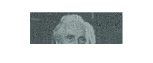
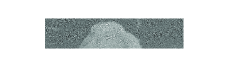
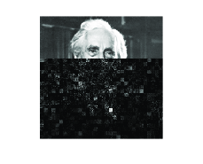
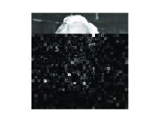
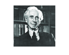
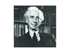
Figure 1: The small pictures at the top are the folded Image by DCT (left) and RDC-DB dictionary (right). The middle pictures are the corresponding unfolded images without knowledge of the private key to initialize the rotation. The bottom pictures are the unfolded images when the correct ${\mathbf{key}}$ is used.

One can encrypt the embedding procedure simply by randomly controlling the order of the orthogonal basis $\mathbf{u}_{i},\,i=1,\ldots,L$ or by applying some random rotation to the basis. An example is given in the next section.

IV Application to Encrypted Image Folding (EIF)

We apply now the above discussed embedding scheme to fold and encrypt an image. For this we process the image by dividing it into $Q$ blocks $\mathbf{I}_{q},\,q=1,\ldots,Q$ of $N_{q}\times N_{q}$ pixels each and compute their sparse representation

$$\mathbf{I}_{q}^{K_{q}}=\sum_{i=1}^{K_{q}}c_{i}^{K_{q}}\mathbf{d}_{q_{\ell_{i}}},\,q=1,\ldots,Q.$$ (10)

We keep a number, $H$, of these block of pixels as hosts for embedding the coefficients of the remaining equations (10). Each host block $\mathbf{I}_{q}^{K_{q}}$ is embedded as follows: Taking $L_{q}=N_{q}^{2}-K_{q}$ of the coefficients to be embedded, we build a block of pixels $\mathbf{F}_{q}$ as in (8) and add it to the host block to obtain $\mathbf{G}_{q}=\mathbf{I}_{q}^{K_{q}}+\mathbf{F}_{q}$. Since the number $H$ of host blocks is the superior integer part of $\frac{Q}{SR}$, as sparsity increases less host blocks are needed to embed the remaining ones. In the example presented here for each host block $q$, with $q=1,\ldots,H$, we have built the orthogonal basis $\mathbf{u}_{i}^{q},\,i=1,\ldots,L_{q}$ (c.f. (8)) by randomly generating matrices $\mathbf{y}_{i}^{q}\in R^{N_{q}\times N_{q}},\,i=1,\ldots,L_{q}$ using a public initialization ${\mathbf{seed}}_{q}$ for the random generator. Through a projection matrix ${P}_{{\cal{S}}_{K_{q}}}$ onto ${\cal{S}}_{K_{q}}={\mbox{\rm{span}}}\{\mathbf{d}_{q_{\ell_{i}}}\}_{i=1}^{K_{q}}$, we compute matrices ${\mathbf{o}}_{i}^{q}\in{\cal{S}}_{K}^{\bot}$ as

$$\mathbf{o}_{i}^{q}=\mathbf{y}_{i}^{q}-P_{{\cal{S}}_{K_{q}}}\mathbf{y}_{i}^{q},\,i=1,\ldots,L_{q}.$$ (11)

Setting an initialization ${\mathbf{key}}$, which remains unknown for an unauthorized user, we apply a random transformation $\Pi_{{\mathbf{key}}}$ on these matrices to obtain a private set of matrices

$$\Pi_{{\mathbf{key}}}:(\mathbf{o}_{i}^{q},\,i=1,\ldots,L_{q})\rightarrow\{\tilde{\mathbf{o}}_{i}^{q}\}_{i=1}^{L_{q}}.$$ (12)

Next, through an orthogonalization procedure $\widehat{\mathbf{Orth}}(\cdot)$ we obtain the orthonormal basis

$$\{\mathbf{u}_{i}^{q}\}_{i=1}^{L_{q}}=\widehat{\mathbf{Orth}}(\tilde{\mathbf{o}}_{i}^{q},\,i=1,\ldots,L_{q}).$$ (13)

that we use for embedding the coefficients of the remaining $Q-H$ blocks.

We illustrate the results on a 8 bit $256\times 256$ photo of Bertrand Russell divided into blocks of $8\times 8$ pixels, using both standard DCT and the RDC-DB dictionary discussed in Sec. II.

The top pictures of Fig. 1 are the folded images using DCT (left) and the RDC-DB dictionary (right). Each block of $8\times 8$ pixels in these figures is the superposition $\mathbf{G}_{q}=\mathbf{I}_{q}^{K_{q}}+\mathbf{F}_{q}$ described above. In both cases the method applied for finding the sparse representation $\mathbf{I}_{q}^{K_{q}}$ is nonlinear, but the DCT case is $O(\overline{K})$ faster than the mixed dictionaries one ($\overline{K}$ being the average number of coefficients per block). Since the SR for the DCT is smaller than the SR for the mixed dictionary, the corresponding folded image is larger. The middle pictures are the unfolded images when an incorrect security ${\mathbf{key}}$ is used. They are obtained as follows: Each block $\mathbf{G}_{q}$ in the top pictures is used to recover the host blocks $\tilde{\mathbf{I}}_{q}^{K_{q}},\,q=1,\ldots,H$ as $\tilde{\mathbf{I}}_{q}^{K_{q}}={P}_{{\cal{S}}_{K_{q}}}\mathbf{G}_{q},\,q=1,\ldots,H$ (top piece of image correctly reconstructed). Subtracting these pixels to the corresponding $\mathbf{G}_{q}$ of the top picture we obtain the pixels $\mathbf{F}_{q}$ which are used to retrieve the embedded coefficients, as in (9) but with matrices $\mathbf{u}_{i}^{q},\,i=1,\ldots,L_{q}$ constructed with an incorrect ${\mathbf{key}}$ (c.f. (13)). As seen in the largest portion of the middle pictures, with these coefficients the image cannot be reconstructed at all. The bottom pictures are obtained in the same way but using the correct ${\mathbf{key}}$. Let us point out that, for reconstructing the image from the coefficients, additional space has to be allowed to store the indices of the atoms in the decomposition (10). This is a requirement of nonlinear approximations for general dictionaries.

Remark 1.

In order to store the folded image at the same bit depth as the original image we need to quantize the blocks of pixels $\mathbf{G}_{q}$ to convert them into integer numbers, which implies some loss of information. However, the quantization step does not prevent us from recovering the coefficients corresponding to the folded pixels with enough accuracy to produce a good representation of those blocks of image. The PSNR of the recovered image $\tilde{\mathbf{I}}^{K}$ in Fig. 1 (after folding it with the RDC-DB dictionary and subsequent rounding) is $40.60$ dB while the PSNR of the original approximation $\mathbf{I}^{K}$ is $40.88$ dB. This implies a relative error due to quantization of $0.68\%$. In further tests, involving forty five 8 bit images of different size and format, the mean value relative error due to quantization was $1.32\%$ with standard deviation $0.57\%$.

Remark 2.

Let us emphasize that since the proposed encryption scheme is based on the orthogonal matrices which define a linear transformation (c.f. (8)), as pointed out in [22] it might be vulnerable to plain text attack. This means that an attacker could discover the matrices $\mathbf{u}_{i}^{q},\,i=1,\ldots,L_{q}$ by collecting, for each block, $L_{q}$-correctly decrypted sets of $L_{q}$ numbers $h_{i,j}^{q}\,i,j=1,\ldots,L_{q}$ encrypted with the identical matrices $\mathbf{u}_{i}^{q},\,i=1,\ldots,L_{q}$. This would indeed allow to pose $L_{q}$ equations of the form (8) and, for invertible systems, disclose the operator used for the encryption. However, the initial step for the construction of this operator involves matrices $\mathbf{y}_{i}^{q},\,i=1,\ldots,L_{q}$ (c.f. (11)) which are randomly generated using a public ${\mathbf{seed}}_{q}$. Hence, for a fixed secret $\mathbf{key}$, it is enough to change the public ${\mathbf{seed}}_{q}$ to avoid $L_{q}$ encryptions with the identical matrices $\mathbf{u}_{i}^{q},\,i=1,\ldots,L$. Thereby, a simple initial setup for the public random initialization of the encryption process prevents the possibility of plain text attack.

V Conclusions

A bonus of sparse image representation has been discussed: the capability for simultaneous storage and encryption by simple processing steps. It was shown that this feature can be used for EIF. The proposed procedure is applicable through any appropriate transformation. The example given here has been produced by a)DCT and b)a combination of RDC and DB dictionaries which is suitable for image processing by blocking. The latter was shown to improve sparsity performance through nonlinear approximation techniques such as OMP. The gain in sparsity also implies that the processing time for the actual folding and unfolding operations is less in the RDC-DB case, as it involves less host blocks to be processed. On the whole, the time spent in both cases is comparable. Using a 2.8Ghz AMD processor with 3GB of RAM, the running time for producing the example of Fig. 1 with MATLAB is (average of ten independent runs) a) 2.39 seconds for DCT and b) 7.05 seconds for RDC-DB. Using a MEX file implementing OMP in C++ the time of b) is reduced to 1.28 seconds. These results suggest that advances in matters of sparse representations may benefit this application.

Acknowledgements

Support from EPSRC, UK, grant (EP$/$D062632$/$1) is acknowledged. We would like to thank Prof Tony Constatinides, from Imperial College, London, for the enjoyable discussions which inspired and further encouraged the application of Image Folding. The software for reproducing the example is available from [23], in section EIFS.

References

- [1] S.S. Chen, D.L. Donoho, and M.A. Saunders. Atomic decomposition by basis pursuit. SIAM Journal on Scientific Computing, 20:33–61, 1998.
- [2] D. Donoho and J. Tanner. Sparse nonegative solution of underdeter-mined linear equations by linear programming. Proceedings of the National Academy of Sciences, 102:94446 – 94451, 2005.
- [3] S. Mallat and Z. Zhang. Matching pursuits with time-frequency dictionaries. IEEE Transactions on Signal Processing, 41:3397–3415, 1993.
- [4] Y.C. Pati, R. Rezaiifar, and P.S. Krishnaprasad. Orthogonal matching pursuit: recursive function approximation with applications to wavelet decomposition. In Proceedings of the 27th Annual Asilomar Conference in Signals, System and Computers, volume 1, pages 40–44, 1993.
- [5] L. Rebollo-Neira and D. Lowe. Optimized orthogonal matching pursuit approach. IEEE Signal Processing Letters, 9:137–140, 2002.
- [6] M. Andrle and L. Rebollo-Neira. A swapping-based refinement of orthogonal matching pursuit strategies. Signal Processing, 86:480–495, 2006.
- [7] P. Jost, P. Vandergheynst and P. Frossard. Tree-Based Pursuit: Algorithm and Properties. IEEE Transactions on Signal Processing, vol 54, pp. 4685-4695, 2006.
- [8] D. Donoho, Y. Tsaig, I. Drori and J-L Starck. Sparse solution of underdetermined linear equations by stagewise orthogonal matching pursuit. Technical Report TR-2006-2, Stanford Statistics Department, 2006
- [9] D. Needell and R. Vershynin. Uniform uncertainty principle and signal recovery via regularized orthogonal matching pursuit. Found. Comput. Math., 2007. DOI: 10.1007/s10208-008-9031-3.
- [10] D. Needell and J.A. Tropp. CoSaMP: Iterative signal recovery from incomplete and inaccurate sampless. Applied and Computational Harmonic Analysis, 26: 301–321, 2009.
- [11] S. Fischer, G. Cristobal, R. Redondo. Sparse overcomplete Gabor wavelet representation based on local competitions. IEEE Transactions on Image Processing 15: 265–272, 2006.
- [12] R. Figueras i Ventura, P. Vandergheynst, P. Frossard Low-rate and flexible image coding with redundant representations IEEE Transactions on Image Processing, 15: 726–739, 2006.
- [13] D. Donoho and X. Huo. Uncertainty principles and ideal atomic decomposition. IEEE Transactions on Information Theory, 47:2845–2862, 2001.
- [14] M. Elad and A.M. Bruckstein, A generalized uncertainty principle and sparse representations of pairs of bases. IEEE Transactions on Information Theory, 48: 2558–2567, 2002.
- [15] A. Feuer and A. Nemirosky, On sparse representation in pairs of bases. IEEE Transactions on Information Theory, 49: 1579–1581, 2003.
- [16] R. Gribonval and M. Nielsen. Sparse representations in unions of bases. IEEE Transactions on Information Theory, 49:3320–3325, 2003.
- [17] J.A. Tropp. Greed is good: algorithmic results for sparse approximation. IEEE Transactions on Information Theory, 50: 2231–2242, 2004.
- [18] B.A. Olshausen and B.J. Field. Emergence of simple-cell receptive field properties by learning a sparse code for natural images. Nature, 381:607–609, 1997.
- [19] M. Elad M. Aharon and A.M. Bruckstein. K-svd: An algorithm for designing of overcomplete dictionaries for sparse representation. IEEE Trans on Signal Processing, 54:4311–4322, 2006.
- [20] J. A. Tropp. On the Linear Independence of Spikes and Sines, Journal of Fourier Analysis and Applications, 14: 838–858,2007.
- [21] J. Miotke and L. Rebollo-Neira. Oversampling of Fourier Coefficients for Hiding Messages, Applied and Computational Harmonic Analysis, 16: 203–207, 2004.
- [22] G. Bhatt, L. Kraus, L. Walters, E. Weber. On hiding messages in oversampled Fourier coefficients. J. Math Anal. Appl. 320: 492–498, 2006.
-
[23]
Highly nonlinear approximations for sparse signal representation.
http://www.nonlinear-approx.info