Probabilistic Weyl laws for quantized tori

Abstract.

For the Toeplitz quantization of complex-valued functions on a $2n$-dimensional torus we prove that the expected number of eigenvalues of small random perturbations of a quantized observable satisfies a natural Weyl law (1.5). In numerical experiments the same Weyl law also holds for “false” eigenvalues created by pseudospectral effects.

1. Introduction and statement of the result

In a series of recent papers Hager-Sjöstrand [13], Sjöstrand [17], and Bordeaux Montrieux-Sjöstrand [3] established almost sure Weyl asymptotics for small random perturbations of non-self-adjoint elliptic operators in semiclassical and high energy régimes. The purpose of this article is to present a related simpler result in a simpler setting of Toeplitz quantization. Our approach is also different: we estimate the counting function of eigenvalues using traces rather than by studying zeros of determinants. As in [13] the singular value decomposition and some slightly exotic symbol classes play a crucial rôle.

Thus we consider a quantization ${\mathcal{C}}^{\infty}(\mathbb{T}^{2n})\ni f\longmapsto f_{N}\in M_{N^{n}}(\mathbb{C})$, where $\mathbb{T}^{2n}$ is a $2n$-dimensional torus, $\mathbb{R}^{2n}/\mathbb{Z}^{2n}$, and $M_{N^{n}}(\mathbb{C})$ are $N^{n}\times N^{n}$ complex matrices. The general procedure will be described in §2 but if $n=1$ and $\mathbb{T}=\mathbb{S}_{x}\times\mathbb{S}_{\xi}$, then

(1.3) $$\begin{gathered}f=f(x)\longmapsto f_{N}\stackrel{{\scriptstyle\rm{def}}}{{=}}{\rm{diag}}\,\left(f(\ell/N)\right)\,,\ \ {\ell=0,\cdots,N-1}\,,\\ g=g(\xi)\longmapsto g_{N}\stackrel{{\scriptstyle\rm{def}}}{{=}}{\mathcal{F}}_{N}^{*}\,{\rm{diag}}\,\left(g(k/N)\right){\mathcal{F}}_{N}\,,\ \ {k=0,\cdots,N-1}\,,\end{gathered}$$

where ${\mathcal{F}}_{N}=(\exp(2\pi ik\ell/N)/\sqrt{N})_{0\leq k,\ell\leq 0,N-1}$, is the discrete Fourier transform.

Let $\omega\mapsto Q_{N}(\omega)$ be the gaussian ensemble of complex random $N^{n}\times N^{n}$ matrices – see §3. With this notation in place we can state our result:

Theorem.  Suppose that $f\in{\mathcal{C}}^{\infty}(\mathbb{T}^{2n})$, and that $\Omega$ is a simply connected open set with a smooth boundary, $\partial\Omega$, such that for all $z$ a neighbourhood of $\partial\Omega$,

(1.4) $${\rm{vol}}_{{\mathbb{T}}^{2n}}\left(\{w\;:\;|f(w)-z|\leq t\}\right)={\mathcal{O}}(t^{\kappa})\,,\ \ 0\leq t\ll 1\,,$$

with $1<\kappa\leq 2$. Then for any $p\geq p_{0}>n+1/2$

(1.5) $$\mathbb{E}_{\omega}\left(|\operatorname{Spec}(f_{N}+N^{-p}Q_{N}(\omega))\cap\Omega|\right)=N^{n}\operatorname{vol}_{\mathbb{T}^{2n}}(f^{-1}(\Omega))+{\mathcal{O}}(N^{n-\beta})\,,$$

for any $\beta<(\kappa-1)/(\kappa+1)$.

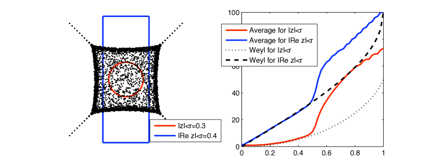
Figure 1. On the left we reproduce [7, Fig.1.2] with two types of regions used for counting added. It represents $\operatorname{Spec}(f_{N}+E)$ where $N=100$, $f(x,\xi)=\cos(2\pi x)+i\cos(2\pi\xi)$ (called the “the Scottish flag operator” in [7]), for a hundred complex random matrices, $E$, of norm $10^{-4}$. On the right we show the counting functions for the two regions, and the corresponding Weyl laws, as functions of $r$. The breakdown of the Weyl law approximation occurs when the norm of the resolvent $(f_{N}-z)^{-1}$, $|z|=r$, or $|\mathop{\rm Re}\nolimits z|=r$, is smaller than $\|E\|^{-1}=10^{4}$. For $\Omega=\{|z|<r\}$, $r<1$, $\kappa=2$ and for $\Omega=\{|\mathop{\rm Re}\nolimits z|<r\}$, $\kappa=3/2$ at four points of $\partial\Omega$ (intersection with the boundary of $f(\mathbb{T})$). For $r=1$, the corners satisfy (1.4) with $\kappa=1$.

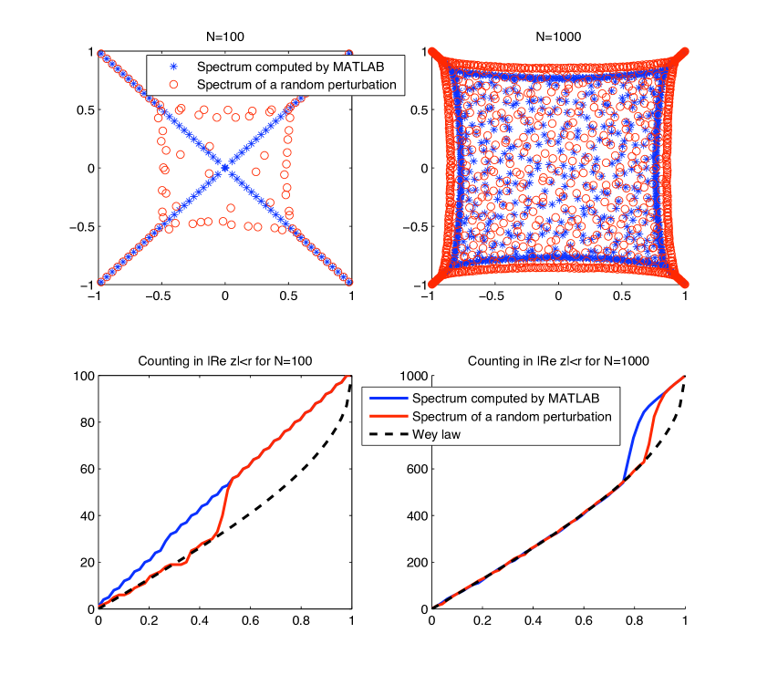
Figure 2. The MATLAB computed spectra of $f_{N}$ for $f(x,\xi)=\cos(2\pi x)+i\cos(2\pi\xi)$. For $N=100$ the computations return the correct eigenvalues following the Scottish flag pattern. For $N=1000$ the actual spectrum of $f_{N}$ still follows the same pattern but the computations return “false eigenvalues” which satisfy the same Weyl law as random perturbations. The plots of the counting function for a single random matrix are very close the Weyl asymptotic even in the case of $N=100$ providing support for the conjecture in §1.

Remark. The theorem applies to more general operators of the form $A(N)=f_{N}+g_{N}/N$, where $g$ may depend on $N$ but all its derivatives are bounded as $N\rightarrow\infty$.

The main point of the probabilistic Weyl law (1.5) is that for most complex-valued functions $f$ the spectrum of $f_{N}$ will not satisfy the Weyl law. Yet, after adding a tiny random perturbation, the spectrum will satisfy it in a probabilistic sense. As illustrated in Fig.2 a tiny perturbation can change the spectrum dramatically, with the density of the resulting eigenvalues asymptotically determined by the original function $f$.

Condition (1.4) with $0<\kappa\leq 2$ appears in the work of Hager-Sjöstrand [13]. Its main rôle here is to control the number of small eigenvalues of $(f_{N}-z)^{*}(f_{N}-z)$, see Proposition 2.9, and that forces us to restrict to the case $\kappa>1$. It is a form of a Łojasiewicz inequality and for real analytic $f$ it always holds for some $\kappa>0$, as can be deduced from a local resolution of singularities – see [1, Sect.4]. Similarly, for $f$ real analytic and such that $f({\mathbb{T}}^{2n})\subset\mathbb{C}$ has a non-empty interior,

$$df\!\!\upharpoonright_{f^{-1}(z)}\neq 0\ \Longrightarrow\ \text{ \eqref{eq:cond} holds with $\kappa>1$.}$$

For $f\in{\mathcal{C}}^{\infty}(\mathbb{T}^{2n})$ we have

$$df\wedge d\bar{f}\!\!\upharpoonright_{f^{-1}(z)}\neq 0\ \Longrightarrow\ \text{ \eqref{eq:cond} holds with $\kappa=2$,}$$

and by the Morse-Sard theorem the condition on the left is valid on a complement of a set of measure $0$ in $\mathbb{C}$. Also,

$$\forall\,w\in f^{-1}(z)\ \ \{f,\bar{f}\}(w)\neq 0\ \text{or}\ \{f,\{f,\bar{f}\}\}(w)\neq 0\ \Longrightarrow\ \text{ \eqref{eq:cond} holds with $\kappa=\frac{3}{2}$,}$$

see [13, Example 12.1]. Here $\{\bullet,\bullet\}$ is the Poisson bracket on $\mathbb{T}^{2n}$ (see (2.32) below).

The significance of the Poisson bracket in this context comes from the following fact:

(1.6) $$\{\mathop{\rm Re}\nolimits f,\mathop{\rm Im}\nolimits f\}(w)<0\,,\ \ z=f(w)\ \Longrightarrow\ \|(f_{N}-z)^{-1}\|>N^{p}/C_{p}\,,\ \forall\,p>0\,,$$

and moreover an approximate eigenvector, $u_{N}$, causing the growth of the resolvent can be microlocalized at $w$ (meaning that for any $g$ vanishing near $w$, $\|g_{N}u_{N}\|_{\ell^{2}}={\mathcal{O}}(N^{-\infty})$, $\|u_{N}\|_{\ell^{2}}=1$, see §2). This is a reinterpretation of a now classical result of Hörmander proved in the context of solvability of partial differential equations – see [8], [20], and references given there. For quantization of ${\mathbb{T}}$ (1.6) was proved in [7], and for general Berezin-Toeplitz quantization of compact symplectic Kähler manifolds, in [5].

The relation (1.6) shows that $\{\bar{f},f\}\neq 0$ implies the instability of the spectrum under small perturbations. In that case the theorem above is most interesting, as shown in Figures 1 and 2. However, as stressed in [3],[13], and [17], the results on Weyl laws for small random perturbations have in themselves nothing to do with spectral instability. For normal operators they do not produce new results compared to the standard semiclassical Weyl laws: the distribution of eigenvalues is not affected by small perturbations and satisfies a Weyl law to start with.

The numerical experiments suggest that much stronger results then our theorem are true. In particular we can formulate the following

Conjecture. Suppose that (1.4) holds for all $z\in\mathbb{C}$ with a fixed $0<\kappa\leq 2$. Define random probability measures:

$$\mu_{N}(\omega)=\frac{1}{N^{n}}\sum_{z\in{\rm{Spec}}\,(f_{N}+N^{-p}R_{N}(\omega))}\delta_{z}\,.$$

Then, almost surely in $\omega$,

$$\mu_{N}(\omega)\longrightarrow f_{*}(\sigma^{n}/n!)\,,\ \ \ N\longrightarrow\infty\,,$$

where $\sigma=\sum_{k=1}^{n}d\xi_{k}\wedge dx_{k}$, $(x,\xi)\in\mathbb{T}^{2n}$, is the symplectic form in $\mathbb{T}^{2n}$.

The result should also hold for more general ensembles than complex Gaussian random matrices. Sjöstrand’s recent paper [17] suggests that random diagonal matrices would be enough to produce the Weyl law-creating perturbations.

Bordeaux Montrieux [2] pointed out to us that by taking singular $f$’s, or $f$’s for which derivatives grow fast in $N$ (corresponding to $\rho=1$ in the $S_{\rho}$ classes described in §2.1), usual Toeplitz matrices fit in this scheme and that numerical experiments indicate the validity of Weyl laws in this case.

Hager [12] indicated how the methods of [13] should apply to the case of Berezin-Toeplitz quantization but that approach did not suggest any simplifications in the method. In this paper we follow the most naïve approach which starts with the following false proof of the theorem:

$$\begin{split}|{\rm{Spec}}\,(f_{N})\cap\Omega|&=\frac{1}{2\pi i}\int_{\partial\Omega}\operatorname{tr}(f_{N}-z)^{-1}dz\\ &\!{\text{``=''}}\,\,N^{n}\frac{1}{2\pi i}\int_{\partial\Omega}\int_{\mathbb{T}^{2n}}(f(w)-z)^{-1}d{\mathcal{L}}(w)dz+o(N^{n})\\ &=N^{n}\int_{\mathbb{T}^{2n}}\left(\frac{1}{2\pi i}\int_{\partial\Omega}(f(w)-z)^{-1}dz\right)d{\mathcal{L}}(w)dz+o(N^{n})\\ &=N^{n}{\rm{vol}}_{\mathbb{T}^{2n}}(f^{-1}(\Omega))+o(N^{n})\,.\end{split}$$

Here we attempted to apply Lemma 2.5 below as if $(f_{N}-z)^{-1}=g_{N}$ for some nice function $g$. As (1.6) shows that is impossible in general. The random perturbation, and taking of expected values, make this argument rigorous. In §4 we show how the first integral split to integrals over small (that is of size $\sim N^{-1/2+\epsilon}$) subintervals of $\partial\Omega$ can be replaced by integrals of invertible operators. That is done using the singular value decomposition (see [18, §3.6] for a simple related example) and facts about random matrices proved in §3. Based on the material reviewed in §2 we further reduce the analysis to that of traces of an inverse of an operator which is a quantization of a slightly exotic function on the torus. Here “slightly exotic” refers to the behaviour of derivatives as $N\rightarrow\infty$. An application of a semiclassical calculus gives the desired trace and concludes the proof.

Except for some facts about the standard semiclassical calculus of pseudodifferential operator recalled in §2.1, the paper is meant to be self-contained. One of the advantages of Toeplitz quantization is the ease with which traces and determinants can be taken, without worries associated with infinite dimensional spaces.

Acknowledgments. We would like to thank Edward Bierstone and Pierre Milman for helpful discussions of Łojasiewicz inequalities, Mark Rudelson for suggestions concerning random matrices, and Stéphane Nonnenmacher for comments on early versions of the paper. The authors gratefully acknowledge the partial support by an MU research leave, and NSF grants DMS 0500267, DMS 0654436. The first author thanks the Mathematics of U.C. Berkeley for its hospitality in spring 2009.

2. Quantization of tori

The Toeplitz quantization of tori, or of more general classes of compact symplectic manifolds, has a long tradition and we refer to [6] for references in the case of tori, and to [4] for the case of compact symplectic Kähler manifolds. We take a lowbrow approach and our presentation which follows [15] is self-contained but assumes the knowledge of standard semiclassical calculus in $\mathbb{R}^{n}$. It is reviewed in §2.1 with detailed references to [9] and [10] provided. To see how this fits in the more general scheme see for instance [5, §4.2].

2.1. Review of pseudodifferential calculus in $\mathbb{R}^{n}$

We first recall from [9, Chapter 7] (see also [10, Chapter 3]) the quantization of functions $a\in S_{\rho}(T^{*}\mathbb{R}^{n})$,

$$S_{\rho}(T^{*}\mathbb{R}^{n})\stackrel{{\scriptstyle\rm{def}}}{{=}}\{a\in{\mathcal{C}}^{\infty}(T^{*}\mathbb{R}^{n})\;:\;\forall\alpha,\beta\in\mathbb{N}^{n},\;|\partial^{\alpha}_{x}\partial_{\xi}^{\beta}a(x,\xi)|\leq C_{\alpha\beta}h^{-(|\alpha|+|\beta|)\rho}\}\,,$$

$$0\leq\rho<\frac{1}{2}\,.$$

To any $a\in{\mathcal{S}}(T^{*}\mathbb{R}^{n})$ we associate its $h$-Weyl quantization, that is the operator $a^{w}(x,hD)$ acting as follows on $\psi\in{\mathcal{S}}(\mathbb{R}^{n})$:

(2.1) $$[a^{w}(x,hD)\,\psi](x)\stackrel{{\scriptstyle\rm{def}}}{{=}}\frac{1}{(2\pi h)^{n}}\int\!\int a\Big{(}\frac{x+y}{2},\xi\Big{)}\,e^{\frac{i}{h}\langle x-y,\xi\rangle}\,\psi(y)\,dy\,d\xi\,.$$

This operator is easily seen to have the following mapping properties

$$a^{w}(x,hD)\;:\;{\mathcal{S}}(\mathbb{R}^{n})\;\longrightarrow\;{\mathcal{S}}(\mathbb{R}^{n})\,,\ \ a^{w}(x,hD)\;:\;{\mathcal{S}}^{\prime}(\mathbb{R}^{n})\;\longrightarrow\;{\mathcal{S}}^{\prime}(\mathbb{R}^{n})\,,$$

see for instance [10, §3.1] for basic properties of the Schwartz space ${\mathcal{S}}$ and [10, §4.3.2] for the mapping properties. It can then be shown [9, Lemma 7.8] that $a\mapsto a^{w}(x,hD)$ can be extended to any $a\in S_{\rho}$, and that the resulting operator has the same mapping properties. Furthermore, $a^{w}(x,hD)$ is a bounded operator on $L^{2}(\mathbb{R}^{n})$. The condition $\rho<1/2$ is crucial for the asymptotic expansion in the the composition formula for pseudodifferential operators. If $a,b\in S_{\rho}$ then

(2.5) $$\begin{gathered}a^{w}(x,hD)\circ b^{w}(x,hD)=c^{w}(x,hD)\,,\ \ c=a\#_{h}b\in S_{\rho}\,,\\ c(x,\xi)\sim\sum_{k=0}^{\infty}\frac{1}{k!}\left(\frac{ih}{2}\sigma(D_{z},D_{w})\right)^{k}a(z)b(w)\!\!\upharpoonright_{z=w=(x,\xi)}\,,\\ \text{where }\sigma(z,w)=\sigma(z_{1},z_{2},w_{1},w_{2})=\langle z_{2},w_{1}\rangle-\langle z_{1},w_{2}\rangle\,.\end{gathered}$$

We note that

$$\frac{1}{k!}\left(\frac{ih}{2}\sigma(D_{z},D_{w})\right)^{k}a(z)b(w)={\mathcal{O}}(h^{k(1-2\rho)})\,,$$

so that the expansion in (2.5) makes sense asymptotically.

It is important to recall the standard way in which the quantization of $S_{\rho}(T^{*}\mathbb{R}^{n})$ reduces to the quantization of

$$S(T^{*}\mathbb{R}^{n})\stackrel{{\scriptstyle\rm{def}}}{{=}}S_{0}(T^{*}\mathbb{R}^{n})\,,$$

with a new semiclassical parameter, $\tilde{h}=h^{1-2\rho}\,.$ Define $(\tilde{x},\tilde{\xi})=(\tilde{h}/h)^{\frac{1}{2}}(x,\xi)$, and a unitary operator on $L^{2}(\mathbb{R}^{n})$:

$$U_{h,\tilde{h}}u(\tilde{x})=(\tilde{h}/h)^{\frac{n}{4}}u((h/\tilde{h})^{\frac{1}{2}}\tilde{x})\,.$$

Then

$$a(x,hD_{x})=U_{h,\tilde{h}}^{-1}\tilde{a}(\tilde{x},\tilde{h}D_{\tilde{x}})U_{h,\tilde{h}}\,,\ \ \tilde{a}(\tilde{x},\tilde{\xi})\stackrel{{\scriptstyle\rm{def}}}{{=}}a((h/\tilde{h})^{\frac{1}{2}}(\tilde{x},\tilde{\xi}))\,.$$

We have

$$a\in S_{\rho}(T^{*}\mathbb{R}^{n})\ \Longleftrightarrow\ \tilde{a}\in S(T^{*}\mathbb{R}^{n})\,.$$

One simple application of this rescaling is a version of the semiclassical Beals Lemma [9, Chapter 8] (see also [10, §8.6]):

(2.8) $$\begin{gathered}A=a^{w}(x,hD)\,,\ \ a\in S_{\rho}(T^{*}\mathbb{R}^{n})\ \Longleftrightarrow\ {\rm{ad}}\,_{\ell^{w}_{1}}\circ\cdots{\rm{ad}}\,_{\ell^{w}_{N}}A={\mathcal{O}}_{L^{2}\rightarrow L^{2}}(h^{N(1-\rho)})\,,\\ \text{for any sequence $\{\ell_{j}\}_{j=1}^{N}$ of linear functions on $T^{*}\mathbb{R}^{n}$}\end{gathered}$$

The composition formula (2.5) holds also for operators in more general symbol classes. For reasons which should become clear below, we will discuss it only for the $\tilde{h}$-quantization with $\rho=0$. First we need to recall the definition of an order function: ${\tilde{m}}={\tilde{m}}({\tilde{x}},{\tilde{\xi}})$ is an order function if there exist $C$ and $M$ such that for all $({\tilde{x}},{\tilde{\xi}})$ and $({\tilde{x}}^{\prime},{\tilde{\xi}}^{\prime})$, we have

$$m({\tilde{x}},{\tilde{\xi}})\leq Cm({\tilde{x}}^{\prime},{\tilde{\xi}}^{\prime})(1+d_{\mathbb{R}^{2n}}(({\tilde{x}},{\tilde{\xi}}),({\tilde{x}}^{\prime},{\tilde{\xi}}^{\prime})))^{M}\,.$$

We then say that $\tilde{a}\in S({\tilde{m}})$ if for all $\alpha$, $|\partial^{\alpha}_{{\tilde{x}},{\tilde{\xi}}}\tilde{a}({\tilde{x}},{\tilde{\xi}})|\leq C_{\alpha}{\tilde{m}}({\tilde{x}},{\tilde{\xi}})$. If ${\tilde{m}}_{1}$ and ${\tilde{m}}_{2}$ are two order functions and $\tilde{a}\in S({\tilde{m}}_{1})$, $b\in S({\tilde{m}}_{2})$ then $\tilde{a}({\tilde{x}},{\tilde{h}}D)\circ\tilde{b}({\tilde{x}},{\tilde{h}}D)=\tilde{c}({\tilde{x}},{\tilde{h}}D)$, $\tilde{c}\in S({\tilde{m}}_{1}{\tilde{m}}_{2})$, and the asymptotic expansion (2.5) is valid in $S({\tilde{m}}_{1}{\tilde{m}}_{2})$.

This has a standard application which will be crucial in §5:

(2.11) $$\begin{gathered}\tilde{a}\in S({\tilde{m}})\,,\ \forall\,({\tilde{x}},{\tilde{\xi}})\,,\ \ |a({\tilde{x}},{\tilde{\xi}})|\geq{\tilde{m}}({\tilde{x}},{\tilde{\xi}})\ \Longrightarrow\\ \exists\,{\tilde{h}}_{0}\,\forall\,0<{\tilde{h}}<{\tilde{h}}_{0}\,,\ \ \tilde{a}^{w}({\tilde{x}},{\tilde{h}}D)^{-1}=\tilde{b}^{w}({\tilde{x}},{\tilde{h}}D)\,,\ \ b\in S(1/{\tilde{m}})\,,\ \ \end{gathered}$$

see for instance [10, §4.5,§8.6].

The reason that we presented the order functions on the ${\tilde{h}}$-side is motivated by the fact that we need the rescaling of these order functions on the ${\tilde{h}}$-side: we say that $m=m(x,\xi)$ is an $h^{\rho}$-order function if there exist $C$ and $M$ such that for all $(x,\xi)$ and $(x^{\prime},\xi^{\prime})$, we have

(2.12) $$m(x,\xi)\leq Cm(x^{\prime},\xi^{\prime})(1+d_{\mathbb{R}^{2n}}(h^{-\rho}(x,\xi),h^{-\rho}(x^{\prime},\xi^{\prime})))^{M}\,,$$

which means that $\tilde{m}({\tilde{x}},{\tilde{\xi}})\stackrel{{\scriptstyle\rm{def}}}{{=}}m(h^{\rho}{\tilde{x}},h^{\rho}{\tilde{\xi}})$ is a standard order function defined above. The symbol class is defined analogously, $a\in S_{\rho}(m)$ if $\partial^{\alpha}a={\mathcal{O}}(h^{-|\alpha|\rho}m)$. By the rescaling argument the ellipticity statement (2.11) is still applicable if $\rho<1/2$.

The following $h^{\rho}$-order function coming from [13, §4] will be essential to our arguments here, and in §5 (Lemma 2.6):

Lemma 2.1.

For $a\in S(T^{*}\mathbb{R}^{n})$

$$m(x,\xi)\stackrel{{\scriptstyle\rm{def}}}{{=}}|a(x,\xi)|^{2}+h^{2\rho}\,,\ \ \ 0\leq\rho<\frac{1}{2}\,,$$

is an $h^{2\rho}$-order function in the sense of definition (2.12). In addition, for $\psi\in{\mathcal{C}}^{\infty}_{\rm{c}}(\mathbb{R};[0,1])$ equal to $1$ on $[-1,1]$,

(2.13) $$\left(|a(x,\xi)|^{2}+h^{2\rho}\psi\left(\frac{|a(x,\xi)|^{2}}{h^{2\rho}}\right)\right)^{\pm 1}\in S_{\rho}(m^{\pm 1})\,.$$

Proof.

This follows from the arguments in [13, §4] but for the reader’s convenience we present an adapted version. We will use the notation $(\tilde{x},\tilde{\xi})$ introduced above, with ${\tilde{h}}=h^{1-2\rho}$. Let us put $F({\tilde{x}},{\tilde{\xi}})\stackrel{{\scriptstyle\rm{def}}}{{=}}|a(x,\xi)|^{2}$, so that $m(x,\xi)=h^{2\rho}{\tilde{m}}({\tilde{x}},{\tilde{\xi}})$ , where

$$\widetilde{m}({\tilde{x}},{\tilde{\xi}})\stackrel{{\scriptstyle\rm{def}}}{{=}}h^{-2\rho}F({\tilde{x}},{\tilde{\xi}})+1\geq 1\,.$$

To prove (2.12) we need

(2.14) $$\widetilde{m}(w)\leq C{\widetilde{m}(w^{\prime})}(1+d_{\mathbb{R}^{2n}}(w,w^{\prime}))^{M}\,,$$

For $|\beta|=1$, $\partial^{\beta}F={\mathcal{O}}(h^{\rho}\sqrt{F})$ and hence

$$\partial^{\beta}\widetilde{m}=\frac{1}{h^{2\rho}}\partial^{\beta}F={\mathcal{O}}(h^{-\rho}\sqrt{F})={\mathcal{O}}(\sqrt{\widetilde{m}})\,.$$

For $|\beta|=2$, $\partial^{\beta}F={\mathcal{O}}(h^{2\rho})$, and hence $\partial^{\beta}{\tilde{m}}={\mathcal{O}}(1)$. By Taylor’s formula,

$$\begin{split}\widetilde{m}(w^{\prime})&\leq\widetilde{m}(w)+C\sqrt{\widetilde{m}(w)}d_{\mathbb{R}^{2n}}(w,w^{\prime})+Cd_{\mathbb{R}^{n}}(w,w^{\prime})^{2}\\ &\leq C(1+\widetilde{m}(w))(1+d_{\mathbb{R}^{2n}}(w,w^{\prime}))^{2}\,.\end{split}$$

As $\widetilde{m}\geq 1$ this proves (2.14) with $M=2$, and consequently the first part of the lemma.

For the second part we observe that $\psi(|a|^{2}/h^{2\rho})\in S_{\rho}(1)$ and hence $h^{2\rho}\psi(|a|^{2}/h^{2\rho})\in S_{\rho}(m)$. This means that we already have the $+$ case of (2.13). But,

$$|a(x,\xi)|^{2}+h^{2\rho}\psi\left({|a(x,\xi)|^{2}}/{h^{2\rho}}\right)\geq m(x,\xi)/2\,,$$

and the $-$ case follows. ∎

We remark that by introducing $\tilde{h}$ as a small, eventually fixed, parameter, we can include the case of $\rho=1/2$ – see for instance [19, §3.3]. That type of calculus is used in [13].

The last item in this review is a slightly non-standard functional calculus lemma:

Lemma 2.2.

Suppose that $a\in S_{0}(T^{*}\mathbb{R}^{n})$, $0\leq\rho<1/2$, and that $\psi\in{\mathcal{C}}^{\infty}_{\rm{c}}(\mathbb{R})$. Then

(2.18) $$\begin{gathered}\psi\left(a^{w}(x,hD)a^{w}(x,hD)^{*}/h^{2\rho}\right)=q^{w}(x,hD)\,,\ \ q\in S_{\rho}(T^{*}\mathbb{R}^{n})\,,\\ q=q_{0}+h^{1-2\rho}q_{1}+{\mathcal{O}}_{S}(h^{\infty})\,,\ \ q_{j}\in S_{\rho}\,,\ \ q_{0}(x,\xi)=\psi(|a(x,\xi))|^{2}/h^{2\rho})\,,\\ q_{1}(x,\xi)=\widetilde{\psi}(|a(x,\xi)|^{2}/h^{2\rho})\widetilde{q}_{1}(x,\xi)\,,\ \ \widetilde{q}_{1}\in S_{\rho}\,,\ \ \widetilde{\psi}\in{\mathcal{C}}^{\infty}_{\rm{c}}(\mathbb{R})\,,\ \ \widetilde{\psi}\!\!\upharpoonright_{{\rm{supp}}\,\psi}\equiv 1\,.\end{gathered}$$

Proof.

This is a simpler version of [13, Proposition 4.1] which follows the approach to functional calculus of pseudodifferential operators based on the Helffer-Sjöstrand formula for a function of a selfadjoint operator $A$:

(2.19) $$\psi(A)=\frac{1}{\pi}\int_{\mathbb{C}}(z-A)^{-1}\partial_{\bar{z}}\tilde{\psi}(z)d{\mathcal{L}}(z)\,,\ \ \psi\in{\mathcal{C}}^{\infty}_{\rm{c}}(\mathbb{R})\,,$$

where $\tilde{\psi}\in{\mathcal{C}}^{\infty}_{\rm{c}}(\mathbb{C})$ is an almost analytic extension of $\psi$, $\tilde{\psi}\!\!\upharpoonright_{\mathbb{R}}=\psi$ and $\partial_{\bar{z}}\tilde{\psi}={\mathcal{O}}(|\mathop{\rm Im}\nolimits z|^{\infty})$ – see [9, Chapter 8] and references given there. The reduction to the case given in [9, Theorem 8.7] proceeds as follows: the operator $a^{w}(x,hD)a^{w}(x,hD)^{*}/h^{2\rho}=b^{w}(x,hD)$, where $b\in S_{\rho}(m_{1})$, where $m_{1}$ is an $h^{\rho}$-order function given by $h^{-2\rho}m$, where $m$ is given in Lemma 2.1. By the rescaling argument above, which gives a reduction to the case of the calculus with $\tilde{h}=h^{1-2\rho}$, we can apply [9, Theorem 8.7] which gives that $\psi(a^{w}(x,hD)a^{w}(x,hD)^{*}/h^{2\rho})=g^{w}(x,hD)$, where $g\in S_{\rho}(m_{1}^{-1})\subset S_{\rho}(1)$. The symbolic expansion presented in [9, Chapter 7] complete the proof. ∎

2.2. Quantum space associated to ${\mathbb{T}}^{2n}$

To define this finite dimensional space we fix our notation for the Fourier transform on ${\mathcal{S}}^{\prime}(\mathbb{R}^{n})$:

$${\mathcal{F}}_{h}u(\xi)\stackrel{{\scriptstyle\rm{def}}}{{=}}\frac{1}{(2\pi h)^{n/2}}\int u(x)\,e^{-\frac{i}{h}\langle x,\xi\rangle}\,dx\,,\qquad{\mathcal{F}}_{h}^{*}={\mathcal{F}}_{h}^{-1}\,,$$

and as usual in quantum mechanics, ${\mathcal{F}}_{h}u(\xi)$ is the “momentum representation” of the state $u$. To find the space of states we consider distributions $u\in{\mathcal{S}}^{\prime}(\mathbb{R}^{n})$ which are periodic in both position and momentum:

(2.20) $$u(x+\ell)=u(x)\,,\qquad{\mathcal{F}}_{h}u(\xi+\ell)={\mathcal{F}}_{h}u(\xi)\,,$$

see [15, §4.1] and references given there for more general spaces with different Bloch angles. Let us denote by ${\mathcal{H}}_{h}^{n}$ the space of distributions satisfying (2.20). The following lemma is easy to prove.

Lemma 2.3.

${\mathcal{H}}_{h}^{n}\neq\{0\}$ if and only if $h=(2\pi N)^{-1}$ for some positive integer $N$, in which case $\dim{\mathcal{H}}_{h}^{n}=N^{n}$ and

(2.21) $${\mathcal{H}}_{h}^{n}={\rm{span}}\left\{\,\frac{1}{\sqrt{N^{n}}}\sum_{\ell\in\mathbb{Z}^{n}}\delta(x-\ell-j/N)\;:\;j\in(\mathbb{Z}/N\mathbb{Z})^{n}\,\right\}\,.$$

For $h=(2\pi N)^{-1}$, the Fourier transform ${\mathcal{F}}_{h}$ maps ${\mathcal{H}}_{h}^{n}$ to itself. In the above basis, it is represented by the discrete Fourier transform

(2.22) $$({\mathcal{F}}_{N})_{j,j^{\prime}}=\frac{e^{-2i\pi\langle j,j^{\prime}\rangle/N}}{N^{n/2}}\,,\quad j,j^{\prime}\in(\mathbb{Z}/N\mathbb{Z})^{n}\,.$$

The Hilbert space structure on ${\mathcal{H}}_{h}$ will be determined (up to a constant) once we define the quantization procedure. That will be done by demanding that real functions are quantized into self-adjoint operators.

2.3. Quantization of ${\mathcal{C}}^{\infty}({\mathbb{T}}^{2n})$.

The definition (2.1) immediately shows that for $f\in{\mathcal{C}}^{\infty}$ satisfying

$$\forall\,\ell,m,\in\mathbb{Z}^{n}\,,\ \ \ f(x+\ell,\xi+m)=f(x,\xi)\ \Longrightarrow\ f^{w}(x,hD)\;:\;{\mathcal{H}}_{h}^{n}\longrightarrow{\mathcal{H}}_{h}^{n}\,,$$

where we consider ${\mathcal{H}}_{h}^{n}\subset{\mathcal{S}}^{\prime}(\mathbb{R}^{n})$. Identifying a function $f\in{\mathcal{C}}^{\infty}({\mathbb{T}}^{2n})$ with a periodic function on $\mathbb{R}^{2n}$, we define

$$f_{N}=f^{w}(x,hD)\!\!\upharpoonright_{{\mathcal{H}}_{h}^{n}}\,,\ \ h=\frac{1}{2\pi N}\,,\ \ \ {\mathcal{C}}^{\infty}({\mathbb{T}}^{2n})\ni f\;\longmapsto\;f_{N}\in{\mathcal{L}}({\mathcal{H}}_{h}^{n},{\mathcal{H}}_{h}^{n})\,,$$

and we remark that $1_{N}=Id_{{\mathcal{H}}_{h}^{n}}$.

The composition formula from §2.1 applies since $a,b\in{\mathcal{C}}^{\infty}({\mathbb{T}}^{2n})$ can be identified with periodic functions on $\mathbb{R}^{2n}\simeq T^{*}\mathbb{R}^{n}$ and

(2.23) $$a_{N}\circ b_{N}=c_{N}\,,\ \ c=a\#_{h}b\,,\ \ h=\frac{1}{2\pi N}\,,$$

where $a\#_{h}b$ is as in (2.5). This means that we simply use the standard pseudodifferential calculus but act on a very special finite dimensional space.

The Hilbert space structure on ${\mathcal{H}}_{h}^{n}$ is determined by the following simple result [15, Lemma 4.3] which we recall below.

Lemma 2.4.

There exists a unique (up to a multiplicative constant) Hilbert structure on ${\mathcal{H}}_{h}^{n}$ for which all $f_{N}\;:\;{\mathcal{H}}_{h}^{n}\;\rightarrow\;{\mathcal{H}}_{h}^{n}$ with $f\in{\mathcal{C}}^{\infty}({\mathbb{T}}^{2n};\mathbb{R})$ are self-adjoint. One can choose the constant so that the basis in (2.21) is orthonormal. This implies that the Fourier transform on ${\mathcal{H}}_{h}^{n}$ (represented by the unitary matrix (2.22)) is unitary.

Proof.

Let $\langle\bullet,\bullet\rangle_{0}$ be the inner product for which the basis in (2.21) is orthonormal, and put

$$Q_{j}\stackrel{{\scriptstyle\rm{def}}}{{=}}\frac{1}{\sqrt{N^{n}}}\sum_{\ell\in\mathbb{Z}^{n}}\delta(x-\ell-j/N)\;:\;j\in(\mathbb{Z}/N\mathbb{Z})^{n}.$$

We write the operator $f^{w}(x,hD)$ on ${\mathcal{H}}_{h}^{n}$ explicitly in that basis using the Fourier expansion of its symbol:

$$f(x,\xi)=\sum_{\ell,m\in\mathbb{Z}^{n}}\hat{f}(\ell,m)\,e^{2\pi i(\langle\ell,x\rangle+\langle m,\xi\rangle)}\,.$$

For that let $L_{\ell,m}(x,\xi)=\langle\ell,x\rangle+\langle m,\xi\rangle$, so that

$$f^{w}(x,hD)=\sum_{\ell,m\in\mathbb{Z}^{n}}\hat{f}(\ell,m)\,\exp(2\pi iL^{w}_{\ell,m}(x,hD))\,.$$

We also check that

$$\exp\big{(}2\pi iL^{w}_{\ell,m}(x,hD)\big{)}\,Q_{j}=\exp({\pi i}(2\langle j,\ell\rangle-\langle m,\ell\rangle)/N)\,Q_{j-m}\,,$$

(note that $j\in(\mathbb{Z}/N\mathbb{Z})^{n}$ and $j-m$ is meant $\mod N$) and consequently,

$$f_{N}(Q_{j})=\sum_{m\in\mathbb{Z}^{n}/(N\mathbb{Z})^{n}}F_{mj}\,Q_{m}\,,$$

$$F_{mj}=\sum_{\ell,r\in\mathbb{Z}^{n}}\hat{f}(\ell,j-m-rN)(-1)^{\langle r,\ell\rangle}\,\exp({\pi i}\,\langle j+m,\ell\rangle/N)\,.$$

Since

$$\begin{split}\bar{F}_{jm}&=\sum_{\ell,r\in\mathbb{Z}^{n}}\hat{\bar{f}}(-\ell,j-m+rN)(-1)^{\langle r,\ell\rangle}\,\exp(-{\pi i}\,\langle j+m,\ell\rangle/N)\\ &=\sum_{\ell,r\in\mathbb{Z}^{n}}\hat{\bar{f}}(\ell,j-m-rN)(-1)^{\langle r,\ell\rangle}\,\exp({\pi i}\,\langle j+m,\ell\rangle/N)\,,\end{split}$$

we see that for real $f$, $f=\bar{f}$, $F_{jm}=\bar{F}_{mj}$. This means that $f^{w}(x,hD)$ is self-adjoint for the inner product $\langle\bullet,\bullet\rangle_{0}$. We also see that the map $f\mapsto(F_{jm})_{j,m\in(\mathbb{Z}/N\mathbb{Z})^{n}}$ is onto, from ${\mathcal{C}}^{\infty}({\mathbb{T}}^{2n};\mathbb{R})$ to the space of Hermitian matrices.

Any other metric on ${\mathcal{H}}_{h}^{n}$ could be written as $\langle u,v\rangle=\langle Bu,v\rangle_{0}=\langle u,Bv\rangle_{0}$. If $\langle f_{N}u,v\rangle=\langle u,f_{N}v\rangle$ for all real $f$’s, then $Bf_{N}=f_{N}B$ for all such $f$’s, and hence for all Hermitian matrices. That shows that $B=c\,{\rm Id}$, as claimed. ∎

We normalize the inner product so that the basis specified in (2.21) is orthonormal. From now on we use this basis to identify

$${\mathcal{H}}_{h}^{n}\simeq\ell^{2}(\mathbb{Z}_{N}^{n})\simeq\mathbb{C}^{N^{n}}\,,\ \ \mathbb{Z}_{N}^{n}\stackrel{{\scriptstyle\rm{def}}}{{=}}(\mathbb{Z}/N\mathbb{Z})^{n}\,.$$

The calculation of the matrix coefficients in the proof of Lemma 2.4 immediately gives the following

Lemma 2.5.

Suppose $f\in{\mathcal{C}}^{\infty}(\mathbb{T}^{2n})$. Then

(2.24) $$\begin{split}\operatorname{tr}f_{N}&=N^{n}\sum_{\ell,m\in\mathbb{Z}^{n}}(-1)^{N\langle\ell,m\rangle}\hat{f}(N\ell,Nm)\\ &=N^{n}\int_{\mathbb{T}^{2n}}f(w)d{\mathcal{L}}(w)+r_{N}\,,\\ &|r_{N}|\leq C_{kn}N^{-k+n}\sum_{|\alpha|\leq\max(k,2n+1)}\int_{\mathbb{T}^{2n}}|\partial^{\alpha}f(w)|d{\mathcal{L}}(w)\,,\end{split}$$

for any $k$. Here ${\mathcal{L}}(w)$ is the Lebesgue measure on ${\mathbb{T}}^{2n}$ normalized so that ${\mathcal{L}}({\mathbb{T}}^{2n})=1$.

It is well known that for $f\in{\mathcal{C}}^{\infty}({\mathbb{T}}^{2n})$, independent of $N$, $f_{N}$ is uniformly bounded on $\ell^{2}(\mathbb{Z}_{N}^{n})$ – see [6]. We will recall a slight generalization of that for functions which are allowed to depend on $N$ in a $S_{\rho}$-way described in §2.1.

2.4. $S_{\rho}$ classes for the torus.

The $S_{\rho}$ classes for the quantization of the torus have already been considered in [16] and we refer to that paper for more detailed results such as the sharp Gårding inequality. Here we continue with a self-contained presentation.

We first define a class of order functions: a function of $w\in\mathbb{T}^{2n}$ and $\alpha>0$ is an $\alpha$-order function if there exist $C$ and $M$ (independent of $\alpha$) such that

(2.25) $$\forall\,w,w^{\prime}\in\mathbb{T}^{2n}\,,\ \ \ \frac{m(w,\alpha)}{m(w^{\prime},\alpha)}\leq C(1+d_{\mathbb{T}_{\alpha}^{n}}(w/\alpha,w^{\prime}/\alpha))^{M}\,,\ \ \mathbb{T}_{\alpha}^{n}\stackrel{{\scriptstyle\rm{def}}}{{=}}(\mathbb{R}^{2n}/(\mathbb{Z}/\alpha)^{2n})\,,$$

with the distance induced from the Euclidean distance: $d_{\mathbb{R}^{2n}/\Gamma}(w,w^{\prime})=\inf_{\gamma\in\Gamma}|w-w^{\prime}+\gamma|$.

With this definition we have

(2.26) $$S(m,\alpha)\stackrel{{\scriptstyle\rm{def}}}{{=}}\{a\in{\mathcal{C}}^{\infty}(\mathbb{T}^{2n})\,,\ \ \partial^{\beta}a(w)={\mathcal{O}}(\alpha^{-|\beta|}m(w,\alpha))\}\,.$$

If

(2.27) $$N^{-\rho}/C\leq\alpha\leq CN^{-\rho}\,,\ \ 0<\rho<\frac{1}{2}\,,$$

the quantization procedure described in §2.3 applies to $S(m,\alpha)$: we now quantize functions $f$ which are periodic and belong to $S_{\rho}$ with $h=1/(2\pi N)$. Similarly, we have the composition formula (2.23) with the asymptotic expansion in (2.5) valued in $S(m_{1}m_{2},\alpha)$.

Lemma 2.6 translates into this setting and will be used in §5:

Lemma 2.6.

For $f\in{\mathcal{C}}^{\infty}({\mathbb{T}}^{2n})$

$$m(w,\alpha)\stackrel{{\scriptstyle\rm{def}}}{{=}}|f(w)|^{2}+\alpha^{2}\,,$$

as an $\alpha$-order function in the sense of definition (2.25). In addition, for $\psi\in{\mathcal{C}}^{\infty}_{\rm{c}}(\mathbb{R};[0,1])$ equal to $1$ on $[-1,1]$,

(2.28) $$\left(|f(w)|^{2}+\alpha^{2}\psi\left(\frac{|f(w)|^{2}}{\alpha^{2}}\right)\right)^{\pm 1}\in S(m^{\pm 1},\alpha)\,.$$

For $S(1,\alpha)$ we also have uniform $\ell^{2}$-boundedness, which we present in the simplest form:

Proposition 2.7.

Suppose $f\in S(1,\alpha)$ with $\alpha$ satisfying (2.27). Then

(2.29) $$\|f_{N}\|_{\ell^{2}\rightarrow\ell^{2}}\leq\sup_{\mathbb{T}^{2n}}|f|+o(1)\,,\ \ N\rightarrow\infty.$$

Proof.

Lemma 2.5 gives

$$\|f_{N}\|^{2}_{\rm{HS}}\stackrel{{\scriptstyle\rm{def}}}{{=}}\operatorname{tr}f_{N}^{*}f_{N}=N^{n}\int_{{\mathbb{T}}^{2n}}\bar{f}\#_{h}fd{\mathcal{L}}+{\mathcal{O}}(N^{-k+n})\sum_{|\beta|\leq k}\int_{{\mathbb{T}}^{2n}}|\partial^{\beta}(\bar{f}\#_{h}f)|d{\mathcal{L}}\,,\ \ k\gg n\,.$$

Since $\bar{f}\#_{h}f\in S(1,\alpha)$ (that is, using (2.27), $\bar{f}\#_{h}f$ lies in $S_{\rho}$ when considered as a periodic function on $\mathbb{R}^{2n}$), we see that

$$\|f_{N}\|^{2}_{\rm{HS}}={\mathcal{O}}(N^{n})+{\mathcal{O}}(N^{-k(1-\rho)+n})={\mathcal{O}}(N^{n})\,.$$

Hence,

(2.30) $$\|f_{N}\|_{\ell^{2}\rightarrow\ell^{2}}\leq\|f_{N}\|_{\rm{HS}}\leq CN^{\frac{n}{2}}\,.$$

We now use Hörmander’s trick for deriving $L^{2}$-boundedness from the semiclassical calculus. Let $M>\sup_{{\mathbb{T}}^{2n}}|\bar{f}\#_{h}f|$ and let $a_{N}=M-f_{N}^{*}f_{N}$, $a=M-\bar{f}\#_{h}f\in S(1,\alpha)$, $a>1/C>0$. Then by (2.5)

$$b^{0}_{N}b^{0}_{N}-a_{N}=r^{0}_{N}\,,\ \ r^{0}\in N^{2\rho-1}S(1,\alpha)\,,\ \ b^{0}\stackrel{{\scriptstyle\rm{def}}}{{=}}\sqrt{a}\in S(1,\alpha)\,.$$

We now proceed by induction to construct real $b^{j}\in N^{j(2\rho-1)}S(1,\alpha)$, $0<j\leq J$, so that

(2.31) $$(B^{J}_{N})^{2}-a_{N}=r^{J}_{N}\,,\ \ B^{J}_{N}\stackrel{{\scriptstyle\rm{def}}}{{=}}\sum_{j=0}^{J}b^{j}_{N}\,,\ \ r^{J}\in N^{(J+1)(2\rho-1)}S(1,\alpha)\,.$$

Suppose that we already have it for $J$ (the first inductive step being $J=0$) and we want to find $b^{J+1}\in N^{(J+1)(2\rho-1)}S(1,\alpha)$ so that :

$$\begin{split}\left(B_{N}^{J}+b^{J+1}_{N}\right)^{2}-a_{N}&=r_{N}^{J}+B_{N}^{J}b_{N}^{J+1}+b_{N}^{J+1}B_{N}^{J}\\ &=r_{N}^{J}+b_{N}^{0}b_{N}^{J+1}+b_{N}^{J+1}b_{N}^{0}+R_{N}^{J}b_{N}^{J+1}+b_{N}^{J+1}R_{N}^{J}\,,\end{split}$$

where $R^{J}=B^{J}-b_{0}\in N^{2\rho-1}S(1,\alpha)$. We now simply put

$$b^{J+1}=r^{J}/(2b^{0})\in N^{(J+1)(2\rho-1)}S(1,\alpha)\,,$$

which is real since the left hand side of (2.31) is self-adjoint. The inductive step follows again from the composition property.

Returning to the boundedness on $\ell^{2}$ we now have

$$\begin{split}M\|u\|^{2}-\|f_{N}u\|^{2}&=\langle a_{N}u,u\rangle=\langle B_{N}^{J}u,B_{N}^{J}u\rangle-\langle r_{N}^{J}u,u\rangle\\ &\geq-\|r_{N}^{J}\|_{\ell^{2}\rightarrow\ell^{2}}\|u\|^{2}\geq-\|r_{N}^{J}\|_{\rm{HS}}\|u\|^{2}\\ &\geq-CN^{\frac{n}{2}+(J+1)(2\rho-1)}\|u\|^{2}\,,\end{split}$$

where for the last inequality we used (2.30). Hence by taking $J$ large enough, $\|f_{N}\|_{\ell^{2}\rightarrow\ell^{2}}\leq M^{1/2}+o(1)$, and since $M$ can be taken as close to $\sup|f|$ as we like, this gives (2.29) ∎

One of the consequences of the boundedness on $\ell^{2}$ is the justification of the basic principle of semiclassical quantization:

$$\text{ Poisson brackets, $\{\bullet,\bullet\}$ }\ \longleftrightarrow\text{ Commutators, $(i/h)[\bullet_{N},\bullet_{N}]$, \ \ $h=1/(2\pi N)$.}$$

More precisely, $\{f,g\}=\sum_{j=1}^{n}(\partial_{\xi_{j}}f\partial_{x_{j}}g-\partial_{x_{j}}f\partial_{\xi_{j}}g)$, (with $\sigma=\sum_{j=1}^{n}d\xi_{j}\wedge dx_{j}$ the symplectic form on ${\mathbb{T}}^{2n}$), and

(2.32) $$2\pi iN[f_{N},g_{N}]=\left(\{f,g\}\right)_{N}+{\mathcal{O}}_{\ell^{2}\rightarrow\ell^{2}}(N^{-2+4\rho})\,.$$

The functional calculus lemma presented in the $\mathbb{R}^{n}$ setting translates to the case of the torus:

Lemma 2.8.

Suppose $f\in{\mathcal{C}}^{\infty}(\mathbb{T}^{2n})$ and $\alpha=h^{\rho}$, $0\leq\rho<1\ /2$. Then, for $\psi\in{\mathcal{C}}^{\infty}_{\rm{c}}(\mathbb{R})$,

(2.36) $$\begin{gathered}\psi\left(\frac{f_{N}^{*}f_{N}}{\alpha^{2}}\right)=q_{N}\,,\ \ q\in S(1,\alpha)\,,\\ q=q^{0}+h^{1-2\rho}q^{1}+{\mathcal{O}}_{S}(h^{\infty})\,,\ \ q^{j}\in S(1,\alpha)\,,\ \ q^{0}(w)=\psi(|f(w)|^{2}/\alpha^{2})\,,\\ q^{1}(w)=\widetilde{\psi}(|f(w)|^{2}/\alpha^{2})\widetilde{q}^{1}(w)\,,\ \ \widetilde{q}^{1}\in S(1,\alpha)\,,\ \ \widetilde{\psi}\in{\mathcal{C}}^{\infty}_{\rm{c}}(\mathbb{R})\,,\ \ \widetilde{\psi}\!\!\upharpoonright_{{\rm{supp}}\,\psi}\equiv 1\,.\end{gathered}$$

Proof.

We need to check that for a function $\varphi\in{\mathcal{C}}^{\infty}_{\rm{c}}(\mathbb{R})$, and $g\in{\mathcal{C}}^{\infty}({\mathbb{T}}^{2n};\mathbb{R})$, the action of $\varphi(g_{N})$ on ${\mathcal{H}}_{h}^{n}\simeq\ell^{2}(\mathbb{Z}_{N}^{n})$ defined using functional calculus of self-adjoint matrices is the same as the action of $\varphi(g^{w}(x,hD))$ on ${\mathcal{H}}_{h}^{n}\subset{\mathcal{S}}^{\prime}(\mathbb{R}^{n})$. In view of the Helffer-Sjöstrand formula that follows from verifying that the action of the resolvent $(z-g_{N})^{-1}$, $\mathop{\rm Im}\nolimits z\neq 0$, on ${\mathcal{H}}_{h}^{n}$ is the same as the action of $(z-g^{w}(x,hD))^{-1}$, $\mathop{\rm Im}\nolimits z\neq 0$, on ${\mathcal{H}}_{h}^{n}$ as a subset of ${\mathcal{S}}(\mathbb{R}^{n})$. But we know from (2.8) that for $\mathop{\rm Im}\nolimits z\neq 0$, $(z-g^{w}(x,hD))^{-1}=F(z,x,hD)$, where $F(z)\in S(1)$ (non-uniformly as $\mathop{\rm Im}\nolimits z\rightarrow 0$ but with seminorms polynomially bounded). This means that the $L^{2}$ inverse is a restriction of an inverse defined on ${\mathcal{S}}^{\prime}(\mathbb{R}^{n})$. Hence $(z-g_{N})^{-1}=[F(z)]_{N}$ and the actions are the same. This argument is not asymptotic in $N$ and applies to $\varphi=\psi(\bullet/\alpha^{2})$ and $g=\bar{f}\#_{h}f$. ∎

Proposition 2.9.

Suppose that (1.4) holds with $z=0$. Then for any $\psi\in{\mathcal{C}}^{\infty}_{\rm{c}}(\mathbb{R})$,

(2.37) $$\operatorname{rank}\psi\left(\frac{f_{N}f_{N}^{*}}{\alpha^{2}}\right)\leq CN^{n}\alpha^{\kappa}\,,\ \ N^{-\rho}\leq\alpha\ll 1\,,\ \ \rho<\frac{1}{2}\,,$$

with the constant depending only on the support of $\psi$.

We note that by proceeding either as in the proof of [13, Proposition 4.4] or as in the proof of [19, Proposition 5.10] we can show that the result is valid for $\rho=1/2$ but we do not need that in this paper.

Proof.

Suppose $\psi_{1}\in{\mathcal{C}}^{\infty}_{\rm{c}}((-R^{2}+1,R^{2}-1),[0,1])$, $R\gg 1$ is equal to $1$ on the support of $\psi$. Then, using the functional calculus of self-adjoint matrices and Lemmas 2.5, 2.8, and (2.5) we get, with $\widetilde{\psi}\in{\mathcal{C}}^{\infty}_{\rm{c}}((-R^{2},R^{2}),[0,1])$, $\widetilde{\psi}\!\!\upharpoonright_{{\rm{supp}}\,\psi_{1}}\equiv 1$,

$$\begin{split}\operatorname{rank}\psi\left(\frac{f_{N}f_{N}^{*}}{\alpha^{2}}\right)&\leq\operatorname{tr}\psi_{1}\left(\frac{f_{N}f_{N}^{*}}{\alpha^{2}}\right)\leq N^{n}\int_{{\mathbb{T}}^{2n}}\widetilde{\psi}(|f|^{2}/\alpha^{2})d{\mathcal{L}}+{\mathcal{O}}(N^{-\infty})\\ &\leq N^{n}{\mathcal{L}}(\{w:|f(w)|\leq R\alpha\})+{\mathcal{O}}(N^{-\infty})\leq CN^{n}\alpha^{\kappa}\,,\end{split}$$

proving the lemma. ∎

3. Some facts about random matrices

Random matrix theory is a very active field and we refer to Mehta’s classic book [14] for general background, and to [11] for some recent works and applications. All the facts we need in this paper are elementary but they do not seem directly present in the mainstream literature. Consequently the presentation is almost self-contained and, reflecting the authors’s own position, does not assume any knowledge of the subject.

We consider the ensemble of complex Gaussian matrices with independent entries distributed in ${\mathbb{C}}$ according to the standard normal distribution. That means that there exists a probability space, $(\Omega,\Sigma,\mu)$, $\Sigma$ a $\sigma$-algebra of subsets of $\Omega$ and $\mu:\Sigma\rightarrow[0,\infty)$, a measure, with $\mu(\Omega)=1$, and a map $\Omega\ni\omega\mapsto A_{N}(\omega)$, $A_{N}(\omega)=(a_{ij}(\omega))_{1\leq i,j\leq d}$, such that $\omega\mapsto a_{ij}(\omega)$ are independent random variables with standard normal distribution. The push forward measures on ${\mathbb{C}}$, $(a_{ij})_{*}\mu$, are given by $\exp(-|z|^{2})d{\mathcal{L}}(z)/\pi$, where ${\mathcal{L}}$ is the Lebesgue measure (standard normal distribution), and

$$[(a_{ij},a_{k\ell})]_{*}\mu=\frac{1}{\pi^{2}}e^{-|z|^{2}-|w|^{2}}d{\mathcal{L}}(z)d{\mathcal{L}}(w)\,,\ \ (i,j)\neq(k,\ell)\,,$$

$(a_{ij},a_{k\ell}):\Omega\rightarrow{\mathbb{C}}_{z}\times{\mathbb{C}}_{w}$, which is the statement that $a_{ij}$ and $a_{k\ell}$ are independent.

A more useful global description of the random variable $A_{d}(\omega)$ is given as follows: let $a_{i}=(a_{i1},...,a_{id})^{t}\in{\mathbb{C}}^{d}$, and set $A=(a_{1},...,a_{d})$. Denote

$$d{\mathcal{L}}(a_{i})=d\mathop{\rm Re}\nolimits a_{i1}d\mathop{\rm Im}\nolimits a_{i1}...d\mathop{\rm Re}\nolimits a_{id}d\mathop{\rm Im}\nolimits a_{id},\text{ and }d{\mathcal{L}}(A)=\prod_{i=1}^{d}d{\mathcal{L}}(a_{i}).$$

Then, as a measure on ${\mathbb{C}}^{d^{2}}$, the space of $d\times d$ matrices,

(3.1) $$A_{*}\mu={\pi^{-d^{2}}}\exp\left(-\|A\|_{\rm{HS}}^{2}\right)d{\mathcal{L}}(A)\,,\ \ \|A\|^{2}_{\rm{HS}}\stackrel{{\scriptstyle\rm{def}}}{{=}}\operatorname{tr}A^{*}A\,,$$

where HS stands for Hilbert-Schmidt. Note that each entry $a_{ij}$ of $A$ is a complex $N(0,1)$ random variable.

We recall that any matrix $A$ can be written using its singular value decomposition,

(3.2) $$A=USV^{*}\,,$$

where $UU^{*}=U^{*}U=Id$, $VV^{*}=V^{*}V=Id$, that is $U$ and $V$ are unitary, and $S$ is a diagonal matrix with non-negative entries. If the entries of $S$ are distinct and we order them, the decomposition is unique.

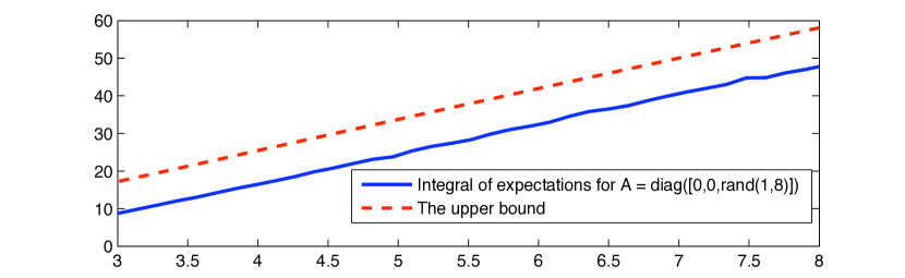
Figure 3. A numerical example suggesting that Proposition 3.1 is optimal: the left hand side is computed numerically for A = diag([0,0,rand(1,8)]) (a $10\times 10$ diagonal matrix of rank $8$) where rand command produces uniform distribution on $[0,1]$. It is plotted as a function of $\log(1/\delta)$. The upper bound in Proposition 3.1 (with $C=1$) is also plotted for comparison.

Proposition 3.1.

Let $A$ be a constant $d\times d$ matrix, and let $Q$ be a $d\times d$ random matrix, with the entries $q_{ij}$ independent complex $N(0,1)$ random variables. Then there exists a constant $C$ independent of $d$ and $A$, such that

$$\int_{0}^{1}\left|{\mathbb{E}}(\operatorname{tr}(tA+\delta Q)^{-1}A)\right|dt\leq C\operatorname{tr}\left(\frac{|A|}{\delta+|A|}\log\left(2+\frac{|A|}{\delta}\right)\right)\,,$$

where $|A|=\sqrt{AA^{*}}$.

In the proof we will need the following

Lemma 3.2.

The function $g(s)\stackrel{{\scriptstyle\rm{def}}}{{=}}\int_{{\mathbb{C}}}(1/|s+q|)e^{-|q|^{2}}d{\mathcal{L}}(q)$ is smooth for $s\in\mathbb{C}$, and

$$g(s)=\frac{\pi}{|s|}+{\mathcal{O}}\left(\frac{1}{|s|^{2}}\right)\,,\text{as }|s|\rightarrow\infty.$$

Proof.

The asymptotic expansion follows from the integrability of $|q|$, a change of variables, $q\mapsto 1+q/s$, and the method of stationary phase. ∎

Proof of Proposition 3.1.

Using the singular value decomposition for $A$, we may write $A=USV^{*}$, with $U$, $V$ unitary and $S$ a diagonal matrix with non-negative entries $\sigma_{1},...,\;\sigma_{d}$ on the diagonal. We note that

$$\operatorname{tr}((tA+\delta Q)^{-1}A)=\operatorname{tr}((tUSV^{*}+\delta Q)^{-1}USV^{*})=\operatorname{tr}((tS+\delta U^{*}QV)^{-1}S).$$

Since $U^{*}QV$ is a random matrix with the same probability distribution function as $Q$, we have

$${\mathbb{E}}(\operatorname{tr}((tA+\delta Q)^{-1}A))={\mathbb{E}}(\operatorname{tr}((tS+\delta Q)^{-1}S)).$$

Thus we may assume that $A$ is diagonal, with non-negative entries $\sigma_{1},\;...,\;\sigma_{d}$. We have

$$\operatorname{tr}((tA+\delta Q)^{-1}A)=\sum_{1}^{d}\frac{M_{ii}\sigma_{i}}{\det(tA+\delta Q)}$$

where here and below $M_{ij}$ is the $(i,j)$ minor of the matrix $tA+\delta Q$.

To compute ${\mathbb{E}}({M_{ii}\sigma_{i}}/{\det(tA+\delta Q)})$, we write

$$\det(tA+\delta Q)=(t\sigma_{i}+\delta q_{ii})M_{ii}+\sum_{j\not=i}(-1)^{j+i}\delta q_{ij}M_{ij}$$

and define

(3.3) $$\Sigma_{ii}\stackrel{{\scriptstyle\rm{def}}}{{=}}\left\{q\in{\mathbb{C}}^{d^{2}}\;:\;|(t\sigma_{i}+\delta q_{ii})M_{ii}|>\left|\sum_{j\not=i}(-1)^{j+i}\delta q_{ij}M_{ij}\right|\right\}\,.$$

Let ${\mathchoice{1\mskip-4.0mu{\rm{l}}}{1\mskip-4.0mu{\rm{l}}}{1\mskip-4.5mu{\rm{l}}}{1\mskip-5.0mu{\rm{l}}}}_{F}$ be the characteristic function of a set $F$. Then

(3.4) $${\mathbb{E}}\left(\frac{M_{ii}\sigma_{i}}{\det(tA+\delta Q)}\right)={\mathbb{E}}\left(\frac{M_{ii}\sigma_{i}}{\det(tA+\delta Q)}{\mathchoice{1\mskip-4.0mu{\rm{l}}}{1\mskip-4.0mu{\rm{l}}}{1\mskip-4.5mu{\rm{l}}}{1\mskip-5.0mu{\rm{l}}}}_{\Sigma_{ii}}\right)+{\mathbb{E}}\left(\frac{M_{ii}\sigma_{i}}{\det(tA+\delta Q)}{\mathchoice{1\mskip-4.0mu{\rm{l}}}{1\mskip-4.0mu{\rm{l}}}{1\mskip-4.5mu{\rm{l}}}{1\mskip-5.0mu{\rm{l}}}}_{\overline{\Sigma}_{ii}^{c}}\right)$$

since the boundary of $\Sigma_{ii}$ has measure $0$.

Now,

$$\begin{split}{\mathbb{E}}\left(\frac{M_{ii}\sigma_{i}}{\det(tA+\delta Q)}{\mathchoice{1\mskip-4.0mu{\rm{l}}}{1\mskip-4.0mu{\rm{l}}}{1\mskip-4.5mu{\rm{l}}}{1\mskip-5.0mu{\rm{l}}}}_{\Sigma_{ii}}\right)&={\mathbb{E}}\left(\frac{M_{ii}\sigma_{i}}{(t\sigma_{i}+\delta q_{ii})M_{ii}}\left(1+\frac{\sum_{j\not=i}^{d}(-1)^{j+i}\delta q_{ij}M_{ij}}{(t\sigma_{i}+\delta q_{ii})M_{ii}}\right)^{-1}{\mathchoice{1\mskip-4.0mu{\rm{l}}}{1\mskip-4.0mu{\rm{l}}}{1\mskip-4.5mu{\rm{l}}}{1\mskip-5.0mu{\rm{l}}}}_{\Sigma_{ii}}\right)\\ &={\mathbb{E}}\left(\frac{\sigma_{i}}{(t\sigma_{i}+\delta q_{ii})}\sum_{k=0}^{\infty}\left(-\frac{\sum_{j\not=i}^{d}(-1)^{j+i}\delta q_{ij}M_{ij}}{(t\sigma_{i}+\delta q_{ii})M_{ii}}\right)^{k}{\mathchoice{1\mskip-4.0mu{\rm{l}}}{1\mskip-4.0mu{\rm{l}}}{1\mskip-4.5mu{\rm{l}}}{1\mskip-5.0mu{\rm{l}}}}_{\Sigma_{ii}}\right).\end{split}$$

We recall that the set $\Sigma_{ii}$ is chosen so that the infinite sum converges.

The set $\Sigma_{ii}$ is invariant under the mapping

(3.5) $$q_{i1},...,q_{i,i-1},q_{i,i+1},...,q_{i,d}\mapsto e^{i\varphi}q_{i1},...,e^{i\varphi}q_{i,i-1},e^{i\varphi}q_{i,i+1},...,e^{i\varphi}q_{i,d}$$

for any real number $\varphi$. Since $M_{ij}$’s are independent of $q_{ij}$, $\sum_{j\not=i}^{d}(-1)^{j+i}\delta q_{ij}M_{ij}$ is homogeneous of degree $1$ under this same mapping and $(t\sigma_{i}+\delta q_{ii})M_{ii}$ is independent of $q_{ij}$ for $j\not=i$, we find that

$${\mathbb{E}}\left(\frac{M_{ii}\sigma_{i}}{\det(tA+\delta Q)}{\mathchoice{1\mskip-4.0mu{\rm{l}}}{1\mskip-4.0mu{\rm{l}}}{1\mskip-4.5mu{\rm{l}}}{1\mskip-5.0mu{\rm{l}}}}_{\Sigma_{ii}}\right)={\mathbb{E}}\left(\frac{\sigma_{i}}{(t\sigma_{i}+\delta q_{ii})}{\mathchoice{1\mskip-4.0mu{\rm{l}}}{1\mskip-4.0mu{\rm{l}}}{1\mskip-4.5mu{\rm{l}}}{1\mskip-5.0mu{\rm{l}}}}_{\Sigma_{ii}}\right).$$

We do a similar computation for the second term of (3.4):

$${\mathbb{E}}\left(\frac{M_{ii}\sigma_{i}}{\det(tA+\delta Q)}{\mathchoice{1\mskip-4.0mu{\rm{l}}}{1\mskip-4.0mu{\rm{l}}}{1\mskip-4.5mu{\rm{l}}}{1\mskip-5.0mu{\rm{l}}}}_{\overline{\Sigma}_{ii}^{c}}\right)={\mathbb{E}}\left(\frac{M_{ii}\sigma_{i}}{\sum_{j\not=i}^{d}(-1)^{j+i}\delta q_{ij}M_{ij}}\left(1+\frac{(t\sigma_{i}+\delta q_{ii})}{\sum_{j\not=i}^{d}(-1)^{j+i}\delta q_{ij}M_{ij}}\right)^{-1}{\mathchoice{1\mskip-4.0mu{\rm{l}}}{1\mskip-4.0mu{\rm{l}}}{1\mskip-4.5mu{\rm{l}}}{1\mskip-5.0mu{\rm{l}}}}_{\overline{\Sigma}_{ii}^{c}}\right)$$

$$={\mathbb{E}}\left(\frac{M_{ii}\sigma_{i}}{\sum_{j\not=i}^{d}(-1)^{j+i}\delta q_{ij}M_{ij}}\sum_{k=0}^{\infty}\left(-\frac{(t\sigma_{i}+\delta q_{ii})}{\sum_{j\not=i}^{d}(-1)^{j+i}\delta q_{ij}M_{ij}}\right)^{k}{\mathchoice{1\mskip-4.0mu{\rm{l}}}{1\mskip-4.0mu{\rm{l}}}{1\mskip-4.5mu{\rm{l}}}{1\mskip-5.0mu{\rm{l}}}}_{\overline{\Sigma}_{ii}^{c}}\right)=0\,,$$

using, as before, the invariance properties of $\Sigma_{ii}$ and the homogeneity of

$${\sum_{j\not=i}^{d}(-1)^{j+i}\delta q_{ij}M_{ij}}\,.$$

Thus we have

(3.6) $${\mathbb{E}}(\operatorname{tr}(tA+\delta Q)^{-1}A)=\sum_{i=1}^{d}{\mathbb{E}}\left(\frac{\sigma_{i}}{(t\sigma_{i}+\delta q_{ii})}{\mathchoice{1\mskip-4.0mu{\rm{l}}}{1\mskip-4.0mu{\rm{l}}}{1\mskip-4.5mu{\rm{l}}}{1\mskip-5.0mu{\rm{l}}}}_{\Sigma_{ii}}\right).$$

Now,

$$\begin{split}\left|\int_{0}^{1}{\mathbb{E}}\left(\frac{\sigma_{i}}{(t\sigma_{i}+\delta q_{ii})}{\mathchoice{1\mskip-4.0mu{\rm{l}}}{1\mskip-4.0mu{\rm{l}}}{1\mskip-4.5mu{\rm{l}}}{1\mskip-5.0mu{\rm{l}}}}_{\Sigma_{ii}}\right)dt\right|&\leq\int_{0}^{1}{\mathbb{E}}\left(\frac{\sigma_{i}}{|t\sigma_{i}+\delta q_{ii}|}\right)dt=\int_{0}^{1}{\mathbb{E}}\left(\frac{\sigma_{i}/\delta}{|t\sigma_{i}/\delta+q_{ii}|}\right)dt\\ &=\int_{0}^{\sigma_{i}/\delta}{\mathbb{E}}\left(\frac{1}{|s+q_{ii}|}\right)ds=\frac{1}{\pi}\int_{0}^{\sigma_{i}/\delta}g(s)ds\end{split}$$

where $g$ is the function defined in Lemma 3.2. Using this, (3.6), and the results of Lemma 3.2 proves the proposition. ∎

Lemma 3.3.

Let $F,\;G$ be $d\times d$ matrices, with $F$ invertible, and let $\beta=\|F^{-1}\|.$ Then

$${\mathbb{E}}\Big{(}\operatorname{tr}\big{(}(F+\delta Q)^{-1}G\big{)}\Big{)}=\operatorname{tr}\Big{(}F^{-1}G\Big{)}\big{(}1+O(e^{-1/4(\delta\beta d)^{2}})\big{)}+{\mathcal{O}}\left(\frac{1}{\delta}\|G\|d^{4}e^{-1/4(d\beta\delta)^{2}}\right).$$

The implicit constant in the error term is independent of $F$ and $G$.

Proof.

We first note that if we replace $F$ by its singular value decomposition, $F=USV^{*}$, then

$${\mathbb{E}}\Big{(}\operatorname{tr}\big{(}(F+\delta Q)^{-1}G\big{)}\Big{)}={\mathbb{E}}\Big{(}\operatorname{tr}\big{(}(S+\delta Q)^{-1}(U^{*}GV)\big{)}\Big{)}$$

and

$$\operatorname{tr}\big{(}F^{-1}G\big{)}=\operatorname{tr}\big{(}S^{-1}U^{*}GV\big{)}.$$

Thus we may assume that $F$ is a diagonal matrix.

Our proof then resembles the proof of Proposition 3.1. Let $\chi\in L^{\infty}({\mathbb{R}}_{+})$ be the characteristic function of $(-\infty,1/2]$, and, if $A=(a_{ij})$, let $\|A\|_{\sup}=\sup_{ij}|a_{ij}|.$ We write

(3.7) $${\mathbb{E}}\Big{(}\operatorname{tr}\big{(}(F+\delta Q)^{-1}G\big{)}\Big{)}={\mathbb{E}}\Big{(}\operatorname{tr}\big{(}(F+\delta Q)^{-1}G\big{)}\chi(d\|Q\|_{\sup}\delta\beta)\Big{)}\\ +{\mathbb{E}}\Big{(}\operatorname{tr}\big{(}(F+\delta Q)^{-1}G\big{)}(1-\chi(d\|Q\|_{\sup}\delta\beta))\Big{)}.$$

For the first term,

$${\mathbb{E}}\Big{(}\operatorname{tr}\big{(}(F+\delta Q)^{-1}G\big{)}\chi(d\|Q\|_{\sup}\delta\beta)\Big{)}={\mathbb{E}}\Big{(}\operatorname{tr}\Big{(}F^{-1}\sum_{0}^{\infty}(-\delta(QF^{-1})^{j}G\Big{)}\chi(d\|Q\|_{\sup}\delta\beta))\Big{)}.$$

Using the fact that the cut-off $\chi(d\|Q\|_{\sup}\delta\beta)$ is invariant under rotations of the $q_{ij}$ and that the $q_{ij}$ are complex and independent, we find

$${\mathbb{E}}\Big{(}\operatorname{tr}\big{(}(F+\delta Q)^{-1}G\big{)}\chi(d\|Q\|_{\sup}\delta\beta)\Big{)} =\operatorname{tr}\big{(}F^{-1}G)\mu(Q:\|Q\|_{\sup}<1/2\delta\beta d)$$

(3.8) $$=\operatorname{tr}\big{(}F^{-1}G)(1+{\mathcal{O}}(d^{2}e^{-1/4(\delta\beta d)^{2}}))\,.$$

Now we consider the remaining term of (3.7). In a way similar to the proof of Proposition 3.1, we denote the diagonal entries of $F$ by $f_{ii}=\sigma_{i}$, and by $M_{ij}$ the $(i,j)$ minor of $F+\delta Q$. If $G=(g_{ij})$, we have

$${\mathbb{E}}\Big{(}\operatorname{tr}\big{(}(F+\delta Q)^{-1}G\big{)}(1-\chi(d\|Q\|_{\sup}\delta\beta))\Big{)}={\mathbb{E}}\Big{(}\sum_{i,j}\frac{(-1)^{i+j}M_{ji}g_{ji}}{\det(F+\delta Q)}(1-\chi(d\|Q\|_{\sup}\delta\beta))\Big{)}.$$

Just as in the proof of Proposition 3.1, to compute

$${\mathbb{E}}\Big{(}\frac{M_{ii}g_{ii}}{\det(F+\delta Q)}(1-\chi(d\|Q\|_{\sup}\delta\beta))\Big{)}$$

we write

$$\det(F+\delta Q)=(\sigma_{i}+\delta q_{ii})M_{ii}+\sum_{j\not=i}(-1)^{j+i}\delta q_{ij}M_{ij}$$

and define $\Sigma_{ii}$ as in (3.3). Proceeding almost exactly as in the proof of Proposition 3.1, using that both $\Sigma_{ii}$ and the support of $(1-\chi(d\|Q\|_{\sup}\delta\beta))$ are invariant under the mapping (3.5), we get that

$${\mathbb{E}}\Big{(}\frac{M_{ii}g_{ii}}{\det(F+\delta Q)}(1-\chi(d\|Q\|_{\sup}\delta\beta))\Big{)}={\mathbb{E}}\left(\frac{g_{ii}}{(\sigma_{i}+\delta q_{ii})}{\mathchoice{1\mskip-4.0mu{\rm{l}}}{1\mskip-4.0mu{\rm{l}}}{1\mskip-4.5mu{\rm{l}}}{1\mskip-5.0mu{\rm{l}}}}_{\Sigma_{ii}}(1-\chi(d\|Q\|_{\sup}\delta\beta))\right).$$

But

$$\left|{\mathbb{E}}\left(\frac{g_{ii}}{(\sigma_{i}+\delta q_{ii})}{\mathchoice{1\mskip-4.0mu{\rm{l}}}{1\mskip-4.0mu{\rm{l}}}{1\mskip-4.5mu{\rm{l}}}{1\mskip-5.0mu{\rm{l}}}}_{\Sigma_{ii}}(1-\chi(d\|Q\|_{\sup}\delta\beta))\right)\right|\leq C\frac{\|G\|}{\delta}d^{2}e^{-1/4(d\delta\beta)^{2}}.$$

To compute

$${\mathbb{E}}\Big{(}\frac{(-1)^{i+j}M_{ji}g_{ji}}{\det(F+\delta Q)}(1-\chi(d\|Q\|_{\sup}\delta\beta))\Big{)}$$

when $i\not=j$, we write

(3.9) $$\det(F+\delta Q)=\delta q_{ji}M_{ji}(-1)^{i+j}+(\sigma_{i}+\delta q_{ii})M_{ii}+\sum_{k\not=i,j}(-1)^{k+i}\delta q_{ki}M_{ki}$$

and define

$$\Sigma_{ji}\stackrel{{\scriptstyle\rm{def}}}{{=}}\left\{q\in{\mathbb{C}}^{d^{2}}\;:\;|\delta q_{ji}M_{ji}|>\left|(\sigma_{i}+\delta q_{ii})M_{ii}+\sum_{i\neq k\neq j}(-1)^{k+i}\delta q_{ki}M_{ki}\right|\right\}\,.$$

Following the proof of Proposition 3.1 but treating the term $\delta q_{ji}M_{ji}$ as the distinguished one in the expansion of the determinant (3.9) and using the invariance of $\Sigma_{ji}$ under rotations of $q_{ji}$, we find that

$${\mathbb{E}}\left(\frac{(-1)^{i+j}M_{ji}g_{ji}}{\det(F+\delta Q)}(1-\chi(d\|Q\|_{\sup}\delta\beta))\right)\\ ={\mathbb{E}}\left(\frac{(-1)^{i+j}M_{ji}g_{ji}}{(\sigma_{i}+\delta q_{ii})M_{ii}+\sum_{k\not=i,j}(-1)^{k+i}\delta q_{ki}M_{ki}}{\mathchoice{1\mskip-4.0mu{\rm{l}}}{1\mskip-4.0mu{\rm{l}}}{1\mskip-4.5mu{\rm{l}}}{1\mskip-5.0mu{\rm{l}}}}_{\overline{\Sigma}_{ji}^{c}}(1-\chi(d\|Q\|_{\sup}\delta\beta))\right).$$

Since on the support of ${\mathchoice{1\mskip-4.0mu{\rm{l}}}{1\mskip-4.0mu{\rm{l}}}{1\mskip-4.5mu{\rm{l}}}{1\mskip-5.0mu{\rm{l}}}}_{\overline{\Sigma}_{ji}^{c}}$

$$|M_{ji}|\leq\frac{1}{\delta|q_{ji}|}\left|(\sigma_{i}+\delta q_{ii})M_{ii}+\sum_{k\not=i,j}(-1)^{k+i}\delta q_{ki}M_{ki})\right|$$

we find

$$\left|{\mathbb{E}}\left(\frac{(-1)^{i+j}M_{ji}g_{ji}}{\det(F+\delta Q)}(1-\chi(d\|Q\|_{\sup}\delta\beta))\right)\right|\leq C\frac{\|G\|}{\delta}d^{2}e^{-1/4(d\delta\beta)^{2}}.$$

∎

Our proof of Proposition 4.1 in the next section will use Proposition 3.5. To prove this proposition we will need several preliminary results.

The first lemma below follows from well-known facts about eigenvalues of complex Gaussian ensemble. We give a direct proof suggested to us by Mark Rudelson:

Lemma 3.4.

Let $A=(a_{1},...,a_{d})$, with $a_{i}\in\mathbb{C}^{d}$. Then, with the notation of (3.1),

$$\int_{\|A\|_{HS}\leq 1}|\det A|^{-1}d{\mathcal{L}}(A)<\infty\,.$$

Proof.

We begin by introducing some more notation. For $p\leq d$, $p\in{\mathbb{N}}$, $v\in\mathbb{C}^{d}$ denote by ${\mathcal{P}}_{p}v$ projection onto the subspace spanned (over the complex numbers) by $a_{1},...,a_{p}$. This of course depends on $a_{1},...,a_{p}$, but we omit this in our notation for simplicity.

Using the Graham-Schmidt process, we can, if $A$ is invertible (as it is off a set of measure $0$), write the matrix $A=UR$, with $U$ a unitary matrix and $R$ being upper triangular. The diagonal entries of $R$ are then given by $\|a_{1}\|$ and $\|(1-{\mathcal{P}}_{p-1})a_{p}\|$, $p=2,...,d$. Thus

$$|\det A|=\|a_{1}\|\|(1-{\mathcal{P}}_{1})a_{2}\|\|(1-{\mathcal{P}}_{2})a_{3}\|\cdot\cdot\cdot\|(1-{\mathcal{P}}_{d-1})a_{d}\|.$$

Note that

$$\|a_{1}\|\|(1-{\mathcal{P}}_{1})a_{2}\|\|(1-{\mathcal{P}}_{2})a_{3}\|\cdot\cdot\cdot\|(1-{\mathcal{P}}_{d-2})a_{d-1}\|$$

is independent of $a_{d}$, that is, independent of $a_{1d},a_{2d},...,a_{dd}$. Therefore

$$\int_{\|A\|_{HS}\leq 1}|\det A|^{-1}d{\mathcal{L}}(A)$$

$$=\int_{\|A\|_{HS}\leq 1}\frac{1}{\|a_{1}\|\|(1-{\mathcal{P}}_{1})a_{2}\|\cdot\cdot\cdot\|(1-{\mathcal{P}}_{d-2})a_{d-1}\|}\frac{d{\mathcal{L}}(a_{d})d{\mathcal{L}}(a_{d-1})...d{\mathcal{L}}(a_{1})}{\|(1-{\mathcal{P}}_{d-1})a_{d}\|}$$

$$\leq\int_{\|a_{1}\|\leq 1}\cdot\cdot\cdot\int_{\|a_{d}\|\leq 1}\frac{d{\mathcal{L}}(a_{d})}{\|(1-{\mathcal{P}}_{d-1})a_{d}\|}\frac{d{\mathcal{L}}(a_{d-1})...d{\mathcal{L}}(a_{1})}{\|a_{1}\|\|(1-{\mathcal{P}}_{1})a_{2}\|\cdot\cdot\cdot\|(1-{\mathcal{P}}_{d-2})a_{d-1}\|}.$$

The value of $\int_{\|a_{d}\|\leq 1}1/{\|(1-{\mathcal{P}}_{d-1})a_{d}\|}d{\mathcal{L}}(a_{d})$ depends only on $d$ and the rank of the space spanned by $a_{1},...,a_{d-1}$. We find $1/\|(1-{\mathcal{P}}_{d-1})a_{d}\|$ is locally integrable over ${\mathbb{R}}^{2d}\simeq\mathbb{C}^{d}$, because $a_{d}\in\mathbb{C}^{d}$ and the space spanned by $a_{1},...,a_{d-1}$ has complex dimension at most $d-1$.Therefore

(3.10) $$\int_{\|a_{d}\|\leq 1}\frac{1}{\|(1-{\mathcal{P}}_{d-1})a_{d}\|}d{\mathcal{L}}(a_{d})\leq C<\infty.$$

Here the constant $C$ can be chosen independent of $a_{1},...,a_{d-1}$, as the maximum of the integral in (3.10) occurs when $a_{1},...,a_{d-1}$ span a $d-1$ dimensional vector space. The proof follows by iterating the above argument. ∎

Proposition 3.5.

Let $A(s,t)$ be a $d\times d$ matrix depending smoothly on $(s,t)\in U\subset\mathbb{C}^{2}$. Let $Q$ denote a $d\times d$ random matrix, with each entry an independent complex $N(0,1)$ random variable. Then for $\delta>0,$ $(s,t)\in U$, ${\mathbb{E}}(\operatorname{tr}((A(s,t)+\delta Q)^{-1}\partial_{t}A)$ is smooth on $U$, and

$$\partial_{s}{\mathbb{E}}\big{(}\operatorname{tr}((A(s,t)+\delta Q)^{-1}\partial_{t}A)\big{)}=\partial_{t}{\mathbb{E}}\big{(}\operatorname{tr}((A(s,t)+\delta Q)^{-1}\partial_{s}A)\big{)}.$$

This proposition has the following corollary.

Corollary 3.6.

Let $M$, $B$, be $d\times d$ matrices independent of $s$ and $t$. Then

$$\int_{0}^{1}{\mathbb{E}}\Big{(}\operatorname{tr}\big{(}(s{B}+{M}+\delta{Q})^{-1}{B}\big{)}\Big{)}ds=\int_{0}^{1}{\mathbb{E}}\Big{(}\operatorname{tr}\big{(}({B}+t{M}+\delta{Q})^{-1}{M}\big{)}\Big{)}dt$$

$$\ \ \ -\,\int_{0}^{1}{\mathbb{E}}\Big{(}\operatorname{tr}\big{(}(t{M}+\delta{Q})^{-1}{M}\big{)}\Big{)}dt\hskip 11.38109pt+\int_{0}^{1}{\mathbb{E}}\Big{(}\operatorname{tr}\big{(}(s{B}+\delta{Q})^{-1}{B}\big{)}\Big{)}ds.$$

Proof.

Using the previous proposition, this follows from the Fundamental Theorem of Calculus:

$$\int_{0}^{1}{\mathbb{E}}\Big{(}\operatorname{tr}\big{(}(s{B}+{M}+\delta{Q})^{-1}{B}\big{)}\Big{)}ds-\int_{0}^{1}{\mathbb{E}}\Big{(}\operatorname{tr}\big{(}(s{B}+\delta{Q})^{-1}{B}\big{)}\Big{)}ds$$

$$=\int_{0}^{1}\partial_{t}\int_{0}^{1}{\mathbb{E}}\operatorname{tr}\left((s{B}+t{M}+\delta{Q})^{-1}B\right)dsdt$$

$$=\int_{0}^{1}\partial_{s}\int_{0}^{1}{\mathbb{E}}\operatorname{tr}\left((s{B}+t{M}+\delta{Q})^{-1}M\right)dtds$$

$$=\int_{0}^{1}{\mathbb{E}}\Big{(}\operatorname{tr}\big{(}({B}+t{M}+\delta{Q})^{-1}{M}\big{)}\Big{)}dt-\int_{0}^{1}{\mathbb{E}}\Big{(}\operatorname{tr}\big{(}(t{M}+\delta{Q})^{-1}{M}\big{)}\Big{)}dt.$$

∎

Proposition 3.5 follows from the subsequent two lemmas.

Lemma 3.7.

Let $A(s,t)$, $B(s,t)$ be $d\times d$ matrices depending smoothly on $(s,t)\in U\subset\mathbb{C}^{2}$. With $Q$ a random matrix as in Proposition 3.5 and $\delta>0$,

$${\mathbb{E}}\left(\operatorname{tr}\big{(}(A(s,t)+\delta Q)^{-1}B(s,t)\big{)}\right)\in C^{\infty}(U).$$

Proof.

We prove the lemma by writing the expected value as an integral:

$${\mathbb{E}}\left(\operatorname{tr}((A+\delta Q)^{-1}B)\right) =\int\operatorname{tr}((A+\delta Q)^{-1}B)e^{-\|Q\|^{2}_{HS}}d{\mathcal{L}}(Q)$$

$$=\int\operatorname{tr}((\delta Q)^{-1}B)e^{-\|Q-\frac{1}{\delta}A\|^{2}_{HS}}d{\mathcal{L}}(Q).$$

Now, for a $d\times d$ matrix $\tilde{B}$, $|\operatorname{tr}((\delta Q)^{-1}\tilde{B})|\leq{C}|\det Q|^{-1}\|\tilde{B}\|\|Q\|^{d-1}/{\delta}$, where the constant $C$ depends on $d$. Moreover,

$$|\partial_{s}^{j}\partial_{t}^{k}e^{-\|Q-\frac{1}{\delta}A\|^{2}_{HS}}|\leq C_{j,k,d}(\sum_{j^{\prime}\leq j,k^{\prime}\leq k}\|\partial_{s}^{j^{\prime}}\partial_{t}^{k^{\prime}}A\|)\left(\frac{\|Q\|}{\delta^{2}}\right)^{j+k}e^{-\|Q-\frac{1}{\delta}A\|^{2}_{HS}}.$$

Since, using Lemma 3.4 $\int|\det Q|^{-1}(1+\|Q\|)^{m}e^{-\|Q-\frac{1}{\delta}A\|^{2}_{HS}}d{\mathcal{L}}(Q)<\infty$, for any finite $m$, the smoothness of $A$ and $B$ proves the lemma. ∎

If $M$ is an invertible matrix depending smoothly on $s$ and $t$, then

(3.11) $$\operatorname{tr}(M^{-1}\partial_{t}M)=\frac{\partial_{t}\det M}{\det M}\;\text{and}\;\partial_{s}\operatorname{tr}(M^{-1}M_{t})=\partial_{t}\operatorname{tr}(M^{-1}M_{s}).$$

The lemma below shows that something similar is true when taking expected values, even though the matrices under consideration are not invertible for some values of the random variable.

Lemma 3.8.

Let $A(s,t)$ be a $d\times d$ matrix depending smoothly on $(s,t)\in U\subset\mathbb{C}^{2}$, and $Q$ a random matrix as in Proposition 3.5. Then for $\delta>0$

$$\partial_{s}{\mathbb{E}}\left(\operatorname{tr}((A+\delta Q)^{-1}\partial_{t}A)\right)=\partial_{t}{\mathbb{E}}\left(\operatorname{tr}((A+\delta Q)^{-1}\partial_{s}A)\right).$$

Proof.

Let $\chi_{\epsilon}\in C^{\infty}({\mathbb{R}})$ satisfy $\chi_{\epsilon}(x)=1$ for $|x|<\epsilon/2$ and $\chi_{\epsilon}(x)=0$ for $|x|>\epsilon$. Then

$$\partial_{s}{\mathbb{E}}\left(\operatorname{tr}((A+\delta Q)^{-1}\partial_{t}A)\right) =\partial_{s}{\mathbb{E}}\left(\chi_{\epsilon}(\det(A+\delta Q))\operatorname{tr}((A+\delta Q)^{-1}\partial_{t}A)\right)$$

(3.12) $$+\partial_{s}{\mathbb{E}}\left(\big{(}1-\chi_{\epsilon}(\det(A+\delta Q))\big{)}\operatorname{tr}\big{(}(A+\delta Q)^{-1}\partial_{t}A\big{)}\right).$$

Now

$$\partial_{s}{\mathbb{E}}\left(\big{(}1-\chi_{\epsilon}(\det(A+\delta Q))\big{)}\operatorname{tr}\big{(}(A+\delta Q)^{-1}\partial_{t}A\big{)}\right)$$

$$=\int\big{(}1-\chi_{\epsilon}(\det(A+\delta Q))\big{)}\partial_{s}\operatorname{tr}\big{(}(A+\delta Q)^{-1}\partial_{t}A\big{)}e^{-\|Q\|^{2}_{HS}}d{\mathcal{L}}(Q)$$

$$-\int\chi_{\epsilon}^{\prime}(\det(A+\delta Q))\big{(}\partial_{s}\det(A+\delta Q)\big{)}\operatorname{tr}\big{(}(A+\delta Q)^{-1}\partial_{t}A\big{)}e^{-\|Q\|^{2}_{HS}}d{\mathcal{L}}(Q)$$

where we can freely interchange differentiation and integration since the integrand is smooth and it and its derivatives are integrable. But using (3.11), we get

$$\partial_{s}{\mathbb{E}}\left(\big{(}1-\chi_{\epsilon}(\det(A+\delta Q))\big{)}\operatorname{tr}\big{(}(A+\delta Q)^{-1}\partial_{t}A\big{)}\right)$$

$$=\int\big{(}1-\chi_{\epsilon}(\det(A+\delta Q))\big{)}\partial_{t}\operatorname{tr}\big{(}(A+\delta Q)^{-1}\partial_{s}A\big{)}e^{-\|Q\|^{2}_{HS}}d{\mathcal{L}}(Q)$$

$$-\int\chi_{\epsilon}^{\prime}(\det(A+\delta Q))\partial_{t}\det(A+\delta Q)\operatorname{tr}\big{(}(A+\delta Q)^{-1}\partial_{s}A\big{)}e^{-\|Q\|^{2}_{HS}}d{\mathcal{L}}(Q)$$

$$=\partial_{t}{\mathbb{E}}\left(\big{(}1-\chi_{\epsilon}(\det(A+\delta Q))\big{)}\operatorname{tr}\big{(}(A+\delta Q)^{-1}\partial_{s}A\big{)}\right).$$

On the other hand, the first term on the right in (3) satisfies

$$\lim_{\epsilon\downarrow 0}\partial_{s}{\mathbb{E}}\left(\chi_{\epsilon}(\det(A+\delta Q))(\operatorname{tr}((A+\delta Q)^{-1}\partial_{t}A)\right)$$

$$=\lim_{\epsilon\downarrow 0}\partial_{s}\int\chi_{\epsilon}(\det(A+\delta Q))(\operatorname{tr}((A+\delta Q)^{-1}\partial_{t}A)e^{-\|Q\|^{2}_{HS}}d{\mathcal{L}}(Q)$$

$$=\lim_{\epsilon\downarrow 0}\partial_{s}\int\chi_{\epsilon}(\det(\delta Q))(\operatorname{tr}((\delta Q)^{-1}\partial_{t}A)e^{-\|Q-\frac{1}{\delta}A\|^{2}_{HS}}d{\mathcal{L}}(Q)=0$$

since $(\operatorname{tr}((\delta Q)^{-1}\partial_{t}A)e^{-\|Q-\frac{1}{\delta}A\|^{2}_{HS}}$ and its $s$ derivative are both in $L^{1}$, using Lemma 3.4. ∎

4. Reduction to a deterministic problem

In this section we will show how to reduce the random problem problem to a deterministic one. That will be done using the singular value decomposition of the matrix $f_{N}$.

Let $A$ be a square matrix, and let $USV^{*}$ be a singular value decomposition for $A$. We make the following simple observation: for $\psi\in{\mathcal{C}}^{\infty}_{\rm{c}}({\mathbb{R}},{\mathbb{R}})$ equal to $1$ on $[-1,1]$,

(4.1) $$(A+\alpha\psi(AA^{*}/\alpha^{2})UV^{*})^{-1}={{\mathcal{O}}}(1/\alpha)\;:\;\ell^{2}\longrightarrow\ell^{2}\,,$$

which becomes totally transparent by writing $\psi(AA^{*}/\alpha^{2})UV^{*}=U\psi((S/\alpha)^{2})V^{*}$.

The random problem is reduced to a deterministic one by using an operator of the form (4.1).

Proposition 4.1.

For a smooth curve $\gamma$ define

(4.2) $$I_{N}(\gamma)\stackrel{{\scriptstyle\rm{def}}}{{=}}\int_{\gamma}\mathbb{E}\operatorname{tr}(f_{N}+\delta Q_{N}-z)^{-1}dz\,$$

where $Q_{N}$ is a complex $N^{n}\times N^{n}$ matrix, with entries indepent $N(0,1)$ random variables. Let $f_{N}=U_{N}S_{N}V_{N}^{*}$ be a singular value decomposition of $f_{N}$, and let $\psi\in{\mathcal{C}}^{\infty}_{\rm{c}}({\mathbb{R}};[0,1])$ be equal to $1$ on $[-1,1]$. If

(4.3) $$0\in\gamma\,,\ \ |\gamma|<\alpha/4\,,\ \ \ \ \delta\ll\alpha\,,$$

then

(4.4) $$\begin{split}&\int_{\gamma}\mathbb{E}\operatorname{tr}(f_{N}+\delta Q_{N}(\omega)-z)^{-1}dz=\,\\ &\ \ \ \ \int_{\gamma}\mathbb{E}\operatorname{tr}({f_{N}+\alpha\psi(f_{N}f_{N}^{*}/\alpha^{2})U_{N}V_{N}^{*}}+\delta Q_{N}(\omega)-z)^{-1}dz+E_{1}=\,\\ &\ \ \ \ \int_{\gamma}\operatorname{tr}({f_{N}+\alpha\psi(f_{N}f_{N}^{*}/\alpha^{2})U_{N}V_{N}^{*}}-z)^{-1}dz+E_{2}\,,\end{split}$$

where

(4.5) $$E_{1},E_{2}={\mathcal{O}}\left(d\log\left(\frac{\alpha}{\delta}\right)+\frac{N^{4n}}{\delta}e^{-\alpha^{2}/4(3N^{n}\delta)^{2}}\right)\,,$$

and $d=\operatorname{rank}{\mathchoice{1\mskip-4.0mu{\rm{l}}}{1\mskip-4.0mu{\rm{l}}}{1\mskip-4.5mu{\rm{l}}}{1\mskip-5.0mu{\rm{l}}}}_{\operatorname{supp}\psi}\left({f_{N}f_{N}^{*}}/{\alpha^{2}}\right)$.

The proof of this proposition will use the following lemma.

Lemma 4.2.

Let $f_{N},\;U_{N},\;S_{N},\;V_{N},\;\psi,\;\delta,\;d,$ and $\alpha$ be as in the statement of Proposition 4.1. Let $\chi\in L^{\infty}({\mathbb{R}})$ be the characteristic function for the support of $\psi$. Then, if $|z|\leq\alpha/4$,

$$\left|\int_{0}^{1}{\mathbb{E}}\operatorname{tr}\left((f_{N}+s\alpha\chi(f_{N}f_{N}^{*}/\alpha^{2})U_{N}V_{N}^{*}-z+\delta Q)^{-1}\alpha\chi(f_{N}f_{N}^{*}/\alpha^{2})U_{N}V_{N}^{*}\right)ds\right|$$

satisfies the bound (4.5).

Proof.

First suppose that for a $m\times m$ matrix $\tilde{A}$,

(4.6) $$\tilde{A}=\left(\begin{array}[]{cc}\tilde{A}_{11}&\tilde{A}_{12}\\ \tilde{A}_{21}&\tilde{A}_{22}\end{array}\right)\ \ \ \ \ \text{and}\ \ \ \ \ \tilde{A}^{-1}=\left(\begin{array}[]{cc}\tilde{B}_{11}&\tilde{B}_{12}\\ \tilde{B}_{21}&\tilde{B}_{22}\end{array}\right)$$

with $\tilde{A}_{11},$ $\tilde{B}_{11}$ $d\times d$ matrices and $\tilde{A}_{11},$ $\tilde{B}_{11}$ $(m-d)\times(m-d)$ matrices. Then if $\tilde{A}_{22}$ is invertible, we have the Schur complement formula,

(4.7) $$\tilde{B}_{11}=\left(\tilde{A}_{11}+\tilde{A}_{12}\tilde{A}_{22}^{-1}\tilde{A}_{21}\right)^{-1}\,,$$

see [18] for a review of some of its applications in spectral theory.

We note, using $\psi(AA^{*}/\alpha^{2})UV^{*}=U\psi((S/\alpha)^{2})V^{*}$ and the unitarity of $U_{N}$, $V_{N}$,

(4.8) $${\mathbb{E}}\operatorname{tr}\big{(}(f_{N}+s\alpha\chi(f_{N}f_{N}^{*}/\alpha^{2})U_{N}V_{N}^{*}-z+\delta Q_{N})^{-1}\alpha\chi(f_{N}f_{N}^{*}/\alpha^{2})U_{N}V_{N}^{*}\big{)}\\ ={\mathbb{E}}\operatorname{tr}\big{(}(S_{N}+s\alpha\chi(S_{N}S_{N}^{*}/\alpha^{2})-U_{N}^{*}zV_{N}+\delta Q_{N})^{-1}\alpha\chi(S_{N}S_{N}^{*}/\alpha^{2})\big{)}.$$

The main idea of the proof will be to effectively reduce the dimension of the matrices we work with, from $N^{n}$ to $d$. We can assume that $U_{N}$, $V_{N}$, $S_{N}$ are chosen so that the diagonal elements $\sigma_{1},...,\sigma_{N^{n}}$ of $S_{N}$ satisfy $\sigma_{1}\leq\sigma_{2}\cdot\cdot\cdot\leq\sigma_{N^{n}}$. Let ${\mathcal{J}}$ denote projection onto the range of $\chi(S_{N}^{2}/\alpha^{2})$, which is the same as projection off of the kernel of $\chi(S_{N}^{2}/\alpha^{2})$. Then

$${\mathcal{J}}=\left(\begin{array}[]{cc}I_{d}&0\\ 0&0\end{array}\right).$$

and $\alpha\chi(S_{N}^{2}/\alpha^{2})$ takes the form

$$\left(\begin{array}[]{cc}\alpha I_{d}&0\\ 0&0\end{array}\right).$$

We also write

$$S_{N}+s\alpha\chi(S_{N}S_{N}^{*}/\alpha^{2})-U_{N}^{*}zV_{N}=\left(\begin{array}[]{cc}s\alpha I_{d}+A_{11}&A_{12}\\ A_{21}&A_{22}\end{array}\right),$$

and

$$Q_{N}=\left(\begin{array}[]{cc}Q_{11}&Q_{12}\\ Q_{21}&Q_{22}\end{array}\right)$$

where $A_{11},\;Q_{11}$ are $d\times d$-dimensional matrices, and $A_{22},\;Q_{22}$ are $(N^{n}-d)\times(N^{n}-d)$-dimensional. Since $S_{N}$ is diagonal and $|z|\leq\alpha/4$, we have $\|A_{12}\|\leq\alpha/4$, $\|A_{21}\|\leq\alpha/4$.

Using this notation, we have that $A_{22}$ is invertible, with norm at most $4/3\alpha$. Now restrict $Q_{N}$ to the set with

(4.9) $$\delta\|Q_{N}-{\mathcal{J}}Q_{N}{\mathcal{J}}\|_{\sup}\leq{\alpha}N^{-n}/4.$$

Note that poses no restriction on $Q_{11}$. For such $Q_{N}$, $A_{22}+\delta Q_{22}$ is invertible, with norm at most $2/\alpha$. Restricting to this set of $Q_{N}$ and using (4.7), we find

$$\operatorname{tr}\Big{(}(S_{N}+s\alpha\chi(S_{N}S_{N}^{*}/\alpha^{2})-U_{N}^{*}zV_{N})^{-1}\alpha\chi(S_{N}S_{N}^{*}/\alpha^{2})\Big{)}=\operatorname{tr}_{d}\left(\alpha(s\alpha I_{d}+M_{d}+\delta Q_{11})^{-1}\right)\,,$$

where we use the notation $\operatorname{tr}_{d}$ to emphasize we are taking the trace of a $d\times d$ matrix, and where

$$M_{d}=A_{11}-(A_{12}+\delta Q_{12})(A_{22}+\delta Q_{22})^{-1}(A_{21}+\delta Q_{21})$$

is a $d\times d$ matrix depending on $Q_{12}$, $Q_{21}$, and $Q_{22}$, but not on $Q_{11}$. Since $\|A_{11}\|=\|{\mathcal{J}}(S_{N}-zU_{N}^{*}V_{N}){\mathcal{J}}\|\leq C\alpha$ and $\|A\|_{12}\leq\alpha/4$, $\|A\|_{21}\leq\alpha/4$, we have $\|M_{d}\|\leq C\alpha$, for a new constant $C$ independent of $N$, $\delta$, and $Q_{N}$ satisfying (4.9).

Next we take the expected value in the $Q_{11}$ variables only:

$${\mathbb{E}}_{Q_{11}}(F(Q_{N}))=\int_{Q_{11}\in\mathbb{C}^{d^{2}}}F(Q_{N})e^{-\|Q_{11}\|_{HS}^{2}}d{\mathcal{L}}(Q_{11}).$$

Still requiring $Q_{N}$ to satisfy (4.9), which is not a restriction on $Q_{11}$, and using Corollary 3.6, we get

$$\int_{0}^{1}{\mathbb{E}}_{Q_{11}}\Big{(}\alpha\operatorname{tr}_{d}\big{(}M_{d}+s\alpha I_{d}+\delta Q_{11})^{-1}\big{)}\Big{)}ds=\,$$

$$\ \ \ \int_{0}^{1}{\mathbb{E}}_{Q_{11}}\Big{(}\operatorname{tr}_{d}\big{(}tM_{d}+\alpha I_{d}+\delta Q_{11})^{-1}M_{d}\big{)}\Big{)}dt-\int_{0}^{1}{\mathbb{E}}_{Q_{11}}\Big{(}\operatorname{tr}_{d}\big{(}s\alpha I_{d}+\delta Q_{11})^{-1}\alpha\big{)}\Big{)}ds$$

$$\ \ \ \ \ \ +\int_{0}^{1}{\mathbb{E}}_{Q_{11}}\Big{(}\operatorname{tr}_{d}\big{(}tM_{d}+\delta Q_{11})^{-1}M_{d}\big{)}\Big{)}dt.$$

Recalling that $\|M_{d}\|\leq C\alpha$ we see from Proposition 3.1 that the second and third terms on the right are ${\mathcal{O}}(d\log(\alpha/\delta))$, if $\alpha/\delta>e$. Moreover,

$$\|M_{d}-{\mathcal{J}}S_{N}{\mathcal{J}}\|\leq\frac{\alpha}{2},$$

and $S_{N}\geq 0$. Therefore, for $0\leq t\leq 1$, $\alpha I_{d}+tM_{d}$ is invertible, with the inverse having norm at most $3/\alpha$. Thus from Lemma 3.3 we see that

$$\left|\int_{0}^{1}{\mathbb{E}}_{Q_{11}}\Big{(}\operatorname{tr}_{d}\big{(}tM_{d}+\alpha I_{d}+\delta Q_{11})^{-1}M_{d}\big{)}\Big{)}dt\right|={\mathcal{O}}(d)+{\mathcal{O}}\left(\frac{d^{4}}{\delta}e^{-\alpha^{2}/4(3d\delta)^{2}}\right).$$

The implicit constants in both cases are independent of $Q-{\mathcal{J}}Q{\mathcal{J}}$ satisfying (4.9). Thus we get

(4.12) $$\begin{gathered}\int_{0}^{1}{\mathbb{E}}\Big{(}\operatorname{tr}\big{(}(S_{N}+s\alpha\chi(S_{N}^{2}/\alpha^{2})+\delta Q-zU_{N}^{*}V_{N})^{-1}\alpha\chi(S_{N}^{2}/\alpha^{2})\big{)}{\mathchoice{1\mskip-4.0mu{\rm{l}}}{1\mskip-4.0mu{\rm{l}}}{1\mskip-4.5mu{\rm{l}}}{1\mskip-5.0mu{\rm{l}}}}_{\{\delta\|Q-{\mathcal{J}}Q{\mathcal{J}}\|_{\sup}\leq\frac{\alpha}{4N^{n}}\}}\Big{)}ds\\ ={\mathcal{O}}(d\log(\alpha/\delta))+{\mathcal{O}}\left({d^{4}}{\delta}^{-1}e^{-\alpha^{2}/4(d3\delta)^{2}}\right)\end{gathered}$$

where for a set $E$, ${\mathchoice{1\mskip-4.0mu{\rm{l}}}{1\mskip-4.0mu{\rm{l}}}{1\mskip-4.5mu{\rm{l}}}{1\mskip-5.0mu{\rm{l}}}}_{E}$ is the characteristic function of $E$.

Exactly as in the proof of the Lemma 3.3, we can show that

(4.15) $$\begin{gathered}{\mathbb{E}}\Big{(}\operatorname{tr}\big{(}(S_{N}+s\alpha\chi(S^{2}_{N}\alpha^{2})+\delta Q_{N}-zU_{N}^{*}V_{N})^{-1}\alpha\chi(S^{2}_{N}\alpha^{2})\big{)}{\mathchoice{1\mskip-4.0mu{\rm{l}}}{1\mskip-4.0mu{\rm{l}}}{1\mskip-4.5mu{\rm{l}}}{1\mskip-5.0mu{\rm{l}}}}_{\{\delta\|Q-{\mathcal{J}}Q{\mathcal{J}}\|_{\sup}>\alpha/(4N^{n})\}}\Big{)}\\ ={\mathcal{O}}\left({N^{4n}}{\delta}^{-1}e^{-\alpha^{2}/(4N^{n}\delta)^{2}}\right).\end{gathered}$$

Using (4.8), (4.12), and (4.15), we prove the lemma. ∎

We now use Lemma 4.2 in a preliminary step towards proving Proposition 4.1.

Lemma 4.3.

Let $f_{N},\;U_{N},\;S_{N},\;V_{N},\;\psi,\;\delta,\;d,$ and $\alpha$ be as in the statement of Proposition 4.1, and set $\chi={\mathchoice{1\mskip-4.0mu{\rm{l}}}{1\mskip-4.0mu{\rm{l}}}{1\mskip-4.5mu{\rm{l}}}{1\mskip-5.0mu{\rm{l}}}}_{\operatorname{supp}\psi}$. Then

$$\begin{split}&\int_{\gamma}\mathbb{E}\operatorname{tr}(f_{N}+\delta Q_{N}-z)^{-1}dz=\int_{\gamma}\mathbb{E}\operatorname{tr}({f_{N}+\alpha\chi(f_{N}f_{N}^{*}/\alpha^{2})U_{N}V_{N}^{*}}+\delta Q_{N}-z)^{-1}dz\\ &\ \ \ +{\mathcal{O}}\left(d\log\left(\frac{\alpha}{\delta}\right)\right)+{\mathcal{O}}\left(\frac{N^{4n}}{\delta}e^{-\alpha^{2}/4(3N^{n}\delta)^{2}}\right).\end{split}$$

Proof.

The proof uses the same type of argument as Corollary 3.6. Using the Fundamental Theorem of Calculus,

$$\int_{\gamma}\mathbb{E}\operatorname{tr}(f_{N}+\delta Q_{N}-z)^{-1}dz-\int_{\gamma}\mathbb{E}\operatorname{tr}({f_{N}+\alpha\chi(f_{N}f_{N}^{*}/\alpha^{2})U_{N}V_{N}^{*}}+\delta Q_{N}-z)^{-1}dz$$

$$=-\int_{0}^{1}\partial_{s}\int_{\gamma}\mathbb{E}\operatorname{tr}({f_{N}+s\alpha\chi(f_{N}f_{N}^{*}/\alpha^{2})U_{N}V_{N}^{*}}+\delta Q_{N}-z)^{-1}dzds$$

$$=-\int_{\gamma}\partial_{z}\int_{0}^{1}\mathbb{E}\left(\operatorname{tr}({f_{N}+s\alpha\chi(f_{N}f_{N}^{*}/\alpha^{2})U_{N}V_{N}^{*}}+\delta Q_{N}-z)^{-1}\alpha\chi(f_{N}f_{N}^{*}/\alpha^{2})\right)dsdz$$

where we use Proposition 3.5. The right hand side is

$$\sum_{\pm}\mp\int_{0}^{1}\mathbb{E}\operatorname{tr}\left(({f_{N}+s\alpha\chi(f_{N}f_{N}^{*}/\alpha^{2})U_{N}V_{N}^{*}}+\delta Q_{N}-z_{\pm})^{-1}\alpha\chi(f_{N}f_{N}^{*}/\alpha^{2})\right)ds$$

where $z_{\pm}$ are the endpoints of $\gamma$. Then using Lemma 4.2 finishes the proof. ∎

We are now able to give a straightforward proof of Proposition 4.1.

Proof of Proposition 4.1.

We begin by noting that, with $\chi={\mathchoice{1\mskip-4.0mu{\rm{l}}}{1\mskip-4.0mu{\rm{l}}}{1\mskip-4.5mu{\rm{l}}}{1\mskip-5.0mu{\rm{l}}}}_{\operatorname{supp}\psi}$

$$\|({f_{N}+\alpha\chi(f_{N}f_{N}^{*}/\alpha^{2})U_{N}V_{N}^{*}}-z)^{-1}\|={\mathcal{O}}(1/\alpha)$$

and

$$\|({f_{N}+\alpha\psi(f_{N}f_{N}^{*}/\alpha^{2})U_{N}V_{N}^{*}}-z)^{-1}\|={\mathcal{O}}(1/\alpha)$$

when $|z|\leq\alpha/4$. Moreover, the rank of $\chi(f_{N}f_{N}^{*}/\alpha^{2})$ is $d$ and the rank of $\psi(f_{N}f_{N}^{*}/\alpha^{2})$ is at most $d$, and both operators have norm at most $1$. Then

$$\left|\int_{\gamma}\left(\operatorname{tr}({f_{N}+\alpha\chi(f_{N}f_{N}^{*}/\alpha^{2})U_{N}V_{N}^{*}}-z)^{-1}-\operatorname{tr}({f_{N}+\alpha\psi(f_{N}f_{N}^{*}/\alpha^{2})U_{N}V_{N}^{*}}-z)^{-1}\right)dz\right|$$

$$=\alpha\left|\int_{\gamma}\operatorname{tr}\left(({f_{N}+\alpha\chi(f_{N}f_{N}^{*}/\alpha^{2})U_{N}V_{N}^{*}}-z)^{-1}\left(\chi(f_{N}f_{N}^{*}/\alpha^{2})-\psi(f_{N}f_{N}^{*}/\alpha^{2})\right)\right.\right.$$

$$\hskip 113.81102pt\left.\left.\times({f_{N}+\alpha\psi(f_{N}f_{N}^{*}/\alpha^{2})U_{N}V_{N}^{*}}-z)^{-1}\right)dz\right|$$

$$\leq\int_{\gamma}\frac{Cd}{\alpha}dz={\mathcal{O}}(d).$$

Thus, applying Lemmas 4.3 and 3.3 proves the Proposition. ∎

5. Proof of Theorem

The proof of Theorem will be deduced from the following local result:

Proposition 5.1.

Under the assumption of the main theorem, let $\gamma\subset\partial\Omega$ be a connected segment of length

(5.1) $$|\gamma|\leq\frac{\alpha}{C}\,,\ \ h=\frac{1}{2\pi N}\,,\ \ \alpha=h^{\rho}\,,\ \ 0<\rho<\frac{1}{2}\,$$

and let $I_{N}(\gamma)$ be as defined by (4.2). Then for $\exp\left({-h^{-\epsilon}}\right)<\delta<h^{p_{0}}$, we have

(5.2) $$I_{N}(\gamma)=N^{n}\int_{\gamma}\int_{\mathbb{T}^{2n}}(f(w)-z)^{-1}d{\mathcal{L}}(w)dz+{\mathcal{O}}(|\gamma|h^{-n+\rho(\kappa-1)-2\epsilon})+{\mathcal{O}}(|\gamma|h^{-n+1-2\rho})\,,$$

where we note that (1.4) with $\kappa>1$ implies that $(f(w)-z)^{-1}\in L^{1}(\mathbb{T}^{2n})$ so that the first term on the right hand side makes sense.

Assuming the proposition we easily give the

Proof of Theorem. We divide $\partial\Omega$ into $J=C^{\prime}/\alpha$ disjoint segments $\gamma_{j}$, $|\gamma_{j}|\leq\alpha/C$. Proposition 5.1 implies that

$$\mathbb{E}\left(\operatorname{tr}\int_{\partial\Omega}(f_{N}+\delta Q_{N}-z)^{-1}\right)=\sum_{j=1}^{J}I_{N}(\gamma_{j})=\,$$

$$N^{n}\int_{\partial\Omega}\int_{\mathbb{T}^{2n}}(f(w)-z)^{-1}d{\mathcal{L}}(w)dz+{\mathcal{O}}(h^{-n+\rho({\kappa-1})-2\epsilon})+{\mathcal{O}}(h^{-n+1-2\rho})\,.$$

We now choose $\rho=1/(\kappa+1)$, to optimize the error, that is to arrange, $\rho(\kappa-1)=1-2\rho$. That means that the error is ${\mathcal{O}}(N^{n-\beta})$ for any $\beta<1-2\rho=(\kappa-1)/({\kappa+1})$.

Hence

$$\begin{split}{\mathbb{E}}_{\omega}\left(|{\rm{Spec}}\,(f_{N}+N^{-p}Q_{N}(\omega))\cap\Omega|\right)&=\frac{1}{2\pi i}\int_{\partial\Omega}\mathbb{E}\operatorname{tr}(f_{N}+N^{-p}Q_{N}(\omega)-z)^{-1}dz\\ &=\frac{1}{2\pi i}\int_{\partial\Omega}N^{n}\int_{\mathbb{T}^{2n}}\frac{d{\mathcal{L}}(w)}{{f(w)-z}}dz+{\mathcal{O}}(N^{n-\beta})\\ &=N^{n}\int_{\mathbb{T}^{2n}}\frac{1}{2\pi i}\int_{\partial\Omega}\frac{dz}{{f(w)-z}}d{\mathcal{L}}(w)+{\mathcal{O}}(N^{n-\beta})\\ &={N^{n}{\rm{vol}}_{\mathbb{T}^{2n}}(f^{-1}(\Omega))}+{\mathcal{O}}(N^{n-\beta})\,,\end{split}$$

which is the statement of the theorem.      

Proof of Proposition 5.1. Without loss of generality we can assume that $0\in\gamma$. From Proposition 4.1 we already know that $I_{N}(\gamma)$ can be approximated by a deterministic expression

(5.3) $$\widetilde{I}_{N}(\gamma)\stackrel{{\scriptstyle\rm{def}}}{{=}}\int_{\gamma}\operatorname{tr}({f_{N}+\alpha\psi(f_{N}f_{N}^{*}/\alpha^{2})U_{N}V_{N}^{*}}-z)^{-1}dz\,,$$

with, if $\alpha/\delta N^{n}\gg 0$

$$I_{N}(\gamma)-\tilde{I}_{N}(\gamma)={\mathcal{O}}\left(e^{-c_{o}\alpha/N^{n}\delta}+d\log\left(\frac{\alpha}{\delta}\right)\right)\,,$$

for some $c_{0}>0$, where $d$ is the rank of $\psi(f_{N}f_{N}^{*}/\alpha^{2})$. We choose $\alpha$ as in (5.1), $\alpha=h^{\rho}$, where

$$h=\frac{1}{2\pi N}\,,\ \ 0<\rho<\frac{1}{2}\,.$$

In view of Proposition 2.9, $d={\mathcal{O}}(h^{-n+\rho\kappa})$ and this shows that for this choice of $\alpha$ and for $\delta$ satisfying the condition in the proposition, with $p_{0}>n+1/2$,

$$I_{N}(\gamma)-\tilde{I}_{N}(\gamma)={\mathcal{O}}(h^{-n+\epsilon+\kappa\rho}+\exp(-c_{0}h^{n-p_{0}+\rho})={\mathcal{O}}(|\gamma|h^{-n+(\kappa-1)\rho-\epsilon})\,.$$

Thus we will prove (5.2) by showing that

(5.4) $$\begin{split}\operatorname{tr}(f_{N}+\alpha\psi(f_{N}f_{N}^{*}/\alpha^{2})U_{N}V_{N}^{*}-z)^{-1}&=N^{n}\int_{\mathbb{T}^{2n}}(f(w)-z)^{-1}d{\mathcal{L}}(w)\\ &\ \ \ \ \ \ \ \ \ +{\mathcal{O}}(h^{-n+1-2\rho})+{\mathcal{O}}(h^{-n+\rho({\kappa-1})})\,.\end{split}$$

We first show that it is enough to consider $z=0$. In fact, let $U_{N}(z)S_{N}(z)V_{N}(z)^{*}$ be the singular value decomposition of $f_{N}-z$, and put

$$B_{N}(z,w)\stackrel{{\scriptstyle\rm{def}}}{{=}}(f_{N}-w+\alpha\psi((f_{N}-z)(f_{N}-z)^{*}/\alpha^{2})U_{N}(z)V_{N}^{*}(z))^{-1}\,.$$

Then $\operatorname{tr}\left(B_{N}(z,z)-B_{N}(0,z)\right)=\,$

$$\alpha\operatorname{tr}\left(B_{N}(0,z)\left(\psi(f_{N}f_{N}^{*}/\alpha^{2})U_{N}V_{N}^{*}-\psi((f_{N}-z)(f_{N}-z)^{*}/\alpha^{2}))U_{N}(z)V_{N}^{*}(z)\right)B_{N}(z,z)\right).$$

Since $\operatorname{rank}\psi((f_{N}-z)(f_{N}-z)^{*}/\alpha^{2}))={\mathcal{O}}(h^{-n+\kappa\rho})$ for $z\in\gamma$, and $B(z,w)={\mathcal{O}}_{\ell^{2}\rightarrow\ell^{2}}(1/\alpha)$ for $|z-w|\leq\alpha/C^{\prime}$, we obtain

$$\operatorname{tr}\left(B_{N}(z,z)-B_{N}(0,z)\right)={\mathcal{O}}(h^{-n+\rho({\kappa-1})})\,,$$

which can be absorbed in the error on the right hand side of (5.4). Thus we only need to prove (5.4) with the left hand side replaced by $B(z,z)$ and we can simply take $z=0$.

In other words we now want to prove

(5.5) $$\begin{split}\operatorname{tr}(f_{N}+\alpha\psi(f_{N}f_{N}^{*}/\alpha^{2})U_{N}V_{N}^{*})^{-1}&=N^{n}\int_{\mathbb{T}^{2n}}\frac{d{\mathcal{L}}(w)}{f(w)}+{\mathcal{O}}(h^{-n+1-2\rho})+{\mathcal{O}}(h^{-n+\rho({\kappa-1})})\,.\end{split}$$

The difficulty lies in the fact that the operators $f_{N}+\alpha\psi(f_{N}f_{N}^{*}/\alpha^{2})U_{N}V_{N}^{*}$ do not seem to have a nice microlocal characterization. We are helped by the following identity: if $\tilde{\psi}\in{\mathcal{C}}^{\infty}_{\rm{c}}({\mathbb{R}},[0,1])$ is equal to $1$ on the support of $\psi$ then

(5.8) $$\begin{gathered}(1-\tilde{\psi}(f_{N}^{*}f_{N}/\alpha^{2}))(f_{N}+\alpha\psi(f_{N}f_{N}^{*}/\alpha^{2})U_{N}V_{N}^{*})^{-1}=\\ \ \ \ \ \ \ \ (1-\tilde{\psi}(f_{N}^{*}f_{N}/\alpha^{2}))f_{N}^{*}(f_{N}f_{N}^{*}+\alpha^{2}\psi(f_{N}f_{N}^{*}/\alpha^{2}))^{-1}\,.\end{gathered}$$

This is a consequence of an identity from linear algebra:

Lemma 5.2.

Let $A$ be a matrix and $USV^{*}$ be its singular value decomposition. If $\psi,\tilde{\psi}\in{\mathcal{C}}^{\infty}_{\rm{c}}({\mathbb{R}};[0,1])$, $\psi$ is equal to $1$ on $[-1,1]$, and $\tilde{\psi}$ is equal to $1$ on the support of $\psi$, then

(5.9) $$(1-\tilde{\psi}(A^{*}A))(A+\psi(AA^{*})UV^{*})^{-1}=(1-\tilde{\psi}(A^{*}A))A^{*}(AA^{*}+\psi(AA^{*}))^{-1}\,.$$

Proof.

We first note that

$$A^{*}A=VS^{2}V^{*}\,,\ \ \tilde{\psi}(A^{*}A)=V\tilde{\psi}(S^{2})V^{*}\,,$$

and similarly $\psi(AA^{*})=U\psi(S^{2})U^{*}$. Since $S$ is a diagonal matrix, and $(1-\tilde{\psi})\psi\equiv 0$, we get

$$\begin{split}(1-\tilde{\psi}(A^{*}A))(A+\psi(AA^{*})UV^{*})^{-1}&=V(1-\tilde{\psi}(S^{2}))V^{*}V(S+\psi(S^{2}))^{-1}U^{*}\\ &=V(1-\tilde{\psi}(S^{2}))(S+\psi(S^{2}))^{-1}U^{*}\\ &=V(1-\tilde{\psi}(S^{2}))S(S^{2}+\psi(S^{2}))^{-1}U^{*}\\ &=\left(V(1-\tilde{\psi}(S^{2}))V^{*}\right)\left(VSU^{*}\right)\left(U(S^{2}+\psi(S^{2}))^{-1}U^{*}\right)\\ &=(1-\tilde{\psi}(A^{*}A))A^{*}(AA^{*}+\psi(AA^{*}))^{-1}\,,\end{split}$$

concluding the proof. ∎

The identity (5.8) follows from (5.9) by putting $A=f_{N}/\alpha$, $U=U_{N}$, and $V=V_{N}$. Using this we we will find a new expression for the left hand side of (5.5) so that the identification with the right hand side will follow from a suitable semiclassical operator calculus.

Lemma 5.3.

We have the following approximation for the left hand side of (5.5):

(5.10) $$\operatorname{tr}(f_{N}+\alpha\psi(f_{N}f_{N}^{*}/\alpha^{2})U_{N}V_{N}^{*})^{-1}=\operatorname{tr}f_{N}^{*}(f_{N}f_{N}^{*}+\alpha^{2}\psi(f_{N}f_{N}^{*}/\alpha^{2}))^{-1}+{\mathcal{O}}(h^{-n+\rho({\kappa-1})})\,.$$

Proof.

We use (5.8) and first note that $1-\tilde{\psi}$ can be removed from the left hand side since

(5.11) $$\begin{split}&\operatorname{tr}\tilde{\psi}(f_{N}^{*}f_{N}/\alpha^{2})(f_{N}+\alpha\psi(f_{N}f_{N}^{*}/\alpha^{2})U_{N}V_{N}^{*})^{-1}=\\ &\ \ \ {\mathcal{O}}\left((\operatorname{rank}\tilde{\psi}\left({f_{N}f_{N}^{*}}/{\alpha^{2}}\right))\|(f_{N}+\alpha\psi(f_{N}f_{N}^{*}/\alpha^{2})U_{N}V_{N}^{*})^{-1}\|\right)={\mathcal{O}}\left({h^{-n+\rho({\kappa-1})}}\right)\,.\end{split}$$

The same argument works for the right hand side once we observe that

$$f_{N}^{*}(f_{N}f_{N}^{*}+\alpha^{2}\psi(f_{N}f_{N}^{*}/\alpha^{2}))^{-1}={\mathcal{O}}_{\ell^{2}\rightarrow\ell^{2}}(1/\alpha)\,,$$

and this follows from using the singular value decomposition since for non-negative diagonal matrices

$$S_{N}(S_{N}^{2}+\alpha^{2}\psi(S_{N}^{2}/\alpha^{2}))^{-1}\leq 1/\alpha\,.$$

∎

In view of (5.5) and the lemma we have to prove

(5.12) $$\operatorname{tr}f_{N}^{*}(f_{N}f_{N}^{*}+\alpha^{2}\psi(f_{N}f_{N}^{*}/\alpha^{2}))^{-1}=N^{n}\int_{\mathbb{T}^{2n}}\frac{d{\mathcal{L}}(w)}{f(w)}+{\mathcal{O}}(h^{-n+1-2\rho})+{\mathcal{O}}(h^{-n+({\kappa-1})\rho})\,,$$

but that follows from the calculus developed in §2. In fact, with the $\alpha$-order function $m(w,\alpha)=\alpha^{2}+|f(w)|^{2}$, given in Lemma 2.6,

$$f_{N}f_{N}^{*}+\alpha^{2}\psi(f_{N}f_{N}^{*}/\alpha^{2})=T_{N}\,,\ \ T\in S(m,\alpha)\,,$$

$$T=T_{0}+h^{1-2\rho}T_{1}\,,\ \ T_{0}(w)=|f(w)|^{2}+\alpha^{2}\psi(|f(w)|^{2}/\alpha^{2})\,,\ \ T_{1}\in S(m,\alpha)\,.$$

where we also applied Lemma 2.8. We also have $T_{0}\geq m/2$ and hence

$$1/{T_{0}}\in S(1/m,\alpha)\,,\ \ 1/T\in S(1/m,\alpha)\,.$$

Since $f\in S(\sqrt{m},\alpha)$, we conclude that

$$f_{N}^{*}(f_{N}f_{N}^{*}+\alpha^{2}\psi(f_{N}f_{N}^{*}/\alpha^{2}))^{-1}=P_{N}\,,\ \ P\in S(1/\sqrt{m},\alpha)\,,$$

$$P=P_{0}+h^{1-2\rho}P_{1}\,,\ \ P_{1}\in S(1/\sqrt{m})\,,\ \ P_{0}(w)=\frac{\bar{f}(w)}{|f(w)|^{2}+\alpha^{2}\psi(|f(w)|^{2}/\alpha^{2})}\,.$$

We now apply Lemma 2.5 and obtain (with $k\gg n$)

$$\begin{split}&\operatorname{tr}f_{N}^{*}(f_{N}f_{N}^{*}+\alpha^{2}\psi(f_{N}f_{N}^{*}/\alpha^{2}))^{-1}=N^{n}\int_{\mathbb{T}^{2n}}P(w)d{\mathcal{L}}(w)+{\mathcal{O}}(N^{-k+n})\sup_{|\beta|\leq k}\int|\partial^{\beta}P|d{\mathcal{L}}\\ &\ \ \ =\,N^{n}\int_{\mathbb{T}^{2n}}P_{0}(w)d{\mathcal{L}}(w)+{\mathcal{O}}(h^{-n+(1-2\rho)}+h^{-n+k(1-\rho)})\int_{{\mathbb{T}}^{2n}}m(w,\alpha)^{-1/2}d{\mathcal{L}}(w)\end{split}$$

We have $m(w,\alpha)^{-1/2}\leq|f(w)|^{-1}$ and (1.4) at $z=0$ with $\kappa>1$ implies that $|f(w)|^{-1}$ is integrable ($\kappa=1$ would mean that $|f(w)|^{-1}$ is in weak $L^{1}$):

$$\int_{{\mathbb{T}}^{2n}}|f(w)|^{-1}d{\mathcal{L}}(w)=\int_{0}^{\infty}{\mathcal{L}}(\{|f(w)|<t\})t^{-2}dt=\int_{0}^{\infty}{\mathcal{O}}(\min(t^{\kappa},1))t^{-2}dt<\infty\,.$$

It remains to show that

(5.13) $$\int_{\mathbb{T}^{2n}}|P_{0}(w)-f(w)^{-1}|d{\mathcal{L}}(w)={\mathcal{O}}(h^{\rho(\kappa-1)})\,.$$

Putting $\varphi(x)\stackrel{{\scriptstyle\rm{def}}}{{=}}\psi(x^{2})$, we rewrite the left hand side above as

$$\begin{split}&\int_{0}^{\infty}{\mathcal{L}}(\{|f(w)|<t\})\partial_{t}\left(\frac{-\alpha^{2}\varphi(t/\alpha)}{t(t^{2}+\alpha^{2}\varphi(t/\alpha)}\right)dt=\int_{0}^{\infty}{\mathcal{L}}(\{|f(w)|<t\})\frac{-\alpha^{2}(t/\alpha)\varphi^{\prime}(t/\alpha)}{t^{2}(t^{2}+\alpha^{2}\varphi(t/\alpha))}dt\\ &\ \ \ \ \ \ \ \ \ \ \ +\,\int_{0}^{\infty}{\mathcal{L}}(\{|f(w)|<t\})\frac{\alpha^{2}\varphi(t/\alpha)(3t^{2}+\alpha^{2}\varphi(t/\alpha)+\alpha^{2}(t/\alpha)\varphi^{\prime}(t/\alpha))}{t^{2}(t^{2}+\alpha^{2}\varphi(t/\alpha))^{2}}dt\\ &\ \ \ \ \ \ \ \ \ \ \ \ \ \ \ \ \ \ \ \ \ \ \ \ \ \ \ \ \ \ \ \ \ \ \ \ \leq\,C\int_{0}^{2\alpha}t^{\kappa-2}dt=C^{\prime}\alpha^{\kappa-1}\,,\end{split}$$

which is (5.13). Since we have now established (5.12) this also completes the proof of Proposition 5.1.

References

[1] E. Bierstone and P.D. Milman,
Semianalytic and subanalytic sets,
Publ. IHÉS, 67(1988), 5–42.
[2] W. Bordeaux Montrieux, personal communication.
[3]
W. Bordeaux Montrieux and J. Sjöstrand,
Almost sure Weyl asymptotics for non-self-adjoint elliptic operators on compact manifolds, arXiv:0903.2937.
[4]
D. Borthwick, Introduction to Kähler quantization,
In First Summer school in analysis and
mathematical physics,
Cuernavaca, Mexico. Contemporary Mathematics series 260, AMS(2000), 91–132.
[5]
D. Borthwick and A. Uribe,
On the pseudospectra of Berezin-Toeplitz operators,
Methods and Applications of Analysis 10 (2003), 31–65.
[6]
A. Bouzouina and S. De Bièvre, Equipartition of the eigenfunctions
of quantized
ergodic maps on the torus, Commun. Math. Phys. 178 (1996) 83–105.
[7]
S.J. Chapman and L.N. Trefethen,
Wave packet pseudomodes of twisted Toeplitz matrices,
Comm. Pure Appl. Math. 57 (2004), 1233–1264.
[8]
N. Dencker, J. Sjöstrand, and M. Zworski,
Pseudospectra of semi-classical (pseudo)differential operators,
Comm. Pure Appl. Math., 57 (2004), 384–415.
[9] M. Dimassi and J. Sjöstrand, Spectral Asymptotics in
the semi-classical limit, Cambridge University Press, 1999.
[10] L.C. Evans and M. Zworski, Lectures on Semiclassical
Analysis,
http://math.berkeley.edu/zworski/semiclassical.pdf
[11] P. Forrester, N. Snaith, and V. Verbaarschot, Introduction
Review to Special Issue on Random Matrix Theory,
Jour. Physics A: Mathematical and General 36 (2003), R1âÂÂ-R10.
[12] M. Hager, unpublished, 2007.
[13]
M. Hager and J. Sjöstrand,
Eigenvalue asymptotics for randomly perturbed non-selfadjoint operators.
Math. Ann. 342 (2008), no. 1, 177–243.
[14] N. Mehta, Random Matrices, 3rd Edition, Elsevier,
Amsterdam, 2004.
[15] S. Nonnenmacher and M. Zworski, Distribution
of resonances for open quantum maps,
Comm. Math. Phys. 269 (2007), 311–365.
[16] E. Scheck, Weyl laws for partially open quantum maps,
Annales Henri Poincaré, 10 (2009), 714–747.
[17]
J. Sjöstrand,
Eigenvalue distribution for non-self-adjoint operators on compact manifolds with small multiplicative random perturbations,arXiv:0809.4182.
[18] J. Sjöstrand and M. Zworski,
Elementary linear algebra for advanced spectral
problems, Ann. Inst. Fourier (Grenoble) 57 (2007), 2095-2141.
[19] J. Sjöstrand and M. Zworski,
Fractal upper bounds on the density of semiclassical resonances,
Duke Math. J. 137 (2007), 381–459.
[20] M. Zworski, Numerical linear algebra and solvability of partial differential equations, Comm. Math. Phys. 229 (2002), 293–307.