Disembodied boundary data for Einstein’s equations

Abstract

A strongly well-posed initial boundary value problem based upon constraint-preserving boundary conditions of the Sommerfeld type has been established for the harmonic formulation of the vacuum Einstein’s equations. These Sommerfeld conditions have been previously presented in a 4-dimensional geometric form. Here we recast the associated boundary data as 3-dimensional tensor fields intrinsic to the boundary. This provides a geometric presentation of the boundary data analogous to the 3-dimensional presentation of Cauchy data in terms of 3-metric and extrinsic curvature. In particular, diffeomorphisms of the boundary data lead to vacuum spacetimes with isometric geometries. The proof of well-posedness is valid for the harmonic formulation and its generalizations. The Sommerfeld conditions can be directly applied to existing harmonic codes which have been used in simulating binary black holes, thus ensuring boundary stability of the underlying analytic system. The geometric form of the boundary conditions also allows them to be formally applied to any metric formulation of Einstein’s equations, although well-posedness of the boundary problem is no longer ensured. We discuss to what extent such a formal application might be implemented in a constraint preserving manner to 3+1 formulations, such as the Baumgarte-Shapiro-Shibata-Nakamura system which has been highly successful in binary black hole simulation.

I Introduction

Previous work has established the strong well-posedness of the initial-boundary value problem (IBVP) for Einstein’s equations expressed as a hyperbolic system in harmonic coordinates. The result was first obtained using pseudo-differential theory, i.e. using a Fourier-Laplace expansion, which established well-posedness in the generalized sense wpgs . The result was subsequently obtained using standard energy estimates wpe ; isol . This places the IBVP on the same analytic footing as the Cauchy problem, whose well-posedness was also established using harmonic coordinates in the classic work of Choquet-Bruhat Choquet . The geometric formulation of the boundary conditions and boundary data for the IBVP is more complicated than for the Cauchy problem. Recently, this boundary data was presented in a 4-dimensional geometric form juerg . Here we recast the boundary data as 3-dimensional tensor fields intrinsic to the boundary, analogous to the presentation of Cauchy data in terms of the 3-metric and extrinsic curvature of the initial Cauchy hypersurface. The spacetime metric which solves the harmonic IBVP with this data is uniquely determined up to a diffeomorphism.

In the Cauchy problem, initial data on a spacelike hypersurface ${\cal S}_{0}$ determine a solution in the future domain of dependence ${\cal D}^{+}({\cal S}_{0})$ (which consists of those points whose past directed characteristics all intersect ${\cal S}_{0}$). In the IBVP, data on a timelike boundary ${\cal T}$ which meets ${\cal S}_{0}$ in a surface ${\cal B}_{0}$ are used to further extend the solution to the domain of dependence ${\cal D}^{+}({\cal S}_{0}\cup{\cal T})$. In practical applications ${\cal B}_{0}$ is topologically a sphere surrounding some system of interest but here we only consider the local problem in a neighborhood of a point of intersection between the Cauchy hypersurface and the boundary. For hyperbolic systems, the global solution in the spacetime manifold ${\cal M}$ can be obtained by patching together local solutions. The setting for this local problem is depicted in Fig. 1.

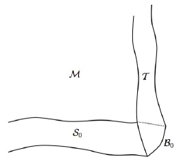
Figure 1: Data on the 3-manifolds ${\cal S}_{0}$ and ${\cal T}$, which intersect in the 2-surface ${\cal B}_{0}$, locally determine a solution in the spacetime manifold ${\cal M}$

.

There are no natural boundaries for the gravitational field analogous to the conducting boundaries that play a major role in electromagnetism. Consequently, the IBVP for Einstein’s equations only received widespread attention after its importance to the artificial outer boundaries used in numerical relativity was pointed out stewart . The first well-posed IBVP was achieved for a tetrad formulation of Einstein’s theory in terms of a first differential order system which included the tetrad, the connection and the curvature tensor as evolution fields fn . A strongly well-posed IBVP was later established for the harmonic formulation of Einstein’s equations as a system of second order quasilinear wave equations for the metric wpgs ; wpe . Strong well-posedness guarantees the existence of a unique solution which depends continuously on both the Cauchy data and the boundary data. The results were further generalized in isol to apply to general quasilinear symmetric hyperbolic systems whose boundary conditions have a certain hierarchical form.

The initial data for the Cauchy problem can be formulated in terms of two symmetric tensor fields $\tilde{h}_{ab}$ (a Euclidean 3-metric) and $\tilde{k}_{ab}$ on a 3-manifold $\tilde{\cal S}_{0}$ subject to the (Hamiltonian and momentum) constraints

$$0={}^{(3)}\tilde{R}+(\tilde{k}^{a}_{a})^{2}-\tilde{k}_{ab}\tilde{k}^{ab}\quad$$ (1)

and

$$0=\tilde{\nabla}_{a}(\tilde{k}^{a}_{b}-\delta^{a}_{b}\tilde{k}^{c}_{c}),$$ (2)

where $\tilde{\nabla}_{a}$ is the covariant derivative and ${}^{(3)}\tilde{R}$ is the curvature scalar associated with $\tilde{h}_{ab}$. As characterized in  hawkel , via an embedding in a 4-dimensional manifold ${\cal M}$, the data $\tilde{h}_{ab}$ and $\tilde{k}_{ab}$ on the disembodied 3-manifold $\tilde{\cal S}_{0}$ determine a Lorentzian metric satisfying Einstein’s equations which is unique up to diffeomorphism and whose restriction to the embedding ${\cal S}_{0}$ of $\tilde{\cal S}_{0}$ gives rise to its intrinsic 3-metric $h_{ab}$ and extrinsic curvature $k_{ab}$.

Here we present an analogous result for the IBVP. The difficulties underlying the IBVP, which have most recently been discussed in juerg and hjuerg , make the formulation of disembodied boundary data more difficult than for the Cauchy problem. There are three main complications.

• The first complication stems from a well-known property of the IBVP for the flat-space scalar wave equation

  $$(\partial_{t}^{2}-\nabla^{2})\Phi=0$$

  in the region $x\leq 0$. Although the initial Cauchy data consist of $\Phi|_{t=0}$ and $\partial_{t}\Phi|_{t=0}$, only half as much boundary data can be freely prescribed at $x=0$, e.g the Dirichlet data $\partial_{t}\Phi|_{x=0}$, or the Neumann data $\partial_{x}\Phi|_{x=0}$ or the Sommerfeld data $(\partial_{t}+\partial_{x})\Phi|_{x=0}$ (based upon the derivative in the outgoing characteristic direction). For a given physical problem, this implies that the boundary data cannot be prescribed before the boundary condition is specified, i.e. the correct boundary data depend upon the boundary condition, unlike the situation for the Cauchy problem. The analogue in the gravitational case is the inability to prescribe both the metric and its normal derivative on a timelike boundary, which implies that you cannot freely prescribe both the intrinsic metric of the boundary and its extrinsic curvature. This leads to a further complication regarding constraint enforcement on the boundary, i.e. the Hamiltonian and momentum constraints (1) and (2) cannot be enforced directly because they couple the metric and its normal derivative. Here we restrict our attention to Sommerfeld boundary data which we prescribe in a constraint free manner.

• A Sommerfeld boundary condition for a metric component supplies the value of the derivative $K^{c}\partial_{c}g_{ab}$ in an outgoing null direction $K^{c}$. Such boundary conditions are very beneficial for numerical work since they allow discretization error to propagate across the boundary (whereas Dirichlet and Neumann boundary conditions reflect the error and trap it in the numerical grid). However, the boundary does not pick out a unique outgoing null direction at a given point (but, instead, essentially a half null cone). This complicates the geometric formulation of a Sommerfeld boundary condition. In addition, constraint preservation does not allow specification of Sommerfeld data for all components of the metric, as will be seen in formulating the Sommerfeld conditions (26) - (28).

• The third major complication arises from gauge freedom. In the evolution of the Cauchy data it is necessary to introduce a foliation of the spacetime by Cauchy hypersurfaces ${\cal S}_{t}$, with unit timelike normal $n_{a}$. The evolution of the spacetime metric

  $$g_{ab}=-n_{a}n_{b}+h_{ab}$$ (3)

  is carried out along the flow of an evolution vector field $t^{a}$ related to the normal by the lapse $\alpha$ and shift $\beta^{a}$ according to

  $$t^{a}=\alpha n^{a}+\beta^{a}\,,\quad\beta^{a}n_{a}=0.$$ (4)

  The choice of foliation is part of the gauge freedom in the resulting solution but does not enter into the specification of the initial data. In the IBVP, the foliation is unavoidably coupled with the formulation of the boundary condition. Thus some gauge information must be incorporated in the formulation of the boundary condition and boundary data.

In order to resolve these complications, we include the specification of a foliation ${\cal B}_{t}$ of the boundary ${\cal T}$ as part of the boundary data. This supplies the gauge information which determines a unique outgoing null direction for a Sommerfeld condition. In Section II, we formulate the 3-dimensional prescription of the boundary data and the statement of our main result, a Theorem establishing the existence of a solution satisfying a version of the geometric uniqueness property proposed in hjuerg . The 3-dimensional description of the data in terms of scalar, vector and tensor fields intrinsic to the boundary is quite abstract at this stage. Their physical significance only becomes clear in Section III, where the proof of the Theorem is given. The proof is based upon the well-posedness of the 4-dimensional geometrical formulation of the harmonic IBVP given in juerg . Constraint preservation is established by incorporating the harmonic conditions into the boundary conditions.

The motivation for this work stems from the need for an improved understanding and implementation of boundary conditions in the computational codes being used to simulate binary black holes. We discuss the applicability of our results to numerical relativity in Sec. IV.

Much of the presentation in the paper is coordinate independent and we use Latin letters $(a,b,c,...)$ as abstract indices wald to denote the types of vector and tensor fields and to indicate their manipulations. This notation serves to describe either 4-dimensional tensor fields on the spacetime ${\cal M}$ or 3-dimensional tensor fields intrinsic to ${\cal S}_{0}$ or ${\cal T}$. When spacetime coordinates $x^{\mu}=(t,x^{i})$ are introduced, we use Greek letters $(\mu,\nu,\rho,...)$ to describe the corresponding 4-dimensional tensor components and Latin letters $(i,j,k,...)$ to denote the spatial components.

II Disembodied data for the IBVP

We state our main result concerning Sommerfeld boundary data for Einstein’s equations.

Geometric Uniqueness Theorem: Consider the 3-manifolds $\tilde{\cal T}$ and $\tilde{\cal S}_{0}$ meeting in an edge $\tilde{\cal B}_{0}$. On $\tilde{\cal S}_{0}$ prescribe the smooth, symmetric tensor fields $\tilde{h}_{ab}$ and $\tilde{k}_{ab}$, subject to the Hamiltonian and momentum constraints and the condition that $\tilde{h}_{ab}$ be a Riemannian metric . On $\tilde{\cal B}_{0}$ prescribe the smooth scalar field $\tilde{\Theta}$. On $\tilde{\cal T}$ prescribe a smooth foliation $\tilde{\cal B}_{t}$ parametrized by a scalar function $\tilde{t}$, where (for convenience) $\tilde{t}=0$ on $\tilde{\cal B}_{0}$. In addition, on $\tilde{\cal T}$, prescribe the scalar field $\tilde{q}$, the vector field $\tilde{q}^{a}$ and the rank-2 symmetric tensor field $\tilde{\sigma}^{ab}$, which are all smooth and vanish on $\tilde{\cal B}_{0}$. Here the rank-2 property of $\tilde{\sigma}^{ab}$ is defined with respect to the foliation $\tilde{\cal B}_{t}$ by the requirement

$$\tilde{\sigma}^{ab}\partial_{a}\tilde{t}=0.$$ (5)

Then, after embedding $\tilde{\cal S}_{0}\cup\tilde{\cal T}$ as the boundary ${\cal S}_{0}\cup{\cal T}$ of a 4-manifold ${\cal M}$, as depicted in Fig. 1, this data provides Sommerfeld boundary data for a vacuum spacetime, in a region including a neighborhood of the embedded edge ${\cal B}_{0}$, which is unique up to diffeomorphism.

The geometrical interpretation of the data involves the metric of the embedded spacetime, whose existence is the content of the Theorem. Before proceeding to the proof in the next section, it is useful to supply some intuitive meaning to the data. As in the Cauchy problem, $\tilde{h}_{ab}$ and $\tilde{k}_{ab}$ are identified with the 3-metric and the extrinsic curvature of the embedding ${\cal S}_{0}$ of $\tilde{\cal S}_{0}$. The scalar field $\tilde{\Theta}$ determines the hyperbolic angle describing the initial velocity of the embedded boundary ${\cal T}$ relative to the inertial frame picked out by ${\cal S}_{0}$. The fields $\tilde{q}$ and $\tilde{q}^{a}$ supply information concerning the subsequent dynamics of the boundary and its foliation. Together $\tilde{q}$ and $\tilde{q}^{a}$ determine the components of a 4-vector $q^{a}$ describing the curvature of the outgoing null geodesics normal in ${\cal M}$ to the embedding ${\cal B}_{t}$ of $\tilde{\cal B}_{t}$. The field $\tilde{\sigma}^{ab}$ determines the optical shear $\sigma$ of the outgoing null hypersurface through ${\cal B}_{t}$.

Note that the data contains no metric information about the embedded boundary ${\cal T}$, not even that it is a timelike 3-manifold. Such structure only emerges from the construction of a solution for the spacetime metric. Thus fields derived algebraically from the metric, such as the unit normal to the boundary, are to be considered as subsidiary unknowns.

The requirement that the boundary data vanish at $\tilde{\cal B}_{0}$ stems from its interpretation relative to the initial Cauchy data. This requirement ensures the continuity of the resulting spacetime metric and its first derivatives. The full compatibility conditions necessary for a $C^{\infty}$ spacetime metric involve enforcing the Einstein equations and their derivatives on ${\cal B}_{0}$. It is not clear how to implement $C^{\infty}$ compatibility conditions in terms of disembodied data.

III The existence of a geometrically unique solution

Our task is to show that harmonic evolution of the data prescribed in the Geometric Uniqueness Theorem of Sec. II locally determine a vacuum spacetime which is unique up to diffeomorphism. We embed $\tilde{\cal S}_{0}$, $\tilde{\cal T}$ and $\tilde{\cal B}_{0}$ in a 4-manifold ${\cal M}$ with boundary consisting of the corresponding pieces ${\cal S}_{0}$, ${\cal T}$ and ${\cal B}_{0}$. The unknown is a spacetime metric $g_{ab}$ on ${\cal M}$ which satisfies Einstein’s equations and is determined up to a diffeomorphism by the data specified in the Theorem. We follow the construction given in juerg .

The first step is to give initial data for $g_{ab}$. Let $h_{ab}$ and $k_{ab}$ be the fields induced by $\tilde{h}_{ab}$ and $\tilde{k}_{ab}$ on ${\cal S}_{0}$; $\Theta$ be the field induced by $\tilde{\Theta}$ on ${\cal B}_{0}$; and $\hat{q}$, $\hat{q}^{a}$ and $\hat{\sigma}^{ab}$ be the fields induced by $\tilde{q}$, $\tilde{q}^{a}$ and $\tilde{\sigma}^{ab}$ on ${\cal T}$. Let ${\cal B}_{t}$ be the foliation of ${\cal T}$ corresponding to the embedding of $\tilde{\cal B}_{t}$, where $t$ is the parametrization induced by $\tilde{t}$. On ${\cal S}_{0}$ prescribe a transverse field $n^{a}$ and construct the Lorentzian metric $g^{ab}=-n^{a}n^{b}+h^{ab}$, so that $n^{a}$ is the future directed unit normal to ${\cal S}_{0}$. Require that $n^{a}$ satisfy $n^{a}N_{a}|_{{\cal B}_{0}}=\sinh\Theta$, where $N_{a}$ is the outward unit normal to ${\cal T}$.

We introduce the boundary decomposition of the metric

$$g_{ab}=N_{a}N_{b}-T_{a}T_{b}+Q_{ab},$$ (6)

where $T_{a}$ is the future directed unit normal in ${\cal T}$ to ${\cal B}_{t}$. (Here the boundary fields $N_{a}$, $T_{a}$ and $Q_{ab}$ are unknowns subsidiary to $g_{ab}$.) This leads to an orthonormal tetrad $(T^{a},N^{a},Q^{a},\bar{Q}^{a})$ on ${\cal T}$, where $Q^{a}$ is a complex null vector tangent to ${\cal B}_{t}$ with normalization

$$Q_{ab}=Q_{(a}\bar{Q}_{b)}\,,\quad Q^{a}\bar{Q}_{a}=2\,,\quad Q^{a}Q_{a}=0.$$ (7)

(The tetrad is unique up to the spin freedom $Q^{a}\rightarrow e^{i\theta}Q^{a}$ which does not enter our construction in any essential way.) Uniquely associated with this tetrad (independent of the choice of $Q^{a}$) are the outgoing and ingoing null vector fields $K^{a}=T^{a}+N^{a}$ and $L^{a}=T^{a}-N^{a}$, respectively, which lie in the null directions normal to ${\cal B}_{t}$. They form a null tetrad $(K^{a},L^{a},Q^{a},\bar{Q}^{a})$ with metric decomposition

$$g_{ab}=-K_{(a}L_{b)}+Q_{(a}\bar{Q}_{b)}.$$ (8)

Next we tie down the gauge freedom by introducing an evolution field $t^{a}$ on ${\cal M}$. We require that $t^{a}$ be tangent to ${\cal T}$ and that it generate the foliation ${\cal B}_{t}$ according to

$${\cal L}_{t}t=1,$$ (9)

where ${\cal L}_{t}$ is the Lie derivative with respect to $t^{a}$. We extend $t^{a}$ to ${\cal M}$ such that it generates a foliation ${\cal S}_{t}$, with parametrization satisfying (9) and unit normal $n^{a}$. The gauge freedom is then pinned down by introducing spatial coordinates $x^{i}$ on ${\cal S}_{0}$ and extending them to ${\cal M}$ according to

$${\cal L}_{t}x^{i}=0.$$ (10)

The scalars $x^{\mu}=(t,x^{i})$ serve as coordinates for ${\cal M}$ which are adapted to the evolution. Note that $t^{a}$ and the adapted coordinates $x^{\mu}$ are explicitly constructed fields on ${\cal M}$ with no metric properties. In the relationship (4) between $t^{a}$ and the unit normal $n^{a}$ to ${\cal S}_{t}$, it is $n^{a}$ which contains metric information and is a subsidiary unknown.

As part of the initial data, we prescribe ${\cal L}_{t}n^{a}$ on ${\cal S}_{0}$. Along with the initial choice of $n^{a}$, $h_{ab}$ and $k_{ab}$, this determines the initial data $g_{ab}|_{t=0}$ and ${\cal L}_{t}g_{ab}|_{t=0}$. We use the evolution field $t^{a}$ to provide a background metric ${\mbox{\em\r{g}\hskip 0.28453pt}}_{ab}$ on ${\cal M}$ which is uniquely and geometrically determined by the Lie transport of the initial data according to

$${\mbox{\em\r{g}\hskip 0.28453pt}}_{ab}|_{t=0}=g_{ab}|_{t=0}\,,\quad{\cal L}_{t}{\mbox{\em\r{g}\hskip 0.28453pt}}_{ab}|_{t=0}={\cal L}_{t}g_{ab}|_{t=0}\,,\quad{\cal L}_{t}{\cal L}_{t}{\mbox{\em\r{g}\hskip 0.28453pt}}_{ab}=0.$$ (11)

In the coordinates $x^{\mu}=(t,x^{i})$ adapted to the evolution, this reduces to

$${\mbox{\em\r{g}\hskip 0.28453pt}}_{\mu\nu}=g_{\mu\nu}|_{t=0}+t(\partial_{t}g_{\mu\nu}|_{t=0}).$$ (12)

The connection $\nabla{}^{\mbox{\r{~}}}{}_{a}$ and curvature tensor $\mbox{\em\r{R}}{}^{d}{}_{cab}$ associated with the background $\mbox{\em\r{g}\hskip 0.28453pt}_{ab}$ have the same transformation properties as the corresponding quantities $\nabla_{a}$ and $R^{d}{}_{cab}$ associated with $g_{ab}$. In particular, the difference $\nabla_{a}-\nabla{}^{\mbox{\r{~}}}{}_{a}$ defines a tensor field $C^{d}_{ab}$ according to

$$(\nabla_{a}-\nabla{}^{\mbox{\r{~}}}{}_{a})v^{d}=C^{d}_{ab}v^{b},$$ (13)

for any vector field $v^{b}$. In terms of the (nonlinear) perturbation

$$f_{ab}=g_{ab}-\mbox{\em\r{g}\hskip 0.28453pt}_{ab}$$ (14)

of the metric from the background, we have

$$C^{d}_{ab}=\frac{1}{2}g^{dc}\left(\nabla{}^{\mbox{\r{~}}}{}_{a}f_{bc}+\nabla{}^{\mbox{\r{~}}}{}_{a}f_{bc}-\nabla{}^{\mbox{\r{~}}}{}_{c}f_{ab}\right).$$ (15)

We take $f_{ab}$ to be the evolution variable for solving Einstein’s equations. Since $\mbox{\em\r{g}\hskip 0.28453pt}_{ab}$ is explicitly known, a solution for $f_{ab}$ is equivalent to a solution for $g_{ab}$. By construction, the initial data for $f_{ab}$ is homogeneous, i.e.

$$f_{ab}|_{t=0}={\cal L}_{t}f_{ab}|_{t=0}=0.$$ (16)

The boundary data on ${\cal T}$ consist of the vector field

$$q^{a}=\hat{q}N^{a}+\hat{q}^{a}$$ (17)

and the tensor field

$$\sigma^{ab}=\hat{\sigma}^{ab}-\frac{1}{2}Q^{ab}Q_{cd}\hat{\sigma}^{cd}.$$ (18)

Here, and elsewhere, the physical metric $g_{ab}$ is used to raise and lower indices and to normalize the tetrad vectors.

Now, just as the Cauchy data $h_{ab}$ and $k_{ab}$ must be identified as the intrinsic metric and extrinsic curvature of ${\cal S}_{0}$ in order to construct a solution of the initial value problem, we give a geometric identification of the boundary data. We identify this data as the geodesic curvature and shear, relative to their background metric values, of the outgoing null vector $K^{a}$ on ${\cal T}$ according to the formulae

$$q^{a} = K^{b}(\nabla_{b}-\nabla{}^{\mbox{\r{~}}}{}_{b})K^{a},$$ (19)

$$\sigma^{ab} = \frac{1}{2}(Q^{ac}Q^{bd}-\frac{1}{2}Q^{ab}Q^{cd})(\nabla_{c}-\nabla{}^{\mbox{\r{~}}}{}_{c})K_{d}.$$ (20)

The last equation can be re-expressed in the spin-weight-2 form

$$\sigma:=Q^{a}Q^{b}\sigma_{ab}=\frac{1}{2}Q^{a}Q^{b}(\nabla_{a}-\nabla{}^{\mbox{\r{~}}}{}_{a})K_{b}.$$ (21)

The use of the shear in posing geometrical boundary conditions for the harmonic formulation was suggested earlier in ruiz .

Using (13) and (15), we recast (19) and (21) as Sommerfeld boundary conditions which determine the components of the outgoing null derivatives $K^{a}\nabla{}^{\mbox{\r{~}}}{}_{a}f_{bc}$ according to

$$\frac{1}{2}K^{b}K^{c}K^{a}\nabla{}^{\mbox{\r{~}}}{}_{a}f_{bc} = q^{a}K_{a},$$ (22)

$$(Q^{b}K^{c}K^{a}-\frac{1}{2}K^{b}K^{c}Q^{a})\nabla{}^{\mbox{\r{~}}}{}_{a}f_{bc} = q^{a}Q_{a},$$ (23)

$$(L^{b}K^{c}K^{a}-\frac{1}{2}K^{b}K^{c}L^{a})\nabla{}^{\mbox{\r{~}}}{}_{a}f_{bc} = q^{a}L_{a},$$ (24)

$$(\frac{1}{2}Q^{b}Q^{c}K^{a}-Q^{b}K^{c}Q^{a})\nabla{}^{\mbox{\r{~}}}{}_{a}f_{bc} = 2\sigma.$$ (25)

In addition to these six Sommerfeld conditions, we impose the four additional boundary conditions that ${\cal C}^{d}:=g^{ab}C^{d}_{ab}=0$ on ${\cal T}$, i.e. the harmonic constraints. In terms of the null tetrad decomposition, they take the Sommerfeld form

$$-2{\cal C}^{a}K_{a}=\left(Q^{b}\bar{Q}^{c}K^{a}+K^{b}K^{c}L^{a}-K^{b}\bar{Q}^{c}Q^{a}-K^{b}Q^{c}\bar{Q}^{a}\right)\nabla{}^{\mbox{\r{~}}}{}_{a}f_{bc} = 0,$$ (26)

$$-2{\cal C}^{a}Q_{a}=\left(L^{b}Q^{c}K^{a}+K^{b}Q^{c}L^{a}-K^{b}L^{c}Q^{a}+Q^{b}Q^{c}\bar{Q}^{a}\right)\nabla{}^{\mbox{\r{~}}}{}_{a}f_{bc} = 0,$$ (27)

$$-2{\cal C}^{a}L_{a}=\left(L^{b}L^{c}K^{a}+Q^{b}\bar{Q}^{c}L^{a}-\bar{Q}^{b}L^{c}Q^{a}-Q^{b}L^{c}\bar{Q}^{a}\right)\nabla{}^{\mbox{\r{~}}}{}_{a}f_{bc} = 0.$$ (28)

Together, (22) - (28) provide Sommerfeld boundary conditions for the components of $K^{a}\nabla{}^{\mbox{\r{~}}}{}_{a}f_{bc}$ in the sequential order $(KK),(QK),(LK),(QQ),(Q\bar{Q}),(LQ),(LL)$ in terms of the boundary data and the derivatives of preceding components in the sequence. Such a hierarchy of Sommerfeld boundary conditions satisfy the requirements of Theorem 1 of isol which establishes a strongly well-posed IBVP for a quasilinear hyperbolic system.

In order to apply this theorem, we reduce Einstein’s equations to a quasilinear wave system by modifying the Einstein tensor by the harmonic constraints

$${\cal C}^{d}=g^{ab}C^{d}_{ab}=\frac{1}{2}g^{ab}g^{dc}\left(\nabla{}^{\mbox{\r{~}}}{}_{a}f_{bc}+\nabla{}^{\mbox{\r{~}}}{}_{a}f_{bc}-\nabla{}^{\mbox{\r{~}}}{}_{c}f_{ab}\right)$$ (29)

according to

$$E^{ab}:=G^{ab}-\nabla^{(a}{\cal C}^{b)}+\frac{1}{2}g^{ab}\nabla_{d}{\cal C}^{d}.$$ (30)

We eliminate the coordinate freedom, up to our choice of evolution field $t^{a}$ on ${\cal M}$ and coordinates $x^{i}$ on ${\cal S}_{0}$, by working in the coordinates $x^{\mu}$ adapted to the evolution. The coordinate components of (29) then take the form

$${\cal C}^{\rho}=\frac{1}{2}g^{\mu\nu}g^{\rho\sigma}\left(\nabla{}^{\mbox{\r{~}}}{}_{\mu}f_{\nu\sigma}+\nabla{}^{\mbox{\r{~}}}{}_{\mu}f_{\nu\sigma}-\nabla{}^{\mbox{\r{~}}}{}_{\sigma}f_{\mu\nu}\right)=g^{\mu\nu}(\Gamma^{\rho}_{\mu\nu}-\Gamma{}^{\mbox{\r{~}}}{}^{\rho}_{\mu\nu}).$$ (31)

The requirement that $\Gamma^{\rho}:=g^{\mu\nu}\Gamma^{\rho}_{\mu\nu}=0$ is the standard harmonic coordinate condition that $\Box_{g}x^{\mu}=0$. In the present case, setting ${\cal C}^{\rho}=0$ implies $\Gamma^{\rho}=g^{\mu\nu}\Gamma{}^{\mbox{\r{~}}}{}^{\rho}_{\mu\nu}$, which is an example of harmonic coordinates with a forcing term, as discussed in Friedrich . (In numerical relativity, these have been called generalized harmonic coordinates pret .) For more general forcing terms the harmonic constraint takes the form

$$\Gamma^{\rho}=H^{\rho}(x,g),$$ (32)

where restriction of the forcing term $H^{\rho}$ to depend only upon $x^{\mu}$and $g_{\mu\nu}$ ensures that the system remains well-posed.

In the adapted coordinates, the reduced Einstein equations $E_{\mu\nu}=0$ form the desired quasilinear wave system for $f_{\mu\nu}$,

$$g^{\rho\sigma}\nabla{}^{\mbox{\r{~}}}{}_{\rho}\nabla{}^{\mbox{\r{~}}}{}_{\sigma}f_{\mu\nu}=2g_{\lambda\tau}g^{\rho\sigma}C^{\lambda}{}_{\mu\rho}C^{\tau}{}_{\nu\sigma}+4C^{\rho}{}_{\sigma(\mu}g_{\nu)\lambda}C^{\lambda}{}_{\rho\tau}g^{\sigma\tau}-2g^{\rho\sigma}\mbox{\em\r{R}}^{\lambda}{}_{\rho\sigma(\mu}g_{\nu)\lambda}.$$ (33)

With the hierarchy of Sommerfeld boundary conditions (22) - (28), Theorem 1 of isol now applies and ensures that (33) has a well-posed IBVP and, in particular, determines a unique solution $f_{\mu\nu}$. In addition, the resulting metric $g_{\mu\nu}$ must satisfy the harmonic constraints ${\cal C}^{\rho}=0$ because they are built into the initial data and boundary conditions. (See Sec. IV for details concerning constraint preservation.) Therefore $g_{\mu\nu}$ solves Einstein’s equations.

The solution has been obtained in coordinates which are harmonic with respect to the background $\mbox{\em\r{g}\hskip 0.28453pt}_{\mu\nu}$, i.e. $g^{\mu\nu}(\Gamma^{\rho}_{\mu\nu}-\Gamma{}^{\mbox{\r{~}}}{}^{\rho}_{\mu\nu})=0$. The resulting spacetime metric $g_{ab}$ and background metric $\mbox{\em\r{g}\hskip 0.28453pt}_{ab}$ determined by the data are in a gauge which depends upon the choice of evolution field $t^{a}$. Under a diffeomorphism $\Psi$ of ${\cal M}$ which reduces to the identity map on ${\cal S}_{0}$ and ${\cal T}$, we have $(t^{a},g_{ab},\mbox{\em\r{g}\hskip 0.28453pt}_{ab})\rightarrow(\Psi_{*}t^{a},\Psi^{*}g_{ab},\Psi^{*}\mbox{\em\r{g}\hskip 0.28453pt}_{ab})$. Thus $\Psi^{*}g_{ab}$ is a diffeomorphic solution of Einstein’s equations which is harmonic with respect to the background $\Psi^{*}\mbox{\em\r{g}\hskip 0.28453pt}_{ab}$.

A more important question, which concerns the issue of geometric uniqueness raised in hjuerg , is the behavior of the spacetime under a diffeomorphism $\tilde{\Psi}$ of the disembodied boundary $\tilde{\cal T}$. It is known for the Cauchy problem that data $(\tilde{\Psi}^{*}\tilde{h}_{ab},\tilde{\Psi}^{*}\tilde{k}_{ab})$ on $\tilde{\cal S}_{0}$ lead to a spacetime which is isometric to the spacetime with Cauchy data $(\tilde{h}_{ab},\tilde{k}_{ab})$. The analogous result holds for the boundary data. Under a diffeomorphism $\tilde{\Psi}$ of $\tilde{\cal T}$ the boundary data maps according to $(\tilde{t},\tilde{q},\tilde{q}^{ab},\tilde{\sigma}^{ab})\rightarrow(\tilde{\Psi}^{*}\tilde{t},\tilde{\Psi}^{*}\tilde{q},\tilde{\Psi}_{*}\tilde{q}^{ab},\tilde{\Psi}_{*}\tilde{\sigma}^{ab})$. After the embedding in ${\cal M}$, this induces data $(\tilde{\Psi}^{*}t,\tilde{\Psi}^{*}\hat{q},\tilde{\Psi}_{*}\hat{q}^{ab},\tilde{\Psi}_{*}\hat{\sigma}^{ab})$ on ${\cal T}$. Now consider any smooth extension of $\tilde{\Psi}$ to a diffeomorphism of ${\cal M}$. Suppose the original data leads by the above construction to the spacetime metric $g_{ab}$ with the evolution field $t^{a}$, background $\mbox{\em\r{g}\hskip 0.28453pt}_{ab}$ and relative geodesic curvature and relative shear $(q^{a},\sigma^{ab})$ of the outgoing null vector $K^{a}$ normal to the $t$-foliation of ${\cal T}$. Then, by the same construction, the mapped data lead to the metric $\tilde{\Psi}^{*}g_{ab}$ with the evolution field $\tilde{\Psi}_{*}t^{a}$, background $\tilde{\Psi}^{*}\mbox{\em\r{g}\hskip 0.28453pt}_{ab}$ and relative geodesic curvature and relative shear $(\tilde{\Psi}_{*}q^{a},\tilde{\Psi}_{*}\sigma^{ab})$ of the outgoing null vector $\tilde{\Psi}_{*}K^{a}$ normal to the $\tilde{\Psi}^{*}t$-foliation of ${\cal T}$. In this way, diffeomorphisms of $\tilde{\cal S}$ and $\tilde{\cal T}$, which map their intersection $\tilde{\cal B}_{0}$ into itself, generate an isometry class of vacuum spacetimes.

We have thus shown that the resulting vacuum spacetimes are diffeomorphic if the disembodied boundary data and initial Cauchy data are diffeomorphic. This comprises a version of geometric uniqueness, which has been pointed out as a missing ingredient in prior formulations of the IBVP hjuerg . However, the result is not as strong as for the pure Cauchy problem for which the converse is also true: the resulting vacuum spacetimes are diffeomorphic only if the initial data are diffeomorphic. The converse is more complicated for the IBVP and does not hold in the disembodied setting because the data $\tilde{\sigma}^{ab}$ are superfluous. It is only the trace-free part of the embedded data $\hat{\sigma}^{ab}$ which enters the shear $\sigma^{ab}$. But there is no way to pick out the trace free part without knowledge of the metric, which is an unknown at the stage of specifying data. (For linear perturbations, a background metric could be used but this construction does not extend to the nonlinear case.) This is perhaps an unavoidable feature of disembodied Sommerfeld data for the IBVP.

As a result, disembodied boundary data which are not related by a diffeomorphism can lead to isometric spacetimes. However, it follows by direct geometrical construction that an isometry class of spacetimes does uniquely determine the embedded boundary data $q^{a}$ and $\sigma^{ab}$ up to a diffeomorphism. It is only upon the transition from $\sigma^{ab}$ to $\hat{\sigma}^{ab}$ that the ambiguity of adding a trace enters. In this sense, a stronger version of geometric uniqueness applies to the embedded data.

The Sommerfeld boundary conditions were based upon the background metric obtained by the Lie transport (11) of the Cauchy data along the streamlines of $t^{a}$. Modification of this transport law would lead to a different background and the spacetime generated by the same disembodied data would in general not be diffeomorphic. This is similar to the scalar wave problem, for which the same boundary data would lead to different solutions if, say, a Dirichlet boundary condition were used instead of a Sommerfeld condition. In the present case, a new background metric implies a different form of the Sommerfeld condition and, for fixed boundary data, the resulting spacetime will (in general) not be isometric to the original spacetime. The effect of the boundary data is changed by the difference between the two background connections.

IV Numerical application

The motivation for this work has been the treatment of the outer boundary in the numerical simulation of the inspiral and merger of binary black holes. The boundary conditions (22) - (28), which lead to a strongly well-posed IBVP, can be applied directly to any of the harmonic evolution codes which have been used to simulate this binary problem fP05 ; fP06 ; lLmSlKrOoR06 ; oRlLmS07 ; bSdPlRjTjW07 . At present, none of these harmonic codes incorporate boundary conditions that ensure strong well-posedness. The closest example is the pseudo-spectral harmonic code described in lLmSlKrOoR06 ; oRlLmS07 which incorporates a second differential order boundary condition which freezes the $\Psi_{0}$ Weyl component and was shown to be well-posed in the generalized sense in the high frequency limit ruiz .

An important attribute of strong well-posedness is the estimate of the boundary values of the solution and its derivatives which are provided by an energy conservation law obeyed by the principle part of the equations. This boundary stability extends to the semi-discrete system of ordinary differential equations in time which are obtained by replacing spatial derivatives by finite differences obeying summation by parts (the discrete counterpart of integration by parts), so that energy conservation caries over to the semi-discrete problem. This stability then extends to the numerical evolution algorithm obtained by applying an appropriate time integrator, such as Runge-Kutta.

The advantage of boundary stability in numerical applications is that the smoothness of the solution is unaffected by reflections off the boundary. This avoids the long timescale instabilities which might otherwise arise from multiple reflections. For the harmonic Einstein problem, each component of the metric obeys a quasilinear wave equation so that it is straightforward to develop a summation by parts algorithm based upon the standard energy expression for a scalar wave in a curved spacetime mBbSjW06 . A code incorporating such an algorithm was applied, using a version of the well-posed Sommerfeld boundary conditions presented here, to the test problem of a highly nonlinear gauge wave propagating inside a cubic boundary mBhKjW07 . Although the proof of strong well-posedness given in wpe was based upon a scalar wave energy differing by a small boost from the standard energy expression, the successful results for this test problem confirm the robustness of the underlying approach.

Strong well-posedness extends to more general quasi-harmonic formulations for which the reduced Einstein equations have the form

$$E^{\mu\nu}:=G^{\mu\nu}-\nabla^{(\mu}{\cal C}^{\nu)}+\frac{1}{2}g^{\mu\nu}\nabla_{\rho}{\cal C}^{\rho}+A^{\mu\nu}_{\sigma}{\cal C}^{\sigma}=0,$$ (34)

where ${\cal C}^{\rho}=g^{\mu\nu}\Gamma^{\rho}_{\mu\nu}-H^{\rho}(x,g)$ are the generalized harmonic constraints (32) and the coefficients $A^{\mu\nu}_{\sigma}$ have the dependence $A^{\mu\nu}_{\sigma}(x,g,\partial g)$. (This includes constraint modified versions of the harmonic system.) Constraint preservation follows from the Bianchi identity $\nabla_{\mu}G^{\mu\nu}=0$ which implies a homogeneous wave equation for ${\cal C}^{\mu}$,

$$\nabla^{\rho}\nabla_{\rho}\,{\cal C}^{\mu}+R^{\mu}_{\rho}\,{\cal C}^{\rho}-2\nabla_{\rho}(A^{\mu\rho}_{\sigma}{\cal C}^{\sigma})=0.$$ (35)

If the boundary conditions enforce ${\cal C}^{\rho}|_{\cal T}=0$ and the initial data enforces ${\cal C}^{\rho}|_{{\cal S}_{0}}=\partial_{t}{\cal C}^{\rho}|_{{\cal S}_{0}}=0$ then the unique solution of (35) is ${\cal C}^{\rho}=0$. As a result, the Sommerfeld boundary conditions in the geometrical form (22) - (25), along with (26) - (28) which enforce ${\cal C}^{\rho}|_{\cal T}=0$, lead to a well-posed harmonic IBVP in which the harmonic constraints ${\cal C}^{\rho}=0$ are satisfied everywhere. In turn, (34) implies that the Hamiltonian and momentum constraints $G^{\mu\nu}n_{\nu}=0$ are also satisfied.

Beyond the geometrical aspects of the harmonic IBVP, there are practical concerns that arise in astrophysical applications. The linear time dependence of the background metric (12) could lead to deleterious long time scale effects in numerical simulations. For that reason, it is preferable to modify the prescription (11) for the background metric so that (12) changes to

$${\mbox{\em\r{g}\hskip 0.28453pt}}_{\mu\nu}=g_{\mu\nu}|_{t=0}+te^{-\lambda t}(\partial_{t}g_{\mu\nu}|_{t=0})$$ (36)

and the time dependence damps on a time scale determined by $\lambda$. Alternatively, the purpose of tying the background metric to the initial Cauchy data was to make clear that it did not affect the geometric uniqueness of the solution. Otherwise, the Minkowski metric in the coordinates adapted to the evolution could have been chosen as the background metric. This would leave intact the well-posedness of the IBVP and might be the most expedient approach in some numerical applications, although (36) has the advantage of suppressing nonlinear effects in the early stage of an evolution.

Another practical concern is that the proper boundary data $q^{a}$ and $\sigma$ are not normally known in an astrophysical application. The practice in simulating an isolated system is to assume homogeneous data on the artificial outer boundary, i.e. $q^{a}=\sigma=0$. Such homogeneous data in general leads to some spurious back reflection from the boundary. However, as discussed in isol for the harmonic IBVP, similar boundary conditions on a round spherical outer boundary of large surface area radius $R$ lead to reflected waves whose amplitude falls off asymptotically as $1/R^{3}$ for both quadrupole gauge waves and quadrupole gravitational waves. (The calculation assumes that the linearized approximation is applicable. Modifications of the boundary conditions by lower differential order terms involving factors of $R$ lead to a faster $1/R^{4}$ falloff for the reflected quadrupole gravitational waves. isol )

The boundary conditions (22) - (28) are slightly different than those considered in isol and, in particular, the homogeneous boundary condition $\sigma=0$ leads to reflected waves with only a $1/R^{2}$ falloff, as previously noted in ruiz . However, improved performance can be obtained by taking advantage of the sensitivity of the boundary conditions to the location of the indices. If (21) and (25) are replaced by

$$2\sigma=\frac{1}{2}Q^{a}Q^{b}(\nabla_{a}-\nabla{}^{\mbox{\r{~}}}{}_{a})K_{b}+\frac{1}{2}Q^{a}Q_{b}(\nabla_{a}-\nabla{}^{\mbox{\r{~}}}{}_{a})K^{b}=\frac{1}{2}(Q^{b}Q^{c}K^{a}-Q^{b}K^{c}Q^{a})\nabla{}^{\mbox{\r{~}}}{}_{a}f_{bc},$$ (37)

then agreement with the corresponding boundary condition (94) of isol is obtained. In that case, for the boundary conditions (22) - (24) and (37), along with the harmonic constraints (26) - (28), the amplitudes of the reflected quadrupole gauge waves and quadrupole gravitational waves again fall off asymptotically as $1/R^{3}$. Thus the application of these Sommerfeld boundary conditions with homogeneous data results in small back reflection from the boundary of an isolated system.

While the Sommerfeld boundary conditions considered here were developed for the harmonic IBVP, their geometric nature allows them to be formally applied to any metric version of the reduced Einstein equations, in particular the alternative “$3+1$” formulations upon which much numerical work has been based. However, in that case, well-posedness and constraint preservation do not necessarily follow. One approach to dealing with these issues would be to re-express the $3+1$ formulations in terms of the covariant 4-dimensional $Z4$ theory z4 ; z4sb , in which the reduced evolution equations take the form (34) but with the harmonic constraints ${\cal C}^{\mu}$ replaced by a more general vector field $Z^{\mu}$, which can be used to change the principle part of the resulting evolution system. The $Z4$ formalism has been shown to encompass the standard $3+1$ formulations, including the Arnowitt-Deser-Misner (ADM) adm , the Kidder-Scheel-Teukolsky kst , the Nagy-Ortiz-Reula nor and the Baumgarte-Shapiro-Shibata-Nakamura (BSSN) bssn1 ; bssn2 formulations. It is possible that the close analogue between the $Z4$ and harmonic formulations might be used to shed light on the analytic properties of $3+1$ systems. However, such an investigation of the well-posedenss of the $3+1$ IBVP is stymied by the fact that none of the systems used in numerical applications have been shown to be symmetric hyperbolic. Some $3+1$ systems have been show to be strongly hyperbolic, which ensures a well-posed Cauchy problem, but symmetric hyperbolicity is required to apply the standard theorems for a well-posed IBVP. For that reason, the discussion here is restricted to how the Sommerfeld boundary conditions developed here might be applied in a manner consistent with what is presently known about $3+1$ formulations.

The boundary conditions (22) - (25) can be translated in a straightforward way into a “3+1” decomposition $x^{\mu}=(t,x^{i})=(t,x,y.z)$, in which the metric takes the form (3) where, in terms of the lapse and shift (4),

$$g_{tt}=-\alpha^{2}+h_{ij}\beta^{i}\beta^{j}\,,\quad g_{ti}=h_{ij}\beta^{j}\,,\quad g_{ij}=h_{ij}.$$ (38)

Although there is a different decomposition (6) intrinsic to the boundary, the outgoing null direction used in formulating a Sommerfeld condition is intrinsic to both decompositions. Let $\hat{N}^{\mu}$ be the unit normal to the boundary foliation ${\cal B}_{t}$, which lies in the $t=const$ Cauchy hypersurface, so that the metric (3) has the further decomposition

$$g_{\mu\nu}=-n_{\mu}n_{\nu}+\hat{N}_{\mu}\hat{N}_{\nu}+Q_{\mu\nu},$$ (39)

where again $Q_{\mu\nu}=Q_{(\mu}\bar{Q}_{\nu)}$ is the 2-metric intrinsic to the foliation ${\cal B}_{t}$ of the boundary. Then the outgoing null vector $K^{\mu}$ normal to the foliation has components $K^{\mu}=T^{\mu}+N^{\mu}=e^{-\Theta}(n^{\mu}+\hat{N}^{\mu})$ where $\Theta$ is the hyperbolic angle arising from the velocity of the boundary relative to the Cauchy hypersurfaces. In terms of the lapse and normal component of the shift,

$$\tanh\Theta=-\frac{1}{\alpha}\beta^{i}\hat{N}_{i},$$ (40)

where $\beta^{i}\hat{N}_{i}<0$ for a boundary which is moving inward with respect to the Cauchy hypersurfaces. The sign of $\beta^{i}\hat{N}_{i}$ determines whether the advective derivative $n^{\mu}\partial_{\mu}$ is outward ($\beta^{i}\hat{N}_{i}<0$) or inward ($\beta^{i}\hat{N}_{i}>0$) at the boundary and, as a result, can affect the number of required boundary conditions.

The Sommerfeld derivative takes the simple 3+1 form

$$K^{\mu}\partial_{\mu}=e^{-\Theta}(n^{\mu}\partial_{\mu}+\hat{N}^{\mu}\partial_{\mu}),\quad\quad\hat{N}^{\mu}\partial_{\mu}=\hat{N}^{i}\partial_{i},$$ (41)

where $n^{\mu}\partial_{\mu}$ is the part containing the time derivative $\partial_{t}$. Thus the Sommerfeld boundary conditions (22) - (25) can be used to supply boundary values for the time derivatives of 6 metric components, or equivalently to supply boundary values for 5 components of the extrinsic curvature $k_{\mu\nu}$ of the Cauchy foliation and for the time derivative of one metric component. In particular, (22) - (23) and (25) supply boundary values for $\hat{N}^{\mu}\hat{N}^{\nu}k_{\mu\nu}$, $Q^{\mu}\hat{N}^{\nu}k_{\mu\nu}$ and $Q^{\mu}Q^{\nu}k_{\mu\nu}$ and (24) supplies the boundary value for the time derivative of the normal component of the shift $\hat{N}_{i}\partial_{t}\beta^{i}$, i.e. $(h^{zz})^{-1/2}\partial_{t}\beta^{z}$ for a boundary aligned with the $z$-coordinate.

The remaining Sommerfeld boundary conditions (26) - (28), which enforce the harmonic constraints, require modification depending upon the particular $3+1$ formulation and gauge conditions. Only 6 components of Einstein’s equations are used in a $3+1$ evolution, with the gauge conditions determining the evolution of the lapse and shift. As a first example, consider the ADM formulation in which the 6 Einstein equations

$$h_{\mu}^{\rho}h_{\nu}^{\sigma}R_{\rho\sigma}=0$$ (42)

are evolved. The evolution of the Hamiltonian and momentum constraints $H:=G_{\mu\nu}n^{\mu}n^{\nu}$ and $P^{\mu}:=h^{\mu\nu}n^{\gamma}G_{\nu\gamma}$ is governed by the contracted Bianchi identity $\nabla_{\nu}G_{\mu}^{\nu}=0$, which gives rise to the symmetric hyperbolic constraint propagation system

$$n^{\gamma}\partial_{\gamma}H-\partial_{j}P^{j} = B^{\gamma}G_{\nu\gamma}n^{\nu}$$ (43)

$$n^{\gamma}\partial_{\gamma}P^{i}-h^{ij}\partial_{j}H = B^{i\gamma}G_{\nu\gamma}n^{\nu},$$ (44)

where the coefficients $B^{\gamma}$ and $B^{\mu\gamma}$ arise from Christoffel symbols and do not enter the principle part. An analysis of this system shows that only one boundary condition is allowed provided $\beta^{i}\hat{N}_{i}\leq 0$, i.e provided the boundary is moving inward relative to the Cauchy hypersurfaces. The theory of symmetric hyperbolic systems then guarantees that all the constraints will be preserved if

$$H+P^{i}N_{i}=G_{\mu\nu}n^{\mu}K^{\nu}=0$$ (45)

is satisfied at the boundary. (Additional boundary conditions are necessary for constraint preservation if $\beta^{i}\hat{N}_{i}>0$.) By combining the evolution system (42) with (45), this boundary condition is equivalent to

$$G_{\mu\nu}K^{\mu}K^{\nu}=0,$$ (46)

i.e. the Raychaudhuri equation (cf. wald )

$$K^{\mu}\partial_{\mu}\theta+\frac{1}{2}\theta^{2}+\sigma\bar{\sigma}=0,$$ (47)

where $\theta=Q^{\mu\nu}\nabla_{\mu}K_{\nu}$ is the expansion of the outgoing null rays tangent to $K^{\mu}$. Thus, for the ADM system, constraint preservation can be enforced by the Sommerfeld boundary condition (47) for $\theta$, which supplies the boundary values for the remaining component $Q^{\mu\nu}k_{\mu\nu}$ of the extrinsic curvature. Unfortunately, although the subsidiary constraint system is symmetric hyperbolic, the ADM evolution system is only weakly hyperbolic and consequently leads to unstable evolution.

In terms of astrophysical applications, the most important $3+1$ formulation is the BSSN system, which has been used by the majority of groups mCcLpMyZ06 ; jBjCdCmKjvM06b ; pDfHdPeSeSrTjTjV06 ; jGetal07 ; bssnsom carrying out binary black hole and neutron star simulations. The development of the BSSN formulation has proceeded through an interplay between educated guesses and feedback from code performance. Only in hindsight has its success spurred mathematical analysis, which has shown that certain versions are strongly hyperbolic and thus have a well-posed Cauchy problem sartig ; nor ; gundl1 . Although significant progress has been made in establishing some of the necessary conditions for well-posedness and constraint preservation of the IBVP gundl2 ; horst ; fritgom ; nunsar , there is still no satisfactory mathematical theory on which to base numerical work. In current numerical practice, the boundary conditions for BSSN evolution systems are applied in a naive, homogeneous Sommerfeld form to each evolution variable (cf. bssnsom ).

The geometric nature of the Sommerfeld boundary conditions (22) - (25) and their role in a well-posed harmonic IBVP suggest that they might lead to improved performance over the present boundary treatment of the BSSN system. However, there are two complications. The first involves the sign of the normal component of the shift $\beta^{i}\hat{N}_{i}$ at the boundary, which also entered the above discussion of the ADM constraint system. A recent analysis nunsar of the BSSN evolution system shows that the number of incoming fields at the boundary, and therefore the number of required boundary conditions, depends upon the sign of $\beta^{i}\hat{N}_{i}$. A practical scheme for dealing with this would require the Dirichlet boundary condition $\beta^{i}\hat{N}_{i}=0$ (or some similar Dirichlet condition to control the sign) rather than the Sommerfeld condition (24) for the normal component of the shift.

The other complication for the BSSN system involves constraint preservation. The BSSN evolution system enforces the 6 Einstein equations

$$h_{\mu}^{\rho}h_{\nu}^{\sigma}R_{\rho\sigma}-\frac{2}{3}h_{\mu\nu}H=0,$$ (48)

for which the constraint system implied by the Bianchi identity takes the form

$$n^{\gamma}\partial_{\gamma}H-\partial_{j}P^{j} = B^{\gamma}G_{\nu\gamma}n^{\nu}$$

$$n^{\gamma}\partial_{\gamma}P^{i}+\frac{1}{3}h^{ij}\partial_{j}H = B^{i\gamma}G_{\nu\gamma}n^{\nu}.$$ (49)

This is no longer symmetric hyperbolic and would not lead to stable constraint preservation even for the Cauchy problem. In order to remedy this, the BSSN evolution system modifies (48) by mixing in a set of auxiliary constraints, which combine with the constraint system (49) to form a larger symmetric hyperbolic constraint system. The freedom in the constraint-mixing parameters and gauge conditions complicates a general treatment. Here the discussion will be limited to a particular choice nunsar for which the linearization off Minkowski space leads to a symmetric hyperbolic system with a well-posed IBVP for the case of a Dirichlet boundary condition $\beta^{i}\hat{N}_{i}=0$ on the normal component of the shift. Although the nonlinear evolution system is no longer symmetric hyperbolic, the boundary conditions for the linearized theory can be formally applied and lead to a symmetric hyperbolic constraint system. Constraint preservation then follows for the parameter range $(b_{1}\leq 1,b_{2}\leq 1)$ in the boundary conditions given in equation (97) of nunsar . The particular choice $b_{1}=0$, leads to the boundary condition pc

$$H-3P^{i}N_{i}=G_{\mu\nu}n^{\mu}(n^{\nu}-3N^{\nu})={\cal Z},$$ (50)

where ${\cal Z}$ represents contributions from the auxiliary constraints, or, by using the evolution system (48),

$$G_{\mu\nu}L^{\mu}L^{\nu}={\cal Z}.$$ (51)

It is a bizarre feature of the $3+1$ problem that the constraint preserving boundary conditions switch from the outgoing Raychaudhuri form (46) to the ingoing Raychaudhuri form (51) in going from the ADM to the BSSN system. The Raychaudhuri equation for the outgoing null direction cannot be imposed in the allowed range of $(b_{1},b_{2})$. Nevertheless, (51) can still be used to supply boundary values for the remaining $Q^{\mu\nu}k_{\mu\nu}$ component of extrinsic curvature.

It appears from the above discussion that the formal application of the Sommerfeld boundary conditions to the BSSN system must be restricted to (22), (23) and (25) which supply boundary values for 5 components of the extrinsic curvature. Boundary values for the remaining $Q^{\mu\nu}k_{\mu\nu}$ component must be obtained in accord with constraint preservation, e.g. from (51 ) or some variant depending upon the particular formulation. The normal component of the shift requires a Dirichlet boundary condition that determines its sign, e.g. $\beta^{i}N_{i}=0$. Appropriate boundary conditions for the lapse and tangential components of the shift depend upon the specific gauge conditions (see nunsar for an example). In the spirit of the BSSN formalism, computational experiments would be necessary to determine whether (22), (23) and (25) lead to improved performance.

V Summary

We have shown that a geometrically unique spacetime can be locally constructed from Sommerfeld data determined by the fields $(\tilde{t},\tilde{q},\tilde{q}^{a},\tilde{\sigma}^{ab})$ on a disembodied boundary $\tilde{\cal T}$, along with the initial data prescribed on ${\tilde{S}}_{0}$. The boundary data specify a foliation $\tilde{\cal B}_{t}$ of $\tilde{\cal T}$ but involve no metric or other geometric properties of the boundary. After the embedding of $\tilde{\cal T}\cup{\tilde{S}}_{0}$ as the boundary ${\cal T}\cup{\cal S}_{0}$ of a 4-manifold ${\cal M}$, the induced fields $(t,\hat{q},\hat{q}^{a},\hat{\sigma}^{ab})$ supply the necessary boundary data for an isometry class of spacetime metrics which satisfy Einstein’s equations. Under diffeomorphisms of the disembodied boundary $\tilde{\cal T}$ and Cauchy hypersurface $\tilde{\cal S}_{0}$, the mapped data determine diffeomorphic vacuum spacetimes.

The gauge in which a particular metric $g_{ab}$ is constructed via a solution of the harmonic IBVP depends upon the choice of evolution field $t^{a}$, which also determines an associated background metric $\mbox{\em\r{g}\hskip 0.28453pt}_{ab}$ by Lie transport of the initial data. Together $g_{ab}$ and $\mbox{\em\r{g}\hskip 0.28453pt}_{ab}$ supply the geometric interpretation of the boundary data in terms of the outgoing null vector $K^{a}$ normal to the foliation ${\cal B}_{t}$ of the boundary. The field $q^{a}$, constructed from $\hat{q}$ and $\hat{q}^{a}$ via (17), is the geodesic curvature of $K^{a}$, relative to its geodesic curvature computed with the background metric. The field $\sigma^{ab}$ (or equivalently $\sigma$) computed from $\hat{\sigma}^{ab}$ via (20) (or (21)) is the shear of $K^{a}$, relative to its background value. The resulting metric is harmonic with respect to the background metric, according to ${\cal C}^{\rho}=0$ (see (31)). All possible choices of $t^{a}$ are related by diffeomorphism, so that all possible gauges are included.

The Sommerfeld boundary conditions have direct application to harmonic evolution codes used in simulating binary black holes, where they would provide a numerical algorithm based upon a strongly well-posed IBVP. Furthermore, for harmonic evolution, homogeneous Sommerfeld data gives rise to asymptotically small back reflection of quadrupole waves from an asymptotically large spherical outer boundary of an isolated system.

The geometric nature of the 6 boundary conditions (22) - (25) suggests that they might also be applicable to codes based upon a $3+1$ formulation, e.g. the BSSN system, as a way to reduce spurious boundary effects generated by the naive Sommerfeld conditions now in practice. There are two caveats. First, strong well-posedness of the IBVP does not directly apply to any present $3+1$ system. Second, the additional Sommerfeld boundary conditions (26) - (28) only guarantee preservation of the Hamiltonian and momentum constraints for harmonic (or quasi-harmonic) formulations and would have to be replaced in accord with constraint preservation. In the case of the particular BSSN formulation shown in nunsar to posses a well-posed IBVP in the linearized approximation, there are further complications. Instead of the Sommerfeld condition (24), a Dirichlet boundary condition is required to control the sign of the normal component of the shift. The 5 other Sommerfeld conditions (22), (23) and (25) can be used to supply boundary values for 5 components of the extrinsic curvature. In addition, the boundary values of the remaining component of extrinsic curvature can be supplied by a constraint preserving boundary condition, but there is no apparent way to do this in a Sommerfeld form. These complications would, at the least, lead to more spurious reflection from the boundary than for a harmonic code. The results of this paper can perhaps guide further experimentation and investigation towards a modification of the BSSN system that adds to its successful features.

- (1) H.O. Kreiss and J. Winicour, “Problems which are well-posed in a generalized sense with applications to the Einstein equations”, Class. Quantum Grav. 23, S405–S420 (2006).
- (2) “Well-posed initial-boundary value problem for the harmonic Einstein equations using energy estimates”, H.-O. Kreiss, O. Reula, O. Sarbach, J. Winicour, Class. Quantum Grav. 24, 5973 (2007).
- (3) H-O. Kreiss, O. Reula, O. Sarbach and J. Winicour “Boundary conditions for coupled quasilinear wave equations with application to isolated systems”, Commun. Math. Phys. 289, 1099 (2009).
- (4) Y. Foures-Bruhat, “Theoreme d’existence pour certain systemes d’equations aux deriveés partielles nonlinaires”, Acta Math. 88, 141 (1952).
- (5) J. Winicour, “Geometrization of metric boundary data for Einstein’s equations”, Gen. Rel. Grav. 41, 1909 (2009).
- (6) J. M. Stewart, “The Cauchy problem and the initial boundary value problem in numerical relativity”, Class. Quantum Grav. 15, 2865 (1998).
- (7) H. Friedrich and G. Nagy, “The initial boundary value problem for Einstein’s vacuum field equation”, Commun. Math. Phys. 201, 619 (1999).
- (8) H. Friedrich, “Initial boundary value problems for Einstein’s field equations and geometric uniqueness”, Gen. Rel. Grav. 41, 1947 (2009).
- (9) S.W. Hawking and G.F.R. Ellis, The Large Scale Structure of Space Time, (Cambridge University Press, 1973).
- (10) R. M. Wald, General Relativity, p. 23 (University of Chicago Press, 1984).
- (11) M. Ruiz, O. Rinne and O. Sarbach, “Outer boundary conditions for Einstein’s field equations in harmonic coordinates”, Class. Quantum Grav, 24, 6349 (2007).
- (12) H. Friedrich, “Hyperbolic reductions for Einstein’s equations”, Class. Quant. Grav. 13, 1451 (1996).
- (13) F. Pretorius, “Numerical relativity using a generalized harmonic decomposition”, Class.Quant.Grav. 22, 425 (2005).
- (14) F. Pretorius,“Evolution of Binary Black-Hole Spacetimes”, Phys. Rev. Lett., 95, 121101(2005).
- (15) F. Pretorius, “Simulation of binary black hole spacetimes with a harmonic evolution scheme”, Class. Quantum Grav., 23, S529 (2006).
- (16) L. Lindblom, M.A. Scheel, L.E. Kidder, R. Owen and O. Rinne, “A new generalized harmonic evolution system”, Class. Quantum Grav., 23, S447 (2006).
- (17) O. Rinne, L. Lindblom and M.A. Scheel, “Testing outer boundary treatments for the Einstein equations”, Class. Quantum Grav., 24, 4053 (2007).
- (18) B. Szilágyi, D. Pollney, L. Rezzolla, J. Thornburg and J. Winicour, “An explicit harmonic code for black-hole evolution using excision”, Class. Quantum Grav., 24, S275 2007.
- (19) M. C. Babiuc, B. Szilágyi and J. Winicour, “Harmonic initial-boundary evolution in general relativity”, Phys. Rev. D, 73, 064017 (2006).
- (20) M. C. Babiuc, H-O. Kreiss and J. Winicour, “Constraint-preserving Sommerfeld conditions for the harmonic Einstein equations”, Phys. Rev. D, 75, 044002 (2007).
- (21) M. Shibata and T. Nakamura, “Evolution of three-dimensional gravitational waves: Harmonic slicing case”, Phys. Rev. D 52, 5428 (1995).
- (22) T. Baumgarte and S. L. Shapiro, “On the numerical integration of Einstein’s field equations”, Phys. Rev. D 59, 024007 (1999).
- (23) “M. Campanelli, C. O. Lousto, P. Marronetti and Y. Zlochower”, ”Accurate evolutions of orbiting black-hole binaries without excision”, Phys. Rev. Lett., 96, 111101 (2006).
- (24) J. G. Baker, J. Centrella, D.-I. Choi, M. Koppitz and J. van Meter, “Gravitational-wave extraction from an inspiraling configuration of merging black holes”, Phys. Rev. Lett., 96, 111102 (2006).
- (25) P. Diener, F. Herrmann, D. Pollney, E. Schnetter, E. Seidel, R. Takahashi, J. Thornburg and J. Ventrella, “Accurate evolution of orbiting binary black holes”, Phys. Rev. Lett., 96, 121101 (2006).
- (26) J. A. Gonzalez, U. Sperhake, B. Bruegmann, M. Hannam and S. Husa, “Total recoil: the maximum kick from nonspinning black-hole binary inspiral”, Phys. Rev. Lett., 98, 091101 (2007).
- (27) Z. B. Etienne, J. A. Faber, Y. T. Liu, S. L. Shapiro, K. Taniguchi, T. W. Baumgarte, “Fully general relativistic simulations of black hole-neutron star mergers”, Phys. Rev. D 77, 084002 (2008).
- (28) C. Bona, T. Ledvinka, C. Palenzuela and M. Z̆ác̆ek, “General-covariant evolution formalism for numerical relativity”, Phys. Rev. D 67, 104005 (2003).
- (29) C. Bona, T. Ledvinka, C. Palenzuela and M. Z̆ác̆ek, “A symmetry-breaking mechanism for the Z4 general-covariant evolution system”, Phys.Rev. D 69, 064036 (2004).
- (30) R. Arnowitt, S. Deser and C. W. Misner, Gravitation: an introduction to current research, ed. L. Witten (Wiley, New York, 1962).
- (31) L. E. Kidder, M. A Scheel and S. A. Teuklsky, Phys. Rev. D 64, 064017 (2001).
- (32) G. Nagy, O. E. Ortiz and O. A. Reula, “Strongly hyperbolic second order Einstein’s evolution equations”, Phys. Rev. D 70, 044012 (2004).
- (33) O. Sarbach, G. Calabrese, J. Pullin and M. Tiglio, “Hyperbolicity of the BSSN system of Einstein evolution equations”, Phys. Rev. D 66, 064002 (2002).
- (34) C. Gundlach and J. M. Martin-Garcia, “Well-posedness of formulations of the Einstein equations with dynamical lapse and shift conditions”, Phys. Rev. D 74, 024016 (2006).
- (35) C. Gundlach and J. M. Martin-Garcia, “Symmetric hyperbolic and consistent boundary conditions for second order Einstein equations”, Phys. Rev. D 70, 044032 (2004).
- (36) H. Beyer and O. Sarbach, “On the well-posedness of the Baumgarte-Shapiro-Shibata-Nakamura formulation of Einstein’s field equations”, Phys. Rev. D 70, 104004 (2004).
- (37) S. Frittelli and R. O. Gómez, “Einstein boundary conditions for rhe Einstein equations in the conformal-traceless decomposition”, Phys. Rev. D 70, 064008 (2004).
- (38) D. Núñez and O. Sarbach, “Boundary conditions for the Baumgarte-Shapiro-Shibata-Nakamura formulation of Einstein’s field equations”, gr-qc/0910.5763.
- (39) O. Sarbach, private communication.