Mutual Trust and Cooperation in the Evolutionary Hawks-Doves Game

Abstract

Using a new dynamical network model of society in which pairwise interactions are weighted according to mutual satisfaction, we show that cooperation is the norm in the Hawks-Doves game when individuals are allowed to break ties with undesirable neighbors and to make new acquaintances in their extended neighborhood. Moreover, cooperation is robust with respect to rather strong strategy perturbations. We also discuss the empirical structure of the emerging networks, and the reasons that allow cooperators to thrive in the population. Given the metaphorical importance of this game for social interaction, this is an encouraging positive result as standard theory for large mixing populations prescribes that a certain fraction of defectors must always exist at equilibrium.

, ,

1 Introduction and Previous Work

Game Theory [1] is the study of how social or economical agents take decisions in situations of conflict. Some games such as the celebrated Prisoner’s Dilemma have a high metaphorical value for society in spite of their simplicity and abstractness. Hawks-Doves, also known as Chicken, is one such socially significant game. Hawks-Doves is a two-person, symmetric game with the generic payoff bi-matrix of Table 1.

	C	D
C	(R,R)	(S,T)
D	(T,S)	(P,P)

Table 1: Payoff matrix for a symmetric two person game.

In this matrix, D stands for the defecting strategy “hawk”, and C stands for the cooperating strategy “dove”. The “row” strategies correspond to player 1 and the “column” strategies to player 2. An entry of the table such as (T,S) means that if player 1 chooses strategy D and player 2 chooses strategy C, then the payoff or utility to player 1 is T, while the payoff of player 2 is S. Metaphorically, a hawkish behavior means a strategy of fighting, while a dove, when facing a confrontation, will always yield. R is the reward the two players receive if they both cooperate, P is the punishment for bilateral defection, and T is the temptation, i.e. the payoff that a player receives if it defects, while the other cooperates. In this case, the cooperator gets the sucker’s payoff S. The game has a structure similar to that of the Prisoner’s Dilemma [2]. However, the ordering of payoffs for the Prisoner’s Dilemma is $T>R>P>S$ rendering defection the best rational individual choice, while in the Hawks-Doves game studied here the ordering is $T>R>S>P$ thus making mutual defection, i.e. result (D,D), the worst possible outcome. Note that in game theory, as long as the above orderings are respected, the actual numerical payoff values do not change the nature and number of equilibria [1].
In contrast to the Prisoner’s Dilemma which has a unique Nash equilibrium that corresponds to both players defecting, the strategy pairs (C,D) and (D,C) are both Nash equilibria of the Hawks-Doves game in pure strategies, and there is a third equilibrium in mixed strategies in which strategy D is played with probability $p$, and strategy C with probability $1-p$, where $0<p<1$ depends on the actual payoff values. We recall that a Nash equilibrium is a combination of strategies (pure or mixed) of the different players such that any unilateral deviation by any agent from this combination can only decrease her expected payoff [1].
As it is the case for the Prisoner’s Dilemma (see for example [2, 3] for the iterated case, among a vast literature), Hawks-Doves, for all its simplicity, appears to capture some important features of social interactions. In this sense, it applies in many situations in which “parading”, “retreating”, and “escalating” are common. One striking example of a situation that has been thought to lead to a Hawks-Doves dilemma is the Cuban missile crisis in 1962  [4]. Territorial threats at the border between nations are another case in point as well as bullying in teenage gangs. Other well known applications are found in the animal kingdom during ritualized fights  [5].
In this article, we shall present our methods and results in the framework of evolutionary game theory [6]. In evolutionary game theory a very large mixing population of players is considered, and randomly chosen pairs of individuals play a sequence of one-shot two-person games. In the Hawks-Doves game, the theory prescribes that the only Evolutionary Stable Strategy (ESS) of the population is the mixed strategy, giving rise, at equilibrium, to a polymorphic population composed of hawks and doves in which the frequency of hawks equals $p$, the probability with which strategy hawk would be played in the NE mixed strategy.
In the case of the Prisoner’s Dilemma, one finds a unique ESS with all the individuals defecting. However, Nowak and May [7] showed that cooperation in the population is sustainable under certain conditions, provided that the network of the interactions between players has a lattice spatial structure. Killingback and Doebeli [8] extended the spatial approach to the Hawks-Doves game and found that a planar lattice structure with only nearest-neighbor interactions may favor cooperation, i.e. the fraction of doves in the population is often higher than what is predicted by evolutionary game theory. In a more recent work however, Hauert and Doebeli [9] were led to a different conclusion, namely that spatial structure does not seem to favor cooperation in the Hawks-Doves game.
Further studies extended the structured population approach to other graph structures representing small worlds (for an excellent review, see [10]). Small-world networks are produced by randomly rewiring a few links in an otherwise regular lattice such as a ring or a grid [11]. These “shortcuts”, as they are called, give rise to graphs that have short path lengths between any two nodes in the average as in random graphs, but in contrast to the latter, also have a great deal of local structure as conventionally measured by the clustering coefficient. These structures are much more typical of the networks that have been analyzed in technology, society, and biology than regular lattices or random graphs [12]. In [13] it was found that cooperation in Hawks-Doves may be either enhanced or inhibited in small-world networks depending on the gain-to-cost ratio $r={R}/{(R-P)}$, and on the strategy update rule using standard local evolutionary dynamics with one-shot bilateral encounters. However, Watts–Strogatz small-world networks, although more realistic than lattices or random graphs, are not good representations of typical social networks. Santos and Pacheco [14] extended the study of the Hawks-Doves game to scale-free networks, i.e. to networks having a power-law distribution of the connectivity degree [12]. They found that cooperation is remarkably enhanced in them with respect to previously described population structures through the existence of highly connected cooperator hubs. Scale-free networks are much closer than Watts–Strogatz ones to the typical socio-economic networks that have been investigated, but they are relatively uncommon in their “pure” form due to finite cutoffs and other real-world effects (for example, see [12, 15, 16, 17]), with the notable exception of sexual contact networks [18]. Using real and model static social networks, Luthi et al. [19] also found that cooperation is enhanced in Hawks-Doves, although to a lesser degree than in the scale-free case, thanks to the existence of tight clusters of cooperators that reinforce each other.
Static networks resulting from the analysis of actual social networks or good models of the latter are a good starting point; however, the static approach ignores fluctuations and non-equilibrium phenomena. As a matter of fact, in many real networks nodes may join the network forming new links, and old nodes may leave it as social actors come and go. Furthermore, new links between agents already in the network may also form or be dismissed. Often the speed of these network changes is comparable to that of the agent’s behavioral adaptation, thus making it necessary to study how they interact. Examples of slowly-changing social networks are scientific collaborations, friendships, firm networks among others. A static network appears to be a good approximation in these cases. On the other hand, in our Internet times, there exist many social or pseudo-social networks in which topology changes are faster. For example, e-mail networks [20], web-based networks for friendship and entertainment, such as Facebook, or professional purposes such as LinkedIn, and many others. Furthermore, as it is not socially credible that people will keep for a long time unsatisfying relationships, addition and dismissal of partners are an extremely common phenomenon, also due to natural causes such as moving, changing fields, or interests. We note at this point that some previous work has focused on the possibility of allowing players to choose or refuse social partners in game interactions [21, 22], which has been shown to potentially promote cooperation. However, this work does not consider an explicit underlying interaction network of agents, nor does it use the social link strengths as indicators of partner’s suitability as we do here.
In light of what has been said above, the motivation of the present work is to study the co-evolution of strategy and network structure and to investigate under which conditions cooperative behavior may emerge and be stable in the Hawks-Doves game. A related goal is to study the topological structures of the emergent networks and their relationships with the strategic choices of the agents. Some previous work has been done on evolutionary games on dynamic networks  [23, 24, 25, 26, 27] almost all of them dealing with the Prisoner’s Dilemma. The only one briefly describing results for the Hawks-Doves game is [27] but our model differs in several important respects and we obtain new results on the structure of the cooperating clusters. The main novelty is the use of pairwise interactions that are dynamically weighted according to mutual satisfaction. The new contributions and the differences with previous work will be described at the appropriate points in the article. An early preliminary version of this study has been presented at the conference [29].
The paper is organized as follows. In the next section we present our coevolutionary model. This is followed by an exhaustive numerical study of the game’s parameter space. After that we present our results on cooperation and we describe and discuss the structure of the emerging networks. Finally we give our conclusions and suggestions for possible future work.

2 The Model and its Dynamics

The model is strictly local as no player uses information other than the one concerning the player itself and the players it is directly connected to. In particular, each agent knows its own current strategy and payoff. Moreover, as the model is an evolutionary one, no rationality, in the sense of game theory, is needed [1]. Players just adapt their behavior such that they imitate more successful strategies in their environment with higher probability. Furthermore, they are able to locally assess the worthiness of an interaction and possibly dismiss a relationship that does not pay off enough. The model has been introduced and fully explained in [30], where we study the Prisoner’s Dilemma and the Stag-Hunt games; it is reported here in some detail in order to make the paper self-contained.

2.1 Agent-Agent and Network Interaction Structure

The network of agents is represented by a directed graph $G(V,E)$, where the set of vertices $V$ represents the agents, while the set of oriented edges (or links) $E$ represents their unsymmetric interactions. The population size $N$ is the cardinality of $V$. A neighbor of an agent $i$ is any other agent $j$ such that there is a pair of oriented edges $\vec{ij}$ and $\vec{ji}\in E$. The set of neighbors of $i$ is called $V_{i}$. For network structure description purposes, we shall also use an unoriented version $G^{{}^{\prime}}$ of $G$ having exactly the same set of vertices $V$ but only a single unoriented edge $ij$ between any pair of connected vertices $i$ and $j$ of $G$. For $G{{}^{\prime}}$ we shall define the degree $k_{i}$ of vertex $i\in V$ as the number of neighbors of $i$. The average degree of the network $G^{{}^{\prime}}$ will be called $\bar{k}$.
A pair of directed links between vertices $i$ and $j$ in $G$ is schematically depicted in Fig. 1. Each link has a weight or “force” $f_{ij}$ (respectively $f_{ji}$). This weight, say $f_{ij}$, represents in an indirect way the “trust” player $i$ attributes to player $j$. This weight may take any value in $[0,1]$ and its variation is dictated by the payoff earned by $i$ in each encounter with $j$, as explained below.

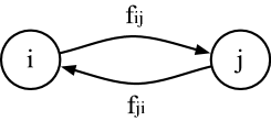
Figure 1: Schematic representation of mutual trust between two agents through the strengths of their links.

The idea behind the introduction of the forces $f_{ij}$ is loosely inspired by the potentiation/depotentiation of connections between neurons in neural networks, an effect known as the Hebb rule [31]. In our context, it can be seen as a kind of “memory” of previous encounters. However, it must be distinguished from the memory used in iterated games, in which players “remember” a certain number of previous moves and can thus conform their future strategy on the analysis of those past encounters [1]. Our interactions are strictly one-shot, i.e. players “forget” the results of previous rounds and cannot recognize previous partners and their possible playing patterns. However, a certain amount of past history is implicitly contained in the numbers $f_{ij}$ and this information may be used by an agent when it will come to decide whether or not an interaction should be dismissed (see below).
We also define a quantity $s_{i}$ called satisfaction of an agent $i$ which is the sum of all the weights of the links between $i$ and its neighbors $V_{i}$ divided by the total number of links $k_{i}$:

$$s_{i}=\frac{\sum_{j\in V_{i}}f_{ij}}{k_{i}}.$$

We clearly have $0\leq s_{i}\leq 1$. Note that the term satisfaction is sometimes used in game-theoretical work to mean the amount of utility gained by a given player. Instead, here satisfaction is related to the average willingness of a player to maintain the current relationships in the player’s neighborhood.

2.2 Initialization

The network is of constant size $N=1000$; this allows a simpler yet significant model of network dynamics in which social links may be broken and formed but agents do not disappear and new agents may not join the network. The initial graph is generated randomly with a mean degree $\bar{k}=10$ which is of the order of those actually found in many social networks such as collaboration, association, or friendship networks in which relations are generally rather long-lived and there is a cost to maintain a large number; see, for instance, [16, 12, 32, 33]. Players are distributed uniformly at random over the graph vertices with 50% cooperators. Forces of links between any pair of neighboring players are initialized at $0.5$.
We use a parameter $q$ which is akin to a “temperature” or noise level; $q$ is a real number in $[0,1]$ and it represents the frequency with which an agent wishes to dismiss a link with one of its neighbors. The higher $q$, the faster the link reorganization in the network. This parameter has been first introduced in [25] and it controls the speed at which topological changes occur in the network, i.e. the time scale of the strategy-topology co-evolution. It is an important consideration, as social networks may structurally evolve at widely different speeds, depending on the kind of interaction between agents. For example, e-mail networks change their structure at a faster pace than, say, scientific collaboration networks.

2.3 Strategy and Link Dynamics

Here we describe in detail how individual strategies, links, and link weights are updated. The node update sequence is chosen at random with replacement as in many previous works [34, 9, 26]. Once a given node $i$ of $G$ is chosen to be activated, it goes through the following steps:

• if the degree of agent $i$, $k_{i}=0$ then player $i$ is an isolated node. In this case a link with strength $0.5$ is created from $i$ to a player $j$ chosen uniformly at random among the other $N-1$ players in the network.

• otherwise,

  • either agent $i$ updates its strategy according to a local replicator dynamics rule with probability $1-q$ or, with probability $q$, agent $i$ may delete a link with a given neighbor $j$ and creates a new $0.5$ force link with another node $k$ ;

  • the forces between $i$ and its neighbors $V_{i}$ are updated

Let us now describe each step in more detail.

2.4 Strategy Evolution

We use a local version of replicator dynamics (RD) for regular graphs [9] but modified as described in [35] to take into account the fact that the number of neighbors in a degree-inhomogeneous network can be different for different agents. Indeed, it has been analytically shown that using straight accumulated payoff in degree-inhomogeneous networks leads to a loss of invariance with respect to affine transformations of the payoff matrix under RD [35]. The local dynamics of a player $i$ only depends on its own strategy and on the strategies of the $k_{i}$ players in its neighborhood $V_{i}\in G^{{}^{\prime}}$. Let us call $\pi_{ij}$ the payoff player $i$ receives when interacting with neighbor $j$. This payoff is defined as

$$\pi_{ij}=\sigma_{i}(t)\;M\;\sigma_{j}^{T}(t),$$

where $M$ is the payoff matrix of the game and $\sigma_{i}(t)$ and $\sigma_{j}(t)$ are the strategies played by $i$ and $j$ at time $t$. The quantity

$$\widehat{\Pi}_{i}(t)=\sum_{j\in V_{i}}\pi_{ij}(t)$$

is the weighted accumulated payoff defined in [35] collected by player $i$ at time step $t$. The rule according to which agents update their strategies is the conventional RD in which strategies that do better than the average increase their share in the population, while those that fare worse than average decrease. To update the strategy of player $i$, another player $j$ is drawn at random from the neighborhood $V_{i}$. It is assumed that the probability of switching strategy is a function $\phi$ of the payoff difference; $\phi$ is required to be monotonic increasing; here it has been taken linear [6]. Strategy $\sigma_{i}$ is replaced by $\sigma_{j}$ with probability

$$p_{i}=\phi(\widehat{\Pi}_{j}-\widehat{\Pi}_{i}),$$

where

$$\phi(\widehat{\Pi}_{j}-\widehat{\Pi}_{i})=\begin{cases}\dfrac{\widehat{\Pi}_{j}-\widehat{\Pi}_{i}}{\widehat{\Pi}_{j,\textrm{max}}-\widehat{\Pi}_{i,\textrm{min}}}&\textrm{if $\widehat{\Pi}_{j}-\widehat{\Pi}_{i}>0$}\\ \\ 0&\textrm{otherwise.}\end{cases}$$

In the last expression, $\widehat{\Pi}_{x,\textrm{max}}$ (resp. $\widehat{\Pi}_{x,\textrm{min}}$) is the maximum (resp. minimum) payoff a player $x$ can get (see ref. [35] for more details).

The major differences with standard RD is that two-person encounters between players are only possible among neighbors, instead of being drawn from the whole population, and the latter is of finite size in our case. Other commonly used strategy update rules include imitating the best in the neighborhood [7, 25], or replicating in proportion to the payoff  [9, 13].

2.5 Link Evolution

The active agent $i$, which has $k_{i}\neq 0$ neighbors will, with probability $q$, attempt to dismiss an interaction with one of its neighbors in the following way. In the description we focus on the outgoing links from $i$ in $G$, the incoming links play a subsidiary role. Player $i$ first looks at its satisfaction $s_{i}$. The higher $s_{i}$, the more satisfied the player, since a high satisfaction is a consequence of successful strategic interactions with the neighbors. Thus, the natural tendency is to try to dismiss a link when $s_{i}$ is low. This is simulated by drawing a uniform pseudo-random number $r\in[0,1]$ and breaking a link when $r\geq s_{i}$. Assuming that the decision is taken to cut a link, which one, among the possible $k_{i}$, should be chosen? Our solution is based on the strength of the relevant links. First a neighbor $j$ is chosen with probability proportional to $1-f_{ij}$, i.e. the stronger the link, the less likely it is that it will be selected. This intuitively corresponds to $i$’s observation that it is preferable to dismiss an interaction with a neighbor $j$ that has contributed little to $i$’s payoff over several rounds of play. However, dismissing a link is not free: $j$ may “object” to the decision. The intuitive idea is that, in real social situations, it is seldom possible to take unilateral decisions: often there is a cost associated, and we represent this hidden cost by a probability $1-(f_{ij}+f_{ji})/2$ with which $j$ may refuse to be cut away. In other words, the link is less likely to be deleted if $j$ appreciates $i$, i.e. when $f_{ji}$ is high.
Assuming that the $\vec{ij}$ and $\vec{ji}$ links are finally cut, how is a new interaction to be formed? The solution adopted here is inspired by the observation that, in social settings, links are usually created more easily between people who have a mutual acquaintance than those who do not. First, a neighbor $k$ is chosen in $V_{i}\setminus\{j\}$ with probability proportional to $f_{ik}$, thus favoring neighbors $i$ trusts. Next, $k$ in turn chooses player $l$ in his neighborhood $V_{k}$ using the same principle, i.e. with probability proportional to $f_{kl}$. If $i$ and $l$ are not connected, two links $\vec{il}$ and $\vec{li}$ are created, otherwise the process is repeated in $V_{l}$. Again, if the selected node, say $m$, is not connected to $i$, an interaction between $i$ and $m$ is established by creating two new links $\vec{im}$ and $\vec{mi}$. If this also fails, new links between $i$ and a randomly chosen node are created. In all cases the new links are initialized with a strength of $0.5$ in each direction. This rewiring process is schematically depicted in Fig. 2 for the case in which a link can be successfully established between players $i$ and $l$ thanks to their mutual acquaintance $k$.

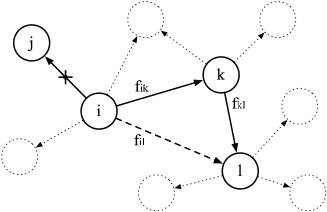
Figure 2: Illustration of the rewiring of link $\{ij\}$ to $\{il\}$. Agent $k$ is chosen to introduce player $l$ to $i$ (see text). Only outgoing links are shown for clarity.

At this point, we would like to stress several important differences with previous work in which links can be dismissed and rewired in a constant-size network in evolutionary games. First of all, in all these works the interaction graph is undirected with a single link between any pair of agents. In [25], only links between defectors are allowed to be cut unilaterally and the study is restricted to the Prisoner’s Dilemma. Instead, in our case, any interaction has a finite probability to be abandoned, even a profitable one between cooperators if it is recent, although links that are more stable, i.e. have high strengths, are less likely to be rewired. This smoother situation is made possible thanks to our bilateral view of a link. It also allows for a moderate amount of “noise”, which could reflect to some extent the uncertainties in the system. The present link rewiring process is also different from the one adopted in [27], where the Fermi function is used to decide whether to cut a link or not and also from their new version of it which has appeared in [28]. Finally, in [26] links are cut according to a threshold decision rule and are rewired randomly anywhere in the network.

2.6 Updating the Link Strengths

Once the chosen agents have gone through their strategy or link update steps, the strengths of the links are updated accordingly in the following way:

$$f_{ij}(t+1)=f_{ij}(t)+\frac{\pi_{ij}-\bar{\pi}_{ij}}{k_{i}(\pi_{max}-\pi_{min})},$$

where $\pi_{ij}$ is the payoff of $i$ when interacting with $j$, $\bar{\pi}_{ij}$ is the payoff earned by $i$ playing with $j$, if $j$ were to play his other strategy, and $\pi_{max}$ ($\pi_{min}$) is the maximal (minimal) possible payoff obtainable in a single interaction. If $f_{ij}(t+1)$ falls outside the $[0,1]$ interval then it is reset to $0$ if it is negative, and to $1$ if it is larger than $1$. This update is performed in both directions, i.e. both $f_{ij}$ and $f_{ji}$ are updated $\forall j\in V_{i}$ because both $i$ and $j$ get a payoff out of their encounter.

3 Numerical Simulations and Discussion

3.1 Simulation Parameters

We simulated the Hawks-Doves game with the dynamics described above exploring the game space by limiting our study to the variation of only two game parameters. We set $R=1$ and $P=0$ and the two parameters are $1\leq T\leq 2$ and $0\leq S\leq 1$. Setting $R=1$ and $P=0$ determines the range of $S$ (since $T>R>S>P$) and gives an upper bound of 2 for $T$, due to the $2R>T+S$ constraint, which ensures that mutual cooperation is preferred over an equal probability of unilateral cooperation and defection. Note however, that the only valid value pairs of $(T,S)$ are those that satisfy the latter constraint.

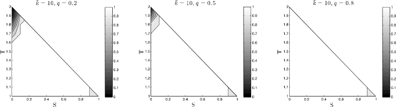
Figure 3: Average cooperation values for the Hawks-Doves game for three values of $q$ at steady-state. Results are the average of $50$ runs.

We simulated networks of size $N=1000$, randomly generated with an average degree $\bar{k}=10$ and randomly initialized with 50% cooperators and 50% defectors. In all cases, parameters $T$ and $S$ are varied between their two bounds in steps of 0.1. For each set of values, we carry out 50 runs of at most 10000 steps each, using a fresh graph realization in each run. Each step consists in the update of a full population. A run is stopped when all agents are using the same strategy, in order to be able to measure statistics for the population and for the structural parameters of the graphs. After an initial transient period, the system is considered to have reached a pseudo-equilibrium strategy state when the strategy of the agents (C or D) does not change over 150 further time steps, which means $15\times 10^{4}$ individual updates. It is worth mentioning that equilibrium is always attained well before the allowed $10000$ time steps, in most cases, less than $1^{\prime}000$ steps are enough. We speak of pseudo-equilibria or steady states and not of true evolutionary equilibria because there is no analog of equilibrium conditions in the dynamical systems sense.
To check whether scalability is an issue for the system, we have run several simulations with larger graphs namely, $N=3000$ and $N=10000$. The overall result is that, although the simulations take a little longer and transient times are also slightly longer, at quasi-equilibrium all the measures explored in the next sections follow the same trend and the dynamics give rise to comparable topologies and strategy relative abundance.

3.2 Emergence of Cooperation

Cooperation results in contour plot form are shown in Fig. 3. We remark that, as observed in other structured populations, cooperation is achieved in almost the whole configuration space. Thus, the added degree of freedom represented by the possibility of refusing a partner and choosing a new one does indeed help to find player’s arrangements that help cooperation. When considering the dependence on the parameter $q$, one sees in Fig. 3 that the higher $q$, the higher the cooperation level, although the differences are small, since full cooperation prevails already at $q=0.2$. This is a somewhat expected result, since being able to break ties more often clearly gives cooperators more possibilities for finding and keeping fellow cooperators to interact with. The results reported in the figures are for populations starting with $50\%$ cooperators randomly distributed. We have also tried other proportions with less cooperators, starting at $30\%$. The results, not reported here for reasons of space, are very similar, the only difference being that it takes more simulation time to reach the final quasi-stable state. Finally, one could ask whether cooperation would still spread starting with very few cooperators. Numerical simulations show that cooperation could indeed prevail even starting from as low as $1\%$ cooperators, except on the far left border of the configuration space where cooperation is severely disadvantaged.
Compared with the level of cooperation observed in simulations in static networks, we can say that results are consistently better for co-evolving networks. For all values of $q$ (Fig. 3) there is significantly more cooperation than what was found in model and real social networks [19] where the same local replicator dynamics was used but with the constraints imposed by the invariant network structure. A comparable high cooperation level has only been found in static scale-free networks [14, 36] which are not as realistic as a social network structures.
The above considerations are all the more interesting when one observes that the standard RD result is that the only asymptotically stable state for the game is a polymorphic population in which there is a fraction $\alpha$ of doves and a fraction $1-\alpha$ of hawks, with $\alpha$ depending on the actual numerical payoff matrix values. To see the positive influence of making and breaking ties we can compare our results with what is prescribed by the standard RD solution. Referring to the payoff table 1, let’s assume that the column player plays C with probability $\alpha$ and D with probability $1-\alpha$. In this case, the expected payoffs of the row player are:

$$E_{r}[C]=\alpha R+(1-\alpha)S$$

and

$$E_{r}[D]=\alpha T+(1-\alpha)P$$

The row player is indifferent to the choice of $\alpha$ when $E_{r}[C]=E_{r}[D]$. Solving for $\alpha$ gives:

$$\alpha=\frac{P-S}{R-S-T+P}.$$ (1)

Since the game is symmetric, the result for the column player is the same and $(\alpha C,(1-\alpha)D)$ is a NE in mixed strategies. We have numerically solved the equation for all the sampled points in the game’s parameter space. Let us now use the following payoff values in order to bring them within the explored game space (remember that NEs are invariant w.r.t. such an affine transformation):

	C	D
C	($1,1$)	($2/3,4/3$)
D	($4/3,2/3$)	($0,0$)

Substituting in equation 1 gives $\alpha=2/3$, i.e. the dynamically stable polymorphic population should be composed by about $2/3$ cooperators and $1/3$ defectors. Now, if one looks at Fig. 3 at the points where $S=2/3$ and $T=4/3$, one can see that the point, and the region around it, is one of full cooperation instead. Even within the limits of the approximations caused by the finite population size and the local dynamics, the non-homogeneous graph structure and an increased level of tie rewiring has allowed cooperation to be greatly enhanced with respect to the theoretical predictions of standard RD.

3.3 Evolution of Agents’ Satisfaction

According to the model, unsatisfied agents are more likely to try to cut links in an attempt to improve their satisfaction level, which could be simply described as an average value of the strengths of their links with neighbors. Satisfaction should thus tend to increase during evolution. In effect, this is what happens, as can be seen in Fig. 4. The figure refers to a particular run that ends in all agents cooperating, but it is absolutely typical.

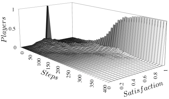
Figure 4: Fraction of agents having a given satisfaction level as a function of evolution time.

One can remark the “spike” at time $0$. This is clearly due to the fact that all links are initialized with a weight of $0.5$. As the simulation advances, the satisfaction increases steadily and for the case of the figure, in which all agents cooperate at the end, it reaches its maximum value of $1$ for almost all players.

3.4 Stability of Cooperation

Evolutionary game theory provides a dynamical view of conflicting decision-making in populations. Therefore, it is important to assess the stability of the equilibrium configurations. This is even more important in the case of numerical simulation where the steady-state finite population configurations are not really equilibria in the mathematical sense. In other words, one has to be reasonably confident that the steady-states are not easily destabilized by perturbations. To this end, we have performed a numerical study of the robustness of final cooperators’ configurations by introducing a variable amount of random noise into the system. A strategy is said to be evolutionarily stable when it cannot be invaded by a small amount of players using another strategy [6]. We have chosen to switch the strategy of an increasing number of highly connected cooperators to defection, and to observe whether the perturbation propagates in the population, leading to total defection, or if it stays localized and disappears after a transient time.

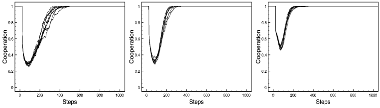
Figure 5: Cooperation percentage as a function of simulated time when the strategy of the $30\%$ most connected nodes is switched from cooperation to defection. $T=1.6$, $S=0.4$ and, from left to right, $q=0.2,0.5,0.8$.

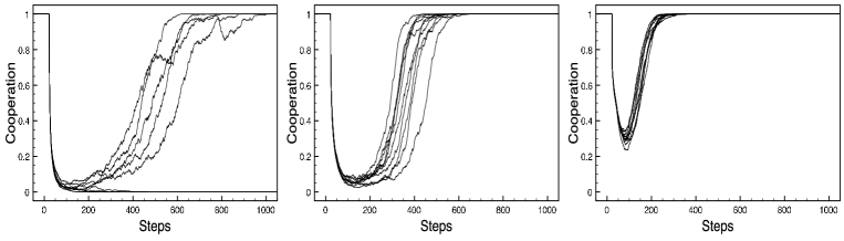
Figure 6: Cooperation percentage when the strategy of the $30\%$ most connected nodes is switched from cooperation to defection. $T=1.9$, $S=0.1$ and, from left to right, $q=0.2,0.5,0.8$.

Figs. 5 and 6 show how the system recovers when the most highly connected $30$% of the cooperators are suddenly and simultaneously switched to defection. In Fig. 5 the value chosen in the game’s configuration space is $T=1.6$ and $S=0.4$. This point lies approximately on the diagonal in Fig. 3 and corresponds to an all-cooperate situation. As one can see, after the perturbation is applied, there is a sizable loss of cooperation but, after a while, the system recovers full cooperation in all cases (only $10$ curves are shown in each figure for clarity, but the phenomenon is qualitatively identical in all the $50$ independent runs tried). From left to right, three values of $q=0.2,0.5,0.8$ are used. It is seen that, as the rewiring frequency $q$ increases, recovering from the perturbation becomes easier as defection has less time to spread around before cooperators are able to dismiss links toward defectors. Switching the strategy of the $30$ % most connected nodes is rather extreme since they include most cooperator clusters but, nonetheless, cooperation is rather stable in the whole cooperating region. In Fig. 6 we have done the same this time with $T=1.9$ and $S=0,1$. This point is in a frontier region in which defection may often prevail, at least for low $q$ (see Fig. 3) and thus it represents one of the hardest cases for cooperation to remain stable. Nevertheless, except in the leftmost case ($q=0.2$) where half of the runs permanently switch to all-defect, in all the other cases the population is seen to recover after cooperation has fallen down to less than $10\%$. Note that the opposite case is also possible in this region that is, in a full defect situation, switching of $30\%$ highly connected defectors to cooperation can lead the system to one of full cooperation. In conclusion, the above numerical experiments have empirically shown that cooperation is extremely stable after cooperator networks have emerged. Although we are using here an artificial society of agents, this can hopefully be seen as an encouraging result for cooperation in real societies.

3.5 Structure of the Emerging Networks

In this section we present a statistical analysis of the global and local properties of the networks that emerge when the pseudo-equilibrium states of the dynamics are attained. Note that in the following sections the graph we refer to is the unoriented, unweighted one that we called $G^{{}^{\prime}}$ in Sect. 2.1. In other words, for the structural properties of interest, we only take into account the fact that two agents interact and not the weights of their directed interactions.

3.5.1 Small-World Nature

Small-world networks are characterized by a small mean path length and by a high clustering coefficient [11]. Our graphs start random, and thus have short path lengths by construction since their mean path length $\bar{l}=O(logN)$ scales logarithmically with the number of vertices $N$ [12]. It is interesting to notice that they maintain short diameters at equilibrium too, after rewiring has taken place. We took the average $\bar{L}=\sum_{k=1}^{660}\bar{l}$ of the mean path length of $660$ evolved graphs, which represent ten graphs for each $T,S$ pair. This average is 3.18, which is of the order of $log(1000)$, while its initial random graph average value is $3.25$. This fact, together with the remarkable increase of the clustering coefficients with respect to the random graph (see below), shows that the evolved networks have the small-world property. Of course, this behavior was expected, since the rewiring mechanism favors close partners in the network and thus tends to increase the clustering and to shorten the distances.

3.5.2 Average Degree

In contrast to other models [25, 27], the mean degree $\bar{k}$ can vary during the course of the simulation. We found that $\bar{k}$ increases only slightly and tends to stabilize around $\bar{k}=11$. This is in qualitative agreement with observations made on real dynamical social networks [20, 37, 38] with the only difference that the network does not grow in our model.

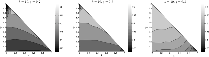
Figure 7: Average values of the clustering coefficient over $50$ runs for three values of $q$.

3.5.3 Clustering Coefficients

The clustering coefficient $\cal C$ of a graph has been defined in the Introduction section. Random graphs are locally homogeneous in the average and for them $\cal C$ is simply equal to the probability of having an edge between any pair of nodes independently. In contrast, real networks have local structures and thus higher values of $\cal C$. Fig. 7 gives the average clustering coefficient $\bar{\cal C}=\frac{1}{50}\sum_{i=1}^{50}{\cal C}$ for each sampled point in the Hawks-Doves configuration space, where $50$ is the number of network realizations used for each simulation. The networks self-organize through dismissal of partners and choice of new ones and they acquire local structure, since the clustering coefficients are higher than that of a random graph with the same number of edges and nodes, which is $\bar{k}/N=10/1000=0.01$. The clustering tends to increase with $q$ (i.e. from left to right in Fig. 7). It is clear that the increase in clustering and the formation of cliques is due to the fact that, when dismissing an unprofitable relation and searching for a new one, individuals that are relationally at a short distance are statistically favored. But this has a close correspondence in the way in which new acquaintances are made in society: they are not random, rather people often get to interact with each other through common acquaintances, or “friends of friends” and so on.

3.5.4 Degree Distributions

The degree distribution function (DDF) $p(k)$ of a graph represents the probability that a randomly chosen node has degree $k$. Random graphs are characterized by DDF of Poissonian form $p(k)={\bar{k}}^{k}e^{-\bar{k}}/k!$, while social and technological real networks often show long tails to the right, i.e. there are nodes that have an unusually large number of neighbors [12]. In some extreme cases the DDF has a power-law form $p(k)\propto k^{-\gamma}$; the tail is particularly extended and there is no characteristic degree. The cumulative degree distribution function (CDDF) is just the probability that the degree is greater than or equal to $k$ and has the advantage of being less noisy for high degrees. Fig. 8 shows the CDDFs for the Hawks-Doves for three values of $T$, $S=0.2$, and $q=0.5$ with a logarithmic scale on the y-axis. A Poisson and an exponential distribution are also included for comparison. The Poisson curve actually represents the initial degree distribution of the (random) population graph. The distributions at equilibrium are far from the Poissonian that would apply if the networks would remain essentially random. However, they are also far from the power-law type, which would appear as a straight line in the log-log plot of Fig 9.

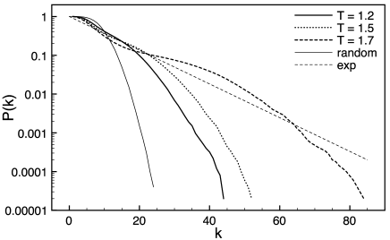
Figure 8: Empirical cumulative degree distribution functions for three different values of the temptation $T$. A Poissonian and an exponential distribution are also plotted for comparison. Distributions are discrete, the continuous lines are only a guide for the eye. Lin-log scales.

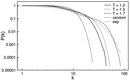
Figure 9: Empirical cumulative degree distribution functions for three different values of the parameter $T$. Log-log scales.

Although a reasonable fit with a single law appears to be difficult, these empirical distributions are closer to exponentials, in particular the curve for $T=1.7$, for which such a fit has been drawn. It can be observed that the distribution is broader the higher $T$ (The higher $T$, the more agents gain by defecting). In fact, although cooperation is attained nearly everywhere in the game’s configuration space, higher values of the temptation $T$ mean that agents have to rewire their links more extensively, which results in a higher number of neighbors for some players, and thus it leads to a longer tail in the CDDF.

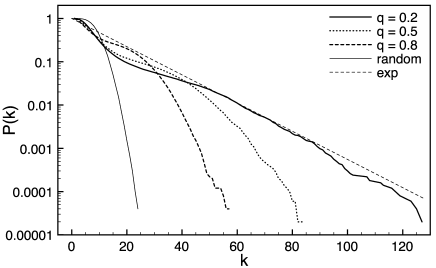
Figure 10: Empirical cumulative degree distribution functions for three different values of the temptation $q$. Lin-log scales.

The influence of the $q$ parameter on the shape of the degree distribution functions is shown in Fig. 10 where average curves for three values of $q$, $T=1.7$, and $S=0.2$, are reported. For high $q$, the cooperating steady-state is reached faster, which gives the network less time to rearrange its links. For lower values of $q$ the distributions become broader, despite the fact that rewiring occurs less often, because cooperation in this region is harder to attain and more simulation time is needed. In conclusion, emerging network structures at steady states have DDFs that are similar to those found in actual social networks [12, 15, 16, 17, 33], with tails that are fatter the higher the temptation $T$ and the lower $q$. Topologies closer to scale-free would probably be obtained if the model allowed for growth, since preferential attachment is already present to some extent due to the nature of the rewiring process [39].

3.5.5 Degree Correlations

Besides the degree distribution function of a network, it is also sometimes useful to investigate the empirical joint degree-degree distribution of neighboring vertices. However, it is difficult to obtain reliable statistics because the data set is usually too small (if a network has $L$ edges, with $L\ll N^{2}$ where $N$ is the number of vertices for the usually relatively sparse networks we deal with, one then has only $L$ pairs of data to work with). Approximate statistics can readily be obtained by using the average degree of the nearest neighbors of a vertex $i$ as a function of the degree of this vertex, $\bar{k}_{V_{i}}(k_{i})$ [40].

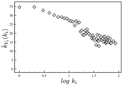
Figure 11: Average degree of the direct neighbors of a vertex Vs. the vertex degree. The relation is disassortative. Log-lin scales.

From Fig. 11 one can see that the correlation is slightly negative, or disassortative. This is at odds with what is reported about real social networks, in which usually this correlation is positive instead, i.e. high-degree nodes tend to connect to high-degree nodes and vice-versa [12]. However, real social networks establish and grow because of common interests, collaboration work, friendship and so on. Here this is not the case, since the network is not a growing one, and the game played by the agents is antagonistic and causes segregation of highly connected cooperators into clusters in which they are surrounded by less highly connected fellows. This will be seen more pictorially in the following section.

3.6 Cooperator Clusters

From the results of the previous sections, it appears that a much higher amount of cooperation than what is predicted by the standard theory for mixing populations can be reached when ties can be broken and rewired. We have seen that this dynamics causes the graph to acquire local structure, and thus to loose its initial randomness. In other words, the network self-organizes in order to allow players to cooperate as much as possible. At the microscopic, i.e. agent level, this happens through the formation of clusters of players using the same strategy. Fig. 12 shows one typical cooperator cluster.

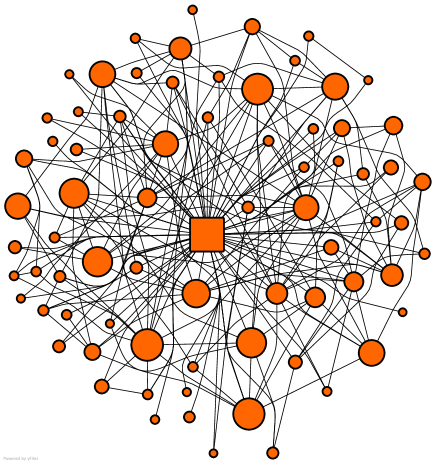
Figure 12: A typical cooperator cluster. Links to the rest of the network have been suppressed for clarity. The size of a node is proportional to its connectivity in the whole graph. The most connected central cooperator is shown as a square.

In the figure one can clearly see that the central cooperator is a highly connected node and there are many links also between the other neighbors. Such tightly packed structures have emerged to protect cooperators from defectors that, at earlier times, were trying to link to cooperators to exploit them. These observations help understand why the degree distributions are long-tailed (see previous section), and also the higher values of the clustering coefficient.
Further studies of the emerging networks would imply investigating the communities and the way in which strategies are distributed in them. There are many ways to reveal the modular structure of networks [41] but we leave this study for further work.

4 Conclusions

In this paper we have introduced a new dynamical population structure for agents playing a series of two-person Hawks and Doves game. The most novel feature of the model is the adoption of a variable strength of the bi-directional social ties between pairs of players. These strengths change dynamically and independently as a function of the relative satisfaction of the two end points when playing with their immediate neighbors in the network. A player may wish to break a tie to a neighbor and the probability of cutting the link is higher the weaker the directed link strength is. The ensemble of weighted links implicitly represents a kind of memory of past encounters although, technically speaking, the game is not iterated. While in previous work the rewiring parameters where ad hoc, unspecified probabilities, we have made an effort to relate them to the agent’s propensity to gauge the perceived quality of a relationship during time.
The model takes into account recent knowledge coming from the analysis of the structure and of the evolution of social networks and, as such, should be a better approximation of real social conflicting situations than static graphs such as regular grids. In particular, new links are not created at random but rather taking into account the “trust” a player may have on her relationally close social environment as reflected by the current strengths of its links. This, of course, is at the origin of the de-randomization and self-organization of the network, with the formation of stable clusters of cooperators. The main result concerning the nature of the pseudo-equilibrium states of the dynamics is that cooperation is greatly enhanced in such a dynamical artificial society and, furthermore, it is quite robust with respect to large strategy perturbations. Although our model is but a simplified and incomplete representation of social reality, this is encouraging, as the Hawks-Doves game is a paradigm for a number of social and political situations in which aggressivity plays an important role. The standard result is that bold behavior does not disappear at evolutionary equilibrium. However, we have seen here that a certain amount of plasticity of the networked society allows for full cooperation to be consistently attained. Although the model is an extremely abstract one, it shows that there is place for peaceful resolution of conflict. In future work we would like to investigate other stochastic strategy evolution models based on more refined forms of learning than simple imitation and study the global modular structure of the equilibrium networks.

Acknowledgements. This work is funded by the Swiss National Science Foundation under grant number 200020-119719. We gratefully acknowledge this financial support.

References

- [1] F. Vega-Redondo, Economics and the Theory of Games, Cambridge University Press, Cambridge, UK, 2003.
- [2] R. Axelrod, The Evolution of Cooperation, Basic Books, Inc., New-York, 1984.
- [3] K. Lindgren, M. G. Nordahl, Evolutionary dynamics of spatial games, Physica D 75 (1994) 292–309.
- [4] W. Poundstone, The Prisoner’s Dilemma, Doubleday, New York, 1992.
- [5] J. Maynard Smith, Evolution and the Theory of Games, Cambridge University Press, 1982.
- [6] J. Hofbauer, K. Sigmund, Evolutionary Games and Population Dynamics, Cambridge University Press, Cambridge, UK, 1998.
- [7] M. A. Nowak, R. M. May, Evolutionary games and spatial chaos, Nature 359 (1992) 826–829.
- [8] T. Killingback, M. Doebeli, Spatial evolutionary game theory: hawks and doves revisited, Proceedings of the Royal Society of London B 263 (1996) 1135–1144.
- [9] C. Hauert, M. Doebeli, Spatial structure often inhibits the evolution of cooperation in the snowdrift game, Nature 428 (2004) 643–646.
- [10] G. Szabó, G. Fáth, Evolutionary games on graphs, Physics Reports 446 (2007) 97–216.
- [11] D. J. Watts, S. H. Strogatz, Collective dynamics of ’small-world’ networks, Nature 393 (1998) 440–442.
- [12] M. E. J. Newman, The structure and function of complex networks, SIAM Review 45 (2003) 167–256.
- [13] M. Tomassini, L. Luthi, M. Giacobini, Hawks and doves on small-world networks, Phys. Rev. E 73 (2006) 016132.
- [14] F. C. Santos, J. M. Pacheco, Scale-free networks provide a unifying framework for the emergence of cooperation, Phys. Rev. Lett. 95 (2005) 098104.
- [15] L. A. N. Amaral, A. Scala, M. Barthélemy, H. E. Stanley, Classes of small-world networks, Proc. Natl. Acad. Sci. USA 97 (2000) 11149–11152.
- [16] M. E. J. Newman, Scientific collaboration networks. I. network construction and fundamental results, Phys. Rev E 64 (2001) 016131.
- [17] P. Jordano, J. Bascompte, J. Olesen, Invariant properties in coevolutionary networks of plant-animal interactions, Ecology Letters 6 (2003) 69–81.
- [18] F. Liljeros, C. R. Edling, L. A. N. Amaral, H. E. Stanley, Y. Aberg, The web of human sexual contacts, Nature 411 (2001) 907–908.
- [19] L. Luthi, E. Pestelacci, M. Tomassini, Cooperation and community structure in social networks, Physica A 387 (2008) 955–966.
- [20] G. Kossinets, D. J. Watts, Empirical analysis of an evolving social network, Science 311 (2006) 88–90.
- [21] J. Batali, P. Kitcher, Evolution of altruism in optional compulsory games, J. Theor. Biol. 175 (1995) 161–171.
- [22] T. N. Sherratt, G. Roberts, The evolution of generosity and choosiness in cooperative exchanges, J. Theor. Biol. 193 (1998) 167–177.
- [23] B. Skyrms, R. Pemantle, A dynamic model for social network formation, Proc. Natl. Acad. Sci. USA 97 (2000) 9340–9346.
- [24] V. M. Eguíluz, M. G. Zimmermann, C. J. Cela-Conde, M. S. Miguel, Cooperation and the emergence of role differentiation in the dynamics of social networks, American J. of Sociology 110 (4) (2005) 977–1008.
- [25] M. G. Zimmermann, V. M. Eguíluz, Cooperation, social networks, and the emergence of leadership in a prisoner’s dilemma with adaptive local interactions, Phys. Rev. E 72 (2005) 056118.
- [26] L. Luthi, M. Giacobini, M. Tomassini, A minimal information prisoner’s dilemma on evolving networks, in: L. M. Rocha (Ed.), Artificial Life X, The MIT Press, Cambridge, Massachusetts, 2006, pp. 438–444.
- [27] F. C. Santos, J. M. Pacheco, T. Lenaerts, Cooperation prevails when individuals adjust their social ties, PLOS Comp. Biol. 2 (2006) 1284–1291.
- [28] S. V. Segbroeck, F. C. Santos, A. Nowé, J. M. Pacheco, T. Lenaerts, The evolution of prompt reaction to adverse ties, BMC Evolutionary Biology 8 (2008) 287.
- [29] E. Pestelacci, M. Tomassini, Hawks and doves in an artificial dynamically structured society, in: Artificial Life XI, 2008.
- [30] E. Pestelacci, M. Tomassini, L. Luthi, Evolution of cooperation and coordination in a dynamically networked society, J. of Biological Theory 3 (2) (2008) 139–153.
- [31] D. O. Hebb, The Organization of Behavior, Wiley, New York, 1949.
- [32] J. Moody, The structure of a social science collaboration network: disciplinary cohesion from 1963 to 1999, American Sociological Review 69 (2004) 213–238.
- [33] M. Tomassini, L. Luthi, M. Giacobini, W. B. Langdon, The structure of the genetic programming collaboration network, Genetic Programming and Evolvable Machines 8 (1) (2007) 97–103.
- [34] B. A. Huberman, N. S. Glance, Evolutionary games and computer simulations, Proc. Natl. Acad. Sci. USA 90 (1993) 7716–7718.
- [35] L. Luthi, M. Tomassini, E. Pestelacci, Evolutionary games on networks and payoff invariance under replicator dynamics, BiosystemsTo appear.
- [36] F. C. Santos, J. M. Pacheco, T. Lenaerts, Evolutionary dynamics of social dilemmas in structured heterogeneous populations, Proc. Natl. Acad. Sci. USA 103 (2006) 3490–3494.
- [37] A.-L. Barabási, H. Jeong, Z. Néda, E. Ravasz, A. Schubert, T. Vicsek, Evolution of the social network of scientific collaborations, Physica A 311 (2002) 590–614.
- [38] M. Tomassini, L. Luthi, Empirical analysis of the evolution of a scientific collaboration network, Physica A 385 (2007) 750–764.
- [39] J. Poncela, J. G.-G. nes, L. M. Floria, A. Sánchez, Y. Moreno, Complex cooperative networks from evolutionary preferential attachment, Plos ONE 3 (2008) e2449.
- [40] R. Pastor-Satorras, A. Vázquez, A. Vespignani, Dynamical and correlation properties of the Internet, Phys. Rev. Lett. 87 (2001) 258701.
- [41] L. Danon, A. Díaz-Guilera, J. Duch, A. Arenas, Comparing community structure identification, J. Stat. Mech. (2005) P09008.