New identified (³H)4d-(³H)4f transitions of Fe ii from UVES spectra of HR 6000 and 46 Aql

Abstract

Aims. The analysis of the high-resolution UVES spectra of the CP stars HR 6000 and 46 Aql has revealed the presence of an impressive number of unidentified lines, in particular in the 5000-5400 Å region. Because numerous 4d-4f transitions of Fe ii lie in this spectral range, and because both stars are iron overabundant, we investigated whether the unidentified lines can be due to Fe ii.

Methods. ATLAS12 model atmospheres with parameters [13450K,4.3] and [12560K,3.8] were computed for the individual abundances of HR 6000 and 46 Aql, respectively, in order to use the stars as spectroscopic sources to identify Fe ii lines and to determine Fe ii gf-values. After having identified several unknown lines in the stellar spectra as due to (³H)4d$-$(³H)4f transitions of Fe ii, we derived stellar $\log\,gf$’s for them by comparing observed and computed profiles. The energies of the upper levels were assigned on the basis of both laboratory iron spectra and predicted energy levels.

Results. We fixed 21 new levels of Fe ii with energies between 122910.9 cm^-1 and 123441.1 cm^-1. They allowed us to add 1700 new lines to the Fe ii line list in the range 810 $-$ 15011 Å.

1 Introduction

The analysis of the UVES spectrum of the chemically peculiar star HR 6000 performed by Castelli & Hubrig (2007) has shown the presence of a huge number of unidentified lines in the whole observed range from 3050 Å to 9460 Å. Most impressive regions were those at 4404-4411 Å  and 5000-5400 Å. An attempt to identify unknown lines in the 5130-5136 Å interval using the available lists of predicted Fe ii lines (version 2003) was very laborious and not very successful.

An analysis of the list of the unidentified lines and of the plot of the observed and computed spectra available at the Castelli web-site has led S. Johansson to identify about half of them as transitions between high excitation levels of Fe ii. The identifications were made using unpublished line lists he obtained from laboratory spectra. Johansson (2009) was able to fix a group of 13 lines concentrated in the 4404-4411 Å interval as belonging to the multiplet 4s(⁷S)4d ⁸D $-$ 4s(⁷S)4f ⁸F. The upper terms have energies between 132145 cm^-1 and 132158 cm^-1, therefore well above the Fe ii ionization limit of 130563 cm^-1. Another example of new identifications can be found in Castelli, Johansson & Hubrig (2008) where some unknown lines in the 5175-5180 Å interval of HR 6000 were identified as due to (³H)4d $-$ (³H)4f transitions of Fe ii. In this case the energy of the upper levels is of the order of 123000 cm^-1, therefore just below the ionization limit.

Laboratory spectroscopic sources show lines in emission and must populate upper levels to produce a spectrum. Most stars are observed in absorption so that their line strengths are determined by the lower level populations; the spectra are stronger. HR 6000 and 46 Aql are bright and can be observed at high resolution and high signal-to-noise ratio. They have low projected rotation velocity, 1.5 km s^-1 for HR 6000 and 1.0 km s^-1 for 46 Aql. Thus blending is minimal and wavelengths and line strengths can be well determined by fitting the spectrum.

It is likely that most of the unidentified lines in these stars are Fe ii. Some could be due to other overabundant elements, in particular P ii, Mn ii and Xe ii. However, as far as Mn ii is concerned, the unidentified lines are either weaker or do not appear at all in the HgMn star HD 175640 which is iron weak ([Fe/H]= $-$0.25) and manganese overabundant ([Mn/H]= +2.4) (Castelli & Hubrig 2004; Castelli et al. 2008). It is also improbable that so large number of unidentified lines, mostly concentrated in the 5000-6000 Å region, are not also due to Fe ii. Since these lines are present at subsolar iron abundance they must be present in all Population I late B-type stars, or in any object with strong Fe ii lines, but they are normally smeared out by rotation and difficult to see.

Because every new level accounts for hundreds of new lines throughout the spectrum from the UV through the IR, we extended to a larger range the work already made for the 5175-5181 Å interval with the aim to increase the number of the classified Fe ii levels. We used both identifications based on laboratory spectra and derived from predicted energy levels. Furthermore, because numerous high-excitation lines due to the 3d⁶(⁵D)4d $-$ 3d⁶(⁵D)4f transitions lie in the 5000$-$5400 Å interval, we examined the computed $\log\,gf$’s that are used for the synthetic spectra computations. We compared them with experimental (Johansson, 2002) and stellar values, which we derived from both HR 6000 and 46 Aql. We used two stars in order to check the consistency and estimate the reliability of the stellar oscillator strengths. Then, we derived stellar $\log$ gf’s for the new identified (³H)4d $-$ (³H)4f lines. Finally, we show an example of synthetic spectrum computed both with old and new line lists.

In order to use HR 6000 and 46 Aql as spectroscopic sources to identify Fe ii lines, to determine Fe ii $\log\,gf$’s, and to compute synthetic spectra we fixed at first model atmospheres and abundances for each star. Special care was devoted to derive the iron abundance.

2 The stars HR 6000 and 46 Aql

Both HR 6000 (HD 144667) and 46 Aql (HD 186122) are B-type CP stars. HR 6000 was extensively studied by Castelli & Hubrig (2007) in the 3050 $-$ 9460 Å region, 46 Aql by Sadakane et al. (2001) in the 5100 $-$ 6400 Å interval. Because model atmospheres are needed for the determination of stellar $\log\,gf$’s, we revised the model atmosphere and the abundances of HR 6000 and determined the model atmosphere and the abundances for 46 Aql on the basis of our observations.

2.1 Observations

The observations of HR 6000 are described in Castelli & Hubrig (2007). Those for 46 Aql were obtained in the framework of the same observational program (ESO prg. 076.D-0169(A)). They are of the same quality and were reduced with the same procedures used for HR 6000.

In this paper we revised our previous analysis of HR 6000 (Castelli & Hubrig 2007) because a further investigation has indicated that Balmer profiles that were used by us to fix the model parameters are too affected in the UVES spectra by imperfections related to the echelle orders. As we show in Appendix A, the spectral distorsions for H_δ, H_γ, and, to a less extent, for H_β are so significant that it is not possible to draw a reliable continuum over the observed profiles. Only H$\alpha$ does not show manifest problems so that it could be used for the analysis with some confidence.

2.2 Model paramaters and abundances

In Castelli & Hubrig (2007) the model parameters of HR 6000 ($T_{\rm eff}$=12850 K, $\log\,g$=4.10, $\xi$=0.0 km s^-1) were derived from Balmer profiles and from Fe i and Fe ii ionization equilibrium. In this paper the model parameters for both HR 6000 and 46 Aql were obtained from the Strömgren photometry, from the requirement of no correletion of Fe ii abundances derived from high and low excitation lines, and from the requirement of Fe i $-$ Fe ii ionization equilibrium. This kind of determination has led to a revision of the model parameters for HR 6000.

Table 1: Observed and dereddened Strömgren indices for HR 6000 and 46 Aql.

Star	b$-$y	m	c	$\beta$	E(b-y)	(b-y)0	m0	c0	$T_{\rm eff}$(K)	$\log\,g$
HR 6000	$-$0.030	0.116	0.521	2.750	0.031	$-$0.061	0.126	0.506	13799$\pm$150	4.27$\pm$0.05
	$\pm$0.003	$\pm$0.003	$\pm$0.003
46 Aql	$-$0.019	0.094	0.641	2.729	0.035	$-$0.054	0.105	0.634	12763$\pm$150	3.75$\pm$0.05
	$\pm$0.002	$\pm$0.002	$\pm$0.002

The parameters of the two stars obtained from the Strömgren photometry are given in Table 1. They were derived with the method described in Castelli & Hubrig (2007), where the reddening for HR 6000 is also dicussed. The observed indices were taken from the Hauck& Mermilliod (1998) Catalogue. ATLAS9 models with parameters [13800K,4.3] for HR 6000 and [12750K,3.8] for 46 Aql were computed for solar abundances and zero microturbulent velocity. The iron abundance was derived from the equivalent widths of a selected sample of high-excitation Fe ii lines having experimental $\log\,gf$’s (Johansson, 2002). They are due to (⁵D)4d $-$ (⁵D)4f transitions and are listed in Table 2. The equivalent widths of these lines, as well as of the other lines discussed in this paper, were measured integrating the residual fluxes over the profiles. Abundances were obtained with a Linux version (Castelli 2005) of the WIDTH code (Kurucz 1993). We note that there are no measured equivalent widths for the line at 5100.734 Å because it is part of a strong blend formed by four Fe ii lines. The line was included in Table 2 in order to show the whole set of (⁵D)4d $-$ (⁵D)4f transitions having experimental $\log\,gf$’s. The lines from Table 2 are particularly well suited to provide the iron abundance because they are rather insensitive to the model parameters. In fact, for differences in $T_{\rm eff}$ of 500 K, they give abundance differences less than 0.05 dex. For difference in $\log\,g$ of 0.2 dex they give abundance differences of the order of 0.01 dex. For example, for HR 6000, the Fe ii abundance from ATLAS9 models computed for $\log\,g$=4.3 and $T_{\rm eff}$= 13300 K, 13800 K, and 14300 K is $-$3.66 dex , $-$3.65 dex (Table 2), and $-$3.61 dex, respectively. For models computed for $T_{\rm eff}$=13800 K and $\log\,g$=4.1, 4.3, and 4.5 the iron abundance is $-$3.65 dex, $-$3.65 dex (Table 2), and $-$3.64 dex. Similar results can be obtained for 46 Aql.

Table 2: Iron abundance from a selected sample of high excitation (4d-4f) Fe ii lines with experimental $\log$ gf’s and ATLAS9 models.

$\lambda$($\AA$)	$\log$ gf	$\chi_{low}$(cm-1)	$\chi_{up}$(cm-1)	Config.	W(mÅ)	$\log$$\epsilon$(W)	W(mÅ)	$\log$$\epsilon$(W)
	exp				HR 6000 [13800,4.3]		46 Aql [12750,3.8]
4883.292	$-$0.521	82853.66	103325.93	(5D)4d e6F11/2$-$ (5D)4f 3[5]11/2	14.2	$-$3.87	11.3	$-$4.10
4913.295	0.016	82978.67	103325.93	(5D)4d e6F9/2$-$ (5D)4f 3[5]11/2	36.3	$-$3.67	31.1	$-$3.91
5001.953	0.933	82853.66	102840.27	(5D)4d e6F11/2$-$ (5D)4f 4[6]13/2	76.0	$-$3.61	66.1	$-$3.86
5100.734	0.671	83726.37	103325.93	(5D)4d 6D9/2$-$ (5D)4f 3[5]11/2	$--$	$--$	$--$	$--$
5227.483	0.831	84296.83	103421.16	(5D)4d e6G11/2$-$ (5D)4f 3[6]13/2	66.8	$-$3.58	58.0	$-$3.83
5253.647	$-$0.191	84296.83	103325.93	(5D)4d e6G11/2$-$ (5D)4f 3[5]11/2	30.6	$-$3.51	23.5	$-$3.83
5260.254	1.090	84035.12	103040.32	(5D)4d e6G13/2$-$ (5D)4f 4[7]15/2	77.9	$-$3.59	66.9	$-$3.84
5316.214	0.418	84035.12	102840.27	(5D)4d e6G13/2$-$ (5D)4f 4[6]13/2	48.7	$-$3.61	39.7	$-$3.94
5339.592	0.568	84296.83	103019.64	(5D)4d e6G11/2$-$ (5D)4f 4[7]13/2	48.2	$-$3.74	42.8	$-$3.97
5387.063	0.593	84863.33	103421.16	(5D)4d e4G11/2$-$ (5D)4f 3[6]13/2	47.7	$-$3.75	41.3	$-$4.00
5414.852	$-$0.258	84863.33	103325.93	(5D)4d e4G11/2$-$ (5D)4f 3[5]11/2	25.0	$-$3.57	19.1	$-$3.87
5506.199	0.923	84863.33	103019.64	(5D)4d e4G11/2$-$ (5D)4f 4[7]13/2	73.8	$-$3.65	54.2	$-$3.94
5510.783	0.043	85184.73	103325.93	(5D)4d e4G9/2$-$ (5D)4f 3[5]11/2	32.5	$-$3.61	26.3	$-$3.89
Average abundances						$-$3.65$\pm$0.09		$-$3.92$\pm$0.08

Once the iron abundance was fixed, we checked the model parameters inquiring whether the adopted model gives the same abundance also from Fe i lines and from a large sample of Fe ii lines which includes also low-excitation transitions. To this purpose, we measured the equivalent widths of the Fe i and Fe ii lines listed in Table B.1 and derived the corresponding abundances. They are $-$3.68$\pm$0.06 dex and $-$3.68$\pm$0.15 dex, respectively, for HR 6000 and $-$3.93$\pm$0.06 dex and $-$3.91$\pm$0.11 dex, respectively, for 46 Aql. For both stars the ionization equilibria are fullfilled within the error limits and also the Fe ii abundance from the large sample of lines listed in Appendix B agrees, within the error limits, with the abundance yielded by the small sample of high-excitation Fe ii listed in Table 2. We conclude that the [13800,4.3] ATLAS9 model for HR 6000 and the [12750,3.8] ATLAS9 model for 46 Aql reproduce the Strömgren colors, give Fe i-Fe ii ionization equilibrium, and also Fe ii abundance independent from the excitation potential. Also the H_α profile is farly well reproduced by the models in both stars.

The ATLAS9 models were used to obtain abundances for the other elements different from iron. For He i we adopted the lines listed in Castelli & Hubrig (2004) and we analyzed them as described in that paper. For the other elements the lines listed in Table B.1 were used. For most lines equivalent widths were measured, for weak lines or lines which are blends of transitions belonging to the same multiplet, as Mg ii 4481 Å and most O i profiles, we derived the abundance from the line profiles with the synthetic spectrum method. Synthetic spectra were computed with a Linux version (Sbordone et al. 2004) of the SYNTHE code (Kurucz 2005). When no lines were observed for a given element an upper abundance limit was fixed by reducing the intensity of the computed line at the level of the noise. To compute synthetic spectra rotational velocities equal to 1.5 km s^-1 and 1.0 km s^-1 were adopted for HR 6000 and 46 Aql, respectively. They were derived from the comparison of the observed and computed Mg ii profiles at 4481 Å.

Because the abundances found for most elements were far from solar, we computed ATLAS12 models (Kurucz 2005) for the individual abundances with the same parameters of the ATLAS9 models. The structure of the ATLAS12 models is heavily affected by the large iron overabundance, while the helium underabundance, although large, has a negligible effect, in contrast with what we wrongly stated in Castelli & Hubrig (2007). As a consequence, the Fe i$-$Fe ii ionization equilibrium is no longer acheived by the ATLAS12 models unless the parameters are changed. Keeping fixed the gravity, which reproduces rather well the H_α profile and affects the wings more than the temperature does, we modified $T_{\rm eff}$ until the Fe i abundance from the lines listed in Appendix B agrees with the Fe ii abundance obtained from the lines shown in Table 2. The final ATLAS12 parameters are $T_{\rm eff}$=13450 K, $\log\,g$=4.3, $\xi$=0.0 km s^-1 for HR 6000 and $T_{\rm eff}$=12560, $\log\,g$=3.8, $\xi$=0.0 km s^-1 for 46 Aql. The computed indices (b-y), m and c for HR 6000 are $-$0.064, 0.126, and 0.535, respectively. For 46 Aql they are $-$0.052, 0.116, and 0.662. For both stars the observed (b-y) is reproduced by the models within the observational uncertainties, while the c index is not. This means that the models are able to predict the optical spectrum but not the spectrum shortward of the Balmer discontinuity.

We note that we could have simply used the ATLAS9 models computed for solar abundances with the parameters given in Table 2 which reproduce both Strömgren colors and Fe i-Fe ii ionization equilibria. But in this case, the state of the gas in the input model is very different from that recomputed by the final synthetic spectrum which has not solar input abundances for several elements, in particular He , which heavly affects the state equation results. We have preferred to use consistent computations in model and synthetic spectra rather than use different abundances in the two codes, although the predictions may appear to be better in this latter case.

Table  3 summarizes the final stellar abundances used to compute ATLAS12 models and synthetic spectra. For HR 6000, abundances which differ from the previous determination (Castelli & Hubrig 2007) by 0.2 dex or more are those for He i (+0.20), Ca ii (+0.2), Ti ii (+0.30), Cr ii (+0.27), Mn ii (+0.42), Fe i and Fe ii (+0.21), Y ii (+0.2). For 46 Aql, abundances differing by more than 0.2 dex from those derived by Sadakane et al. (2001) are those for C ii ($-$0.33), S ii ($\geq$$+$0.77), Ti ii ($-$0.44), Fe i ($-$0.32). The number in parenthesis is the difference between this paper and the other analyses. Sadakane et al. (2001) adopted an ATLAS9 model atmosphere with parameters $T_{\rm eff}$=13000K̇, $\log\,g$=3.65, and v_turb=0.3 km s^-1.

The abundances of 46 Aql show approximately the same pattern as in HR 6000, but the deviations from solar values are generally lower. The most remarkable differences between the two stars are the overabundance of copper, zinc, and arsenic in 46 Aql, while no lines of these elements were observed in HR 6000. The arsenic overabundance can not be quantified owing to the lack of $\log\,gf$’s for As ii. Lines of As ii observed in the spectrum are listed in Table B.1. We assigned to each line the corrisponding transition on the basis of the two separate lists for lines and energy levels taken from the NIST database^, . Furthermore, Cr ii is slightly overabundant in HR 6000 ([0.3]) and underabundant in 46 Aql [$-$1.1], Ca ii is solar in HR 6000 and slightly underabundant in 46 Aql [$-$0.3], and Y ii and Hg ii are less overabundant in HR 6000 than in 46 Aql.

In both HR 6000 and 46 Aql the He i profiles can not be reproduced by the same abundance. We adopted the abundance reproducing the wings of $\lambda\lambda$ 3867, 4026, 4471 Å at best. The cores of all He i lines would require a lower abundance than that which fits the wings.

In both stars the average abundances for phosphorous and manganese show deviations larger than 0.2 dex. For phosphorous they are due to a difference of the order of 0.5 dex between the abundance from lines with $\lambda$ $<$ 5000 Å and the abundance from lines with $\lambda$ $>$ 5000 Å. For manganese, the large deviation is due to a difference of 0.6 dex in HR 6000 and 0.4 dex in 46 Aql between the abundances from lines lying shortward and longward of the Balmer discontinuity. The Mn ii abundance was derived both from equivalent widths and lines profiles. No hyperfine structure was considered in the computations in the first case, while in the second case hyperfine components were taken into account for all the lines except for 3917.318 Å, in that no hyperfine constants are available for its upper energy level. The hyperfine components were taken from Kurucz. The difference in the average abundances obtained with the two methods are of the order of 0.01 dex.

A plausible explanation for the discrepancy in the Mn ii abundance is that the model structure is inadequate to reproduce the ultraviolet spectrum, as we already deduced from the comparison of computed and observed c indices. Vertical abundance stratification, which is a consequence of radiative diffusion acting in CP stars (Michaud 1970), can be invoked to explain the anomalous He I line profiles as well as the P and Mn non homogeneous abundances. A comprehensive discussion on observational evidence for the abundance stratification in CP stars is given by Ryabchikova et al. (2003). It includes the impossibility to fit the wing and the core of strong spectral lines with the same abundance and the different abundances obtained from the lines of the same ions formed at different optical depths as, for example, longward and shortward of the Balmer discontinuity. Finally, for a reliable discussion on phosphorous, more studies on the oscillator strengths of P ii and P iii lines observed in the optical region are needed.

In both HR 6000 and 46 Aql the Hg ii line at 3983.890 Å is mostly due to the heaviest isotope of Hg. The lines of the Ca ii infrared triplet at 8498, 8542, and 8662 Å are-red shifted by 0.14 Å in HR 6000 and by 0.13 Å in 46 Aql, so indicating a nonsolar Ca isotopic composition. In HR 6000 emission lines of Cr ii, Mn ii, and Fe ii were observed. Instead, in the spectrum of 46 Aql there are emission lines of Ti ii and Mn ii.

3 The (⁵D)4f and (³H)4f states of Fe ii

Energy levels of a given atom are most often described by the LS coupling in which the total orbital angular momentum L of the atom is coupled to the total spin angular momentum S to give the total angular momentum J=L+S. Some high levels, such as the (⁵D)4f and (³H)4f states of Fe ii, tend to appear in pairs so that they are better described by the jK coupling with the notation j_c[K]_J, where j_c is the total angular momentum of the core and K=j_c+l is the coupling of j_c with the orbital angular momentum l of the active electron. The level pairs correspond to the two values of the total angular momentum J that result when the spin s=$\pm$1/2 of the active electron is added to K.

While the energy levels of the 3d⁶(⁵D)4f states are known and are available for instance at the NIST data-base, this is not the case for the levels with the higher parent term 3d⁶(³H)4f. The levels have not been observed in the laboratory and are still unclassified.

Table 3: Abundances $\log$(N(elem)/N_tot) for HR 6000 and 46 Aql from ATLAS12 models. Solar abundances are from Grevesse & Sauval (1998).

elem	HR 6000	46 Aql	Sun
	[13450K,4.3]	[12560K,3.8]
He i	$-$2.10	$-$2.00	$-$1.05
Be ii	$-$9.78	$-$9.91	$-$10.64
C ii	$-$5.50	$-$4.75	$-$3.52
N i	$\leq$$-$5.82	$\leq$$-$5.50	$-$4.12
O i	$-$3.68$\pm$0.4	$-$3.51$\pm$0.10	$-$3.21
Ne i	$\leq$$-$4.86	$-$4.51	$-$3.96
Na i	$\leq$ $-$5.71	$-$5.69	$-$5.71
Mg ii	$-$5.66	$-$5.45	$-$4.46
Al i	$\leq$$-$7.30	$-$6.65	$-$5.57
Al ii	$\leq$$-$7.30	$\leq$ $-$7.40	$-$5.57
Si ii	$-$7.35	$-$5.61$\pm$0.06	$-$4.49
P ii	$-$4.44$\pm$0.27	$-$5.02$\pm$0.30	$-$6.59
P iii	$-$5.11$\pm$0.26	$-$5.87	$-$6.59
S ii	$-$6.26	$-$5.74	$-$4.71
Cl i	$\leq$$-$7.74	$\leq$$-$7.04	$-$6.54
Ca ii	$-$5.68	$-$5.98	$-$5.68
Sc ii	$\leq$ $-$9.50	$\leq$$-$9.50	$-$8.87
Ti ii	$-$6.47$\pm$0.13	$-$6.46$\pm$0.06	$-$7.02
V ii	$\leq$ $-$9.14	$-$8.94	$-$8.04
Cr ii	$-$6.10$\pm$0.09	$-$7.48	$-$6.37
Mn ii	$-$5.18$\pm$0.32	$-$5.82$\pm$0.22	$-$6.65
Fe i	$-$3.65$\pm$0.07	$-$3.91$\pm$0.06	$-$4.54
Fe ii	$-$3.65$\pm$0.09	$-$3.91$\pm$0.08	$-$4.54
Co ii	$\leq$$-$8.42	$\leq$ $-$8.02	$-$7.12
Ni ii	$-$6.24	$-$6.47	$-$5.79
Cu ii	$\leq$$-$7.83	$-$6.24$\pm$0.02	$-$7.83
Zn i	$--$	$-$5.85	$-$7.44
Zn ii	$--$	$-$5.76	$-$7.44
As ii	$--$	$>$$-$9.67	$-$9.67
Sr ii	$\leq$$-$10.07	$-$10.67	$-$9.07
Y ii	$-$8.60	$-$8.09$\pm$0.08	$-$9.80
Xe ii	$-$5.23	$-$5.81	$-$9.87
Hg ii	$-$8.20	$-$7.10	$-$10.91

4 The 3d⁶(⁵D)4d $-$ 3d⁶(⁵D)4f transitions of Fe ii

The 4d-4f transitions discussed in this paper appear in the optical region, mostly between 4800 and 6000 Å. Their presence in stellar spectra was found long time ago by Johansson & Cowley (1984). They are present also in the iron-rich peculiar stars HR 6000 and 46 Aql. We used UVES spectra of these stars to derive stellar $\log\,gf$’s that we compared with experimental and computed values.

4.1 Experimental $\log\,gf$’s

All the experimental data described in this section have been made available to F. Castelli by S. Johansson and are briefly described in Johansson (2002). Radiative lifetime measurements of five 3d⁶(⁵D)4f levels, i.e. 4[6]_13/2, 4[7]_13/2, 4[7]_15/2, 3[6]_13/2, 3[5]_11/2, and branching fraction measurements for 13 transitions 4d-4f with wavelengths in the 4800-5800 Å region were made at Lund. Einstein cofficients A, derived by combining the measured branching fractions with the lifetime measurements, were converted into experimental oscillator strengths. The 4d$-$4f transitions together with the experimental $\log\,gf$’s are given in Table 2 and Table 4. While the 4f levels with J $>$11/2 decay only to 4d levels, the 4f 3[5]_11/2 level may decay also to 3d levels. As a consequence, the $\log\,gf$’s for the transitions involving the 3[5]_11/2 level may be less accurate than those related with levels with J$>$11/2 which have an estimated error of 0.05 dex.

4.2 Computed $\log\,gf$’s

The computed $\log\,gf$’s were taken both from Kurucz’s line lists (K09, January, 2009 version) and from Raassen & Uylings (1998) (RU98) data. We note that Fuhr & Wiese (2006) (FW06) adopted the RU98 data for the few (⁵D)4d $-$ (⁵D)4f transitions that they listed in their critical compilation.

Both K09 and RU98 results are due to semi-empirical methods, although different. The K09 results are obtained with the use of the Cowan (1981) atomic structure code while the RU98 rsults are obtained by the orthogonal operators method. The computed $\log\,gf$’s are listed in Table 4.

4.3 Stellar $\log\,gf$’s

In order to derive stellar $\log\,gf$’s we computed synthetic profiles for the Fe ii lines listed in Table 4. We used the ATLAS12 models discussed in Sect. 2, the SYNTHE code (Kurucz 2005) and line lists based on the Kurucz database that we continually update with new data when available (Castelli & Hubrig 2004). Keeping fixed the iron abundance of $-$3.65 dex for HR 6000 and of $-$3.91 dex for 46 Aql (Table 3) we adjusted the $\log\,gf$ values in the calculated spectrum for the lines listed in Table 4 until observed and computed profiles agree at best. All the lines can be well fitted except for the very strong ones with $\log\,gf$ larger than 0.9. Their observed cores are stronger than the computed and can never be reproduced by the computed spectrum because increasing the $\log\,gf$ broadens the wings rather than increases the core. An example is the line at 5260.254 Å that we decided to exclude from the comparisons. Possibly, the strongest Fe ii lines are affected by vertical iron inhomogeneties which do not affect the medium-strong and weak lines.

Figure 1: Comparison of stellar $\log\,gf$’s from HR 6000 and 46 Aql for (⁵D)4d-(⁵D)4f transitions of Fe ii. The horizontal dashed line indicates the average difference.

Fig. 1 shows the difference between the stellar $\log\,gf$’s from HR 6000 and from 46 Aql as function of the stellar $\log\,gf$’s from HR 6000. The average difference, shown by the dashed line, is $-$0.019$\pm$0.042 dex, but the difference for single lines increases with increasing $\log\,gf$’s from 0.00 to 0.15 dex, in the sense that the values from 46 Aql become larger than those from HR 6000. The largest difference of $-$0.15 dex occurs for $\lambda$ 5961.705 Å. Because each stellar value well reproduces the observed line in each star we do not have explanation for the discrepancy.

We assumed as stellar $\log\,gf$’s the average of the values obtained from HR 6000 and 46 Aql. Stellar $\log\,gf$’s for the two stars and the average are listed in Table 4.

4.4 Comparison of $\log\,gf$’s

The difference between experimental and computed $\log\,gf$’s versus the experimental $\log\,gf$’s is shown Fig. 2 and Fig. 3, where the computed data are those from K09 and RU98, respectively. The average difference of 0.028$\pm$0.061 dex yielded by the RU98 values is lower than the average difference of 0.043$\pm$0.071 dex given by the K09 values, but they agree within the error limits. The largest difference of $+$0.130 in Fig. 2 is due to the transition at 4883.292 Å. However, the J value of the 4f upper level of this line is 11/2, therefore not high enough to assure no additional decays to 3d levels (Johansson, 2002). This fact could affect the experimental $\log\,gf$’s and the better agreement with the RU98 data could be fortuitous. In fact, Table 4 shows that the stellar $\log\,gf$ agrees better with the K09 than with the RU98 value.

Figure 2: Calculated $\log\,gf$’s (K09) for (⁵D)4d-(⁵D)4f transitions of Fe ii are compared with experimental $\log\,gf$’s. The horizontal dashed line indicates the average difference.

Figure 3: Calculated $\log\,gf$’s (RU98) for (⁵D)4d-(⁵D)4f transitions of Fe ii are compared with experimental $\log$gf’s. The horizontal dashed line indicates the average difference

Figure 4: Calculated $\log\,gf$’s (K09) for (⁵D)4d-(⁵D)4f transitions of Fe ii are compared with astrophysical $\log\,gf$’s. The horizontal dashed line indicates the average difference.

Stellar $\log\,gf$’s are compared with K09 and RU98 $\log\,gf$’s in Fig. 4 and Fig. 5, respectively. The mean difference of 0.006$\pm$0.116 dex given by the K09 data is fully comparable with the average difference of $-$0.007$\pm$0.144 dex yielded by the RU98 $\log\,gf$’s. In both cases the dispersion around the mean value is rather large. The lines giving the largest discrepancies are different in K09 and RU98. In K09 the lines are those at 5257.119 ($-$0.47), 5359.237 ($-$0.314), 5358.872 ($+$0.286), 5355.421 ($+$0.285), 5366.210 ($-$0.267), 5062.927 ($-$0.260) Å. In RU98 they are those at 5070.583 ($-$0.760), 5140.689 ($-$0.543), 5093.783 ($-$0.399), 5200.798 (+0.287), 5081.898 ($-$0.279)  Å. The values in parenthesis are the difference $\log\,gf$(computed)$-$ $\log\,gf$(stellar). For all these transitions and for both sets of computed $\log\,gf$’s the difference between the stellar $\log\,gf$’s from HR 6000 and 46 Aql is less than 0.06 dex, so that the cause of the disagreements probably is due to the computed values.

We note that Kurucz updates his calculation whenever new Fe ii levels become available. The January 2009 version of the Fe ii line list used for the (⁵D)4d$-$(⁵D)4f transitions discussed in this paper includes only a few of the new (³H)4d$-$(³H)4f levels presented in Sect.5. In a near future a new Fe ii line list with all new levels given in Table 5 and Table 6 will be made available on the Kurucz web-site.

Figure 5: Calculated $\log\,gf$’s (RU98) for (⁵D)4d-(⁵D)4f transitions of Fe ii are compared with stellar $\log\,gf$’s. The horizontal dashed line indicates the average difference.

Table 4: Stellar $\log\,gf$’s for a sample of (⁵D)4d$-$(⁵D)4f lines of Fe ii observed in HR 6000 and 46 Aql. $\log\,gf$’s from the two stars are averaged and compared with experimental $\log\,gf$’s from Johansson (2002) and calculated $\log\,gf$’s from Kurucz (2009)(K09)(footnote 7) and from Raassen & Uylings (1998) (RU98).

$\lambda$($\AA$)	transition		$\chi_{low}$(cm-1)	$\chi_{up}$(cm-1)	$\log$gf
					exp	HR 6000	46 Aql	Aver	K09	RU98
4883.292	(5D)4d e6F11/2	(5D)4f 3[5]11/2	82853.656	103325.927	$-$0.521	$-$0.673	$-$0.643	$-$0.658	$-$0.651	$-$0.601
4913.295	(5D)4d e6F9/2	(5D)4f 3[5]11/2	82978.668	103325.927	0.016	$-$0.014	0.006	$-$0.004	$-$0.069	0.050
4990.509	(5D)4d e6F5/2	(5D)4f 3[4]7/2	83308.195	103340.652		0.118	0.168	0.143	0.161	0.195
5001.953	(5D)4d  e6F11/2	(5D)4f 4[6]13/2	82853.656	102840.269	0.933	0.963	0.983	0.973	0.884	0.916
5004.188	(5D)4d  e6F11/2	(5D)4f 4[5]11/2	82853.656	102831.344		0.574	0.594	0.584	0.482	0.504
5006.840	(5D)4d  6D7/2	(5D)4f 2[4]9/2	83713.534	103680.640		$-$0.265	$-$0.300	$-$0.282	$-$0.281	$-$0.362
5007.450	(5D)4d  6D9/2	(5D)4f 2[5]11/2	83726.367	103691.045		$-$0.390	$-$0.390	$-$0.390	$-$0.382	$-$0.460
5010.061	(5D)4d  6D9/2	(5D)4f 2[4]9/2	83726.367	103680.640		$-$0.693	$-$0.710	$-$0.701	$-$0.808	$-$0.694
5011.026	(5D)4d  6D9/2	(5D)4f 2[3]7/2	83726.367	103676.798		$-$1.165	$-$1.185	$-$1.175	$-$1.177	$-$1.183
5022.419	(5D)4d  e6F3/2	(5D)4f 3[3]5/2	83459.674	103364.847		$-$0.142	$-$0.162	$-$0.152	$-$0.052	$-$0.072
5026.798	(5D)4d  e6F7/2	(5D)4f 4[2]5/2	83136.462	103024.293		$-$0.287	$-$0.257	$-$0.272	$-$0.235	$-$0.444
5030.631	(5D)4d  e6F9/2	(5D)4f 4[5]9/2	82978.668	102851.345		0.361	0.401	0.381	0.428	0.431
5032.704	(5D)4d  6D5/2	(5D)4f 2[3]7/2	83812.304	103676.798		0.050	0.060	0.055	0.143	0.076
5035.700	(5D)4d  e6F9/2	(5D)4f 4[5]11/2	82978.668	102831.344		0.557	0.647	0.602	0.611	0.632
5036.713	(5D)4d  6D5/2	(5D)4f 2[2]5/2	83812.304	103660.987		$-$0.546	$-$0.546	$-$0.546	$-$0.527	$-$0.565
5045.108	(5D)4d  e6F7/2	(5D)4f 4[3]5/2	83136.462	102952.122		$-$0.150	$-$0.130	$-$0.140	$-$0.116	$-$0.002
5060.249	(5D)4d  6P7/2	(5D)4f 0[3]7/2	84266.544	104022.912		$-$0.555	$-$0.555	$-$0.555	$-$0.479	$-$0.650
5062.927	(5D)4d  e6F7/2	(5D)4f 4[4]9/2	83136.462	102882.375		$-$0.906	$-$0.906	$-$0.906	$-$1.166	$-$1.113
5067.890	(5D)4d  e6F5/2	(5D)4f 4[2]3/2	83308.195	103034.770		$-$0.249	$-$0.219	$-$0.234	$-$0.173	$-$0.078
5070.583	(5D)4d  e6F5/2	(5D)4f 4[2]5/2	83308.195	103024.293		$-$0.914	$-$0.914	$-$0.914	$-$0.865	$-$1.674
5070.895	(5D)4d  e6F7/2	(5D)4f 4[5]9/2	83136.462	102851.345		0.189	0.249	0.219	0.262	0.268
5075.760	(5D)4d  6P5/2	(5D)4f 0[3]7/2	84326.918	104022.912		0.105	0.150	0.127	0.233	0.184
5076.597	(5D)4d  6D7/2	(5D)4f 3[2]5/2	83713.534	103406.278		$-$0.770	$-$0.790	$-$0.780	$-$0.749	$-$0.924
5081.898	(5D)4d  6D7/2	(5D)4f 3[3]7/2	83713.534	103385.735		$-$0.783	$-$0.783	$-$0.783	$-$0.689	$-$1.062
5083.503	(5D)4d  e6F3/2	(5D)4f 4[1]1/2	83459.674	103125.669		$-$0.870	$-$0.900	$-$0.885	$-$0.788	$-$0.752
5086.306	(5D)4d  6D3/2	(5D)4f 2[2]3/2	83990.059	103645.211		$-$0.470	$-$0.470	$-$0.470	$-$0.472	$-$0.419
5089.214	(5D)4d  e6F5/2	(5D)4f 4[3]5/2	83308.195	102952.122		$-$0.081	$-$0.046	$-$0.063	$-$0.014	0.013
5093.783	(5D)4d  6D9/2	(5D)4f 4[5]9/2	83726.367	103352.673		$-$0.550	$-$0.570	$-$0.560	$-$0.703	$-$0.959
5100.734	(5D)4d  6D9/2	(5D)4f 4[5]11/2	83726.367	103352.927	0.671				0.703	0.718
5117.032	(5D)4d  6D1/2	(5D)4f 2[1]3/2	84131.575	103668.714		$-$0.184	$-$0.194	$-$0.189	$-$0.129	$-$0.039
5140.689	(5D)4d  6D3/2	(5D)4f 3[1]1/2	83990.059	103437.280		$-$0.639	$-$0.674	$-$0.656	$-$0.822	$-$1.190
5143.875	(5D)4d  6P7/2	(5D)4f 2[5]9/2	84266.544	103701.729		$-$0.206	$-$0.178	$-$0.192	0.054	$-$0.205
5144.352	(5D)4d  6P3/2	(5D)4f 1[2]5/2	84424.376	103857.755		0.162	0.172	0.167	0.260	0.307
5149.465	(5D)4d  6P7/2	(5D)4f 2[4]9/2	84266.544	103680.640		0.319	0.389	0.354	0.405	0.553
5180.312	(5D)4d  6D5/2	(5D)4f 4[1]3/2	83812.304	103110.786		$-$0.019	0.010	$-$0.004	0.002	$-$0.088
5199.188	(5D)4d  6D7/2	(5D)4f 4[3]7/2	83713.534	102942.208		0.082	0.100	0.091	0.054	0.122
5200.798	(5D)4d  6D5/2	(5D)4f 4[2]3/2	83812.304	103034.770		$-$0.328	$-$0.318	$-$0.323	$-$0.390	$-$0.036
5203.634	(5D)4d  6D5/2	(5D)4f 4[2]5/2	83812.304	103024.293		$-$0.073	$-$0.049	$-$0.061	$-$0.088	$-$0.115
5218.841	(5D)4d  6D9/2	(5D)4f 4[4]9/2	83726.367	102882.375		$-$0.160	$-$0.115	$-$0.137	$-$0.250	$-$0.165
5219.920	(5D)4d  f4D5/2	(5D)4f 0[3]7/2	84870.864	104022.912		$-$0.590	$-$0.590	$-$0.590	$-$0.628	$-$0.550
5222.350	(5D)4d  e6G5/2	(5D)4f 1[3]5/2	84844.819	103987.951		$-$0.355	$-$0.355	$-$0.355	$-$0.332	$-$0.281
5223.802	(5D)4d  6D7/2	(5D)4f 4[5]9/2	83713.534	102851.345		$-$0.486	$-$0.476	$-$0.481	$-$0.546	$-$0.506
5224.404	(5D)4d  6D3/2	(5D)4f 4[1]1/2	83990.059	103125.669		$-$0.519	$-$0.519	$-$0.519	$-$0.581	$-$0.428
5227.487	(5D)4d e6G11/2	(5D)4f 3[6]13/2	84296.833	103421.165	0.831	0.806	0.831	0.818	0.811	0.846
5237.949	(5D)4d  6P7/2	(5D)4f 3[5]9/2	84266.544	103352.673		0.035	0.065	0.050	0.103	0.104
5245.455	(5D)4d  6P5/2	(5D)4f 3[3]7/2	84326.918	103385.735		$-$0.504	$-$0.494	$-$0.499	$-$0.502	$-$0.543
5247.956	(5D)4d  e6G3/2	(5D)4f 1[3]5/2	84938.220	103987.951		0.316	0.376	0.346	0.526	0.550
5251.225	(5D)4d e6G5/2	(5D)4f 1[4]7/2	84844.819	103882.692		0.355	0.405	0.380	0.475	0.424
5253.649	(5D)4d e6G11/2	(5D)4f 3[5]11/2	84296.833	103325.927	$-$0.191	$-$0.121	$-$0.121	$-$0.121	$-$0.104	$-$0.133
5257.119	(5D)4d  f4D7/2	(5D)4f 2[5]9/2	84685.198	103701.729		$-$0.028	$-$0.080	$-$0.054	$-$0.523	0.156
5260.254	(5D)4d  e6G13/2	(5D)4f 4[7]15/2	84035.121	103040.317	1.090	$--$	$--$	$--$	1.065	$--$
5264.180	(5D)4d  e6G7/2	(5D)4f 2[5]9/2	84710.703	103701.729		0.267	0.197	0.232	0.470	0.297
5265.985	(5D)4d  e6G13/2	(5D)4f 4[7]13/2	84035.121	103019.639		$-$0.760	$-$0.760	$-$0.760	$-$0.936	$-$0.871
5270.029	(5D)4d  e6G7/2	(5D)4f 2[4]9/2	84710.703	103680.640		$-$0.250	$-$0.310	$-$0.280	$-$0.097	$-$0.197

Table 4: cont.

$\lambda$($\AA$)	transition		$\chi_{low}$(cm-1)	$\chi_{up}$(cm-1)	$\log$gf
					exp	HR 6000	46 Aql	Aver	K09	RU98
5291.661	(5D)4d  e6G9/2	(5D)4f 3[6]11/2	84527.758	103420.158		0.460	0.510	0.485	0.561	0.544
5306.182	(5D)4d  f4D5/2	(5D)4f 2[4]7/2	84870.864	103711.562		$-$0.013	0.012	$-$0.001	0.049	0.044
5315.083	(5D)4d  f4D3/2	(5D)4f 1[2]5/2	85048.609	103857.755		$-$0.455	$-$0.455	$-$0.455	$-$0.422	$-$0.418
5316.214	(5D)4d e6G13/2	(5D)4f 4[6]13/2	84035.121	102840.269	0.418	0.378	0.438	0.356	0.332	0.340
5318.055	(5D)4d  e6G9/2	(5D)4f 3[4]9/2	84527.758	103326.396		$-$0.136	$-$0.111	$-$0.123	$-$0.177	$-$0.226
5339.592	(5D)4d e6G11/2	(5D)4f 4[7]13/2	84296.833	103019.639	0.568	0.438	0.518	0.478	0.516	0.517
5355.421	(5D)4d  f4D7/2	(5D)4f 3[5]9/2	84685.198	103352.673		$-$0.498	$-$0.478	$-$0.488	$-$0.203	$-$0.500
5358.872	(5D)4d  f4D7/2	(5D)4f 3[4]7/2	84685.198	103340.652		$-$0.426	$-$0.406	$-$0.416	$-$0.130	$-$0.609
5359.237	(5D)4d  e6G7/2	(5D)4f 3[3]5/2	84710.703	103364.847		$-$0.788	$-$0.808	$-$0.798	$-$1.112	$-$0.675
5366.210	(5D)4d  e6G7/2	(5D)4f 3[4]7/2	84710.703	103340.652		$-$0.265	$-$0.300	$-$0.282	$-$0.549	$-$0.196
5387.064	(5D)4d e4G11/2	(5D)4f 3[6]13/2	84863.334	103421.165	0.593	0.479	0.534	0.506	0.500	0.499
5395.855	(5D)4d 6S5/2	(5D)4f 0[3]7/2	85495.318	104022.912		0.328	0.398	0.363	0.415	0.285
5402.059	(5D)4d e4G9/2	(5D)4f 2[5]11/2	85184.725	103691.045		0.469	0.502	0.485	0.472	0.469
5414.852	(5D)4d e4G11/2	(5D)4f 3[5]11/2	84863.334	103325.927	$-$0.258	$-$0.274	$-$0.268	$-$0.271	$-$0.326	$-$0.324
5429.987	(5D)4d  e4G7/2	(5D)4f 1[4]9/2	85462.858	103873.991		0.350	0.400	0.375	0.429	0.427
5444.386	(5D)4d  6S5/2	(5D)4f 1[2]5/2	85495.318	103857.755		$-$0.167	$-$0.157	$-$0.165	$-$0.153	$-$0.170
5451.316	(5D)4d  f4D7/2	(5D)4f 4[2]5/2	84685.198	103024.293		$-$0.753	$-$0.793	$-$0.773	$-$0.756	$-$0.649
5465.932	(5D)4d  e4G5/2	(5D)4f 1[3]7/2	85679.709	103969.766		0.331	0.406	0.368	0.515	0.348
5472.855	(5D)4d  f4D7/2	(5D)4f 4[3]5/2	84685.198	102952.122		$-$0.579	$-$0.579	$-$0.579	$-$0.723	$-$0.715
5475.826	(5D)4d  f4D7/2	(5D)4f 4[3]7/2	84685.198	102942.208		$-$0.225	$-$0.200	$-$0.212	$-$0.129	$-$0.080
5482.307	(5D)4d  e4G9/2	(5D)4f 3[6]11/2	85184.725	103420.158		0.363	0.455	0.409	0.393	0.413
5488.776	(5D)4d  e4G7/2	(5D)4f 2[3]7/2	85462.858	103676.798		$-$0.440	$-$0.420	$-$0.430	$-$0.468	$-$0.397
5492.398	(5D)4d  f4D7/2	(5D)4f 4[4]7/2	84685.198	102887.124		$-$0.039	$-$0.094	$-$0.066	$-$0.127	$-$0.097
5493.830	(5D)4d  f4D7/2	(5D)4f 4[4]9/2	84685.198	102882.375		0.143	0.228	0.185	0.252	0.259
5502.670	(5D)4d  e4G9/2	(5D)4f 3[5]9/2	85184.725	103352.673		$-$0.114	$-$0.094	$-$0.104	$-$0.179	$-$0.192
5506.199	(5D)4d e4G11/2	(5D)4f 4[7]13/2	84863.334	103019.639	0.923	0.923	0.973	0.948	0.840	0.859
5510.783	(5D)4d e4G9/2	(5D)4f 3[5]11/2	85184.725	103325.927	0.043	0.073	0.093	0.083	0.049	0.096
5529.053	(5D)4d f4D5/2	(5D)4f 3[2]5/2	84870.864	102952.122		$-$0.146	$-$0.106	$-$0.126	$-$0.110	$-$0.258
5544.763	(5D)4d e4G11/2	(5D)4f 4[6]11/2	84863.334	102893.377		0.149	0.129	0.139	0.130	0.139
5783.623	(5D)4d e4F7/2	(5D)4f 2[5]9/2	86416.323	103701.729		0.241	0.266	0.253	0.267	0.365
5885.015	(5D)4d e4F3/2	(5D)4f 2[3]5/2	86710.864	103698.466		0.158	0.188	0.173	0.336	0.298
5902.825	(5D)4d e4F7/2	(5D)4f 3[5]9/2	86416.323	103352.673		0.346	0.416	0.381	0.415	0.416
5955.698	(5D)4d e4F5/2	(5D)4f 3[3]7/2	86599.744	103385.735		0.155	0.205	0.180	0.234	0.252
5961.705	(5D)4d e4F9/2	(5D)4f 4[6]11/2	86124.301	102893.377		0.593	0.742	0.667	0.685	0.675
5965.622	(5D)4d e4F9/2	(5D)4f 4[4]9/2	86124.301	102882.375		0.016	0.096	0.056	0.091	0.068

5 New identified lines in HR 6000 and 46 Aql

The spectrum of HR 6000 contains a huge number of unidentified lines mostly concentrated in the 5000-5400 Å region (Castelli & Hubrig, 2007). The same unidentified lines can be observed also in the spectrum of 46 Aql. S. Johansson (2006) remarked that a great number of unidentified lines in the plots of HR 6000 available at the Castelli web-site (footnote 2) are also present in the laboratory iron spectra. He therefore identified several unknown features in the 4000-5500 Å interval of HR 6000 as due to iron. These identifications are at different levels of completeness. In a few cases the transition is identified only as Fe , in most cases as Fe ii, in some cases as Fe ii with both levels of the transition classified.

5.1 The 3d⁶(³H)4d $-$ 3d⁶(³H)4f transitions of Fe ii

Most of the Fe ii lines classified by S. Johansson are due to the (³H)4d-(³H)4f transitions. Their lower excitation potential is larger than 103800 cm^-1 (12.87 eV) and upper excitation potential is of the order of 123000 cm^-1 (15.25 eV), therefore close to the ionization limit of 130563 cm^-1 (16.19 eV).

In a preliminary work, Castelli et al. (2008) gave an example in HR 6000 and 46 Aql of four lines at 5176.711, 5177.3896, 5177.7762, and 5179.536 Å  identified for the first time as due to Fe ii (³H)4d-(³H)4f transitions. Only for two of them (5177.3896 and 5179.539 Å) energies and terms were known for both levels, while for the other two (5176.711 and 5179.536 Å) the term of the upper level was unknown, except for the J quantum number. Further lines and energies indicated by S. Johansson are those marked with a “J” in Table 5.

In order to complete and extend the number of the identifications we proceeded as follows. We started from the “J” lines. Knowing the term, the energy of the lower level of a “J” line was determined either using the NIST database (footnote 4) or the Kurucz line lists (footnote 1). The particular (³H)4d-(³H)4f transition was then searched among the Fe ii predicted lines available in the Kurucz database (version 2007). For this search the lower energy level and the J quantum number of the upper level were used as key. Once the predicted line corresponding to the new identified transition was fixed, the predicted energy was replaced by the energy assigned by S. Johansson to the level. This substitution was made not only for the given line but also for all the lines having that predicted level as their upper level. Then we compared the pattern of the computed $\log\,gf$ values to the pattern of stellar $\log\,gf$ values for those lines. If they were similar we accepted the identification. If not, we tried another match. In this way, thanks to the J lines, we fixed 11 new energy levels together with all the transitions having a new level as upper level. In addition, we determined another 10 new levels from predicted lines by searching in the spectrum unidentified lines with corresponding intensity and wavelength difference as the predicted lines having $\log\,gf$ $\geq$ 0.0 or a negative $\log\,gf$ close to zero and arising from the same upper predicted level. The observed wavelengths and the lower observed level were then used to fix the upper level of the transitions.

Table 5 lists both the (³H)4d-(³H)4f transitions originally identified by S. Johansson and those we derived from the above described procedure. The letter “J” is associated to the first group of lines, the letter “K” to the second group. Not all the lines listed in table 5 are observable in the spectra, so that stellar $\log\,gf$’s can not be assigned to all the lines. The last column of Table 5 lists lines observed in HR 6000 which were listed as unidentified lines by Castelli & Hubrig (2007).

Fig. 6 compares stellar $\log\,gf$s from HR 6000 and 46 Aql. It is the analogous of Fig. 1, but for the (³H)4d-(³H)4f transitions. The average difference, shown by the dashed line, is negligible, but the scatter is larger than that obtained for the (⁵D)4d-(⁵D)4f transitions. The reason is the very low intensity of some (³H)4d-(³H)4f transitions that makes the fitting of the profile rather problematic. As for the (⁵D)4d-(⁵D)4f transitions we assumed as stellar $\log\,gf$ the average of the value obtained from HR 6000 and 46 Aql, but we excluded the lines with stellar $\log\,gf$’s differing more than 0.1 dex. Stellar $\log\,gf$’s for the two stars and the average are listed in Table 5.

Figure 6: Comparison of stellar $\log\,gf$’s from HR 6000 and 46 Aql for (³H)4d-(³H)4f transitions of Fe ii. The horizontal dashed line indicates the average difference.

The stellar $\log\,gf$’s are compared with the calculated $\log\,gf$’s in Fig. 7. We excluded from this comparison the lines at $\lambda\lambda$ 5177.777 ($-$1.45), 5250.632 ($-$2.61), 5346.098 ($-$1.21), and 5420.234 ($-$1.76) Å, for which the $\log\,gf$ difference between computed and astrophysical $\log\,gf$’s, given in parenthesis, is larger than 1.0 dex. Their upper energies of the lines are 122952.73, 123026.35, 123015.40, and 123251.47 cm^-1, respectively. The most probably explanation for these large discrepancies is the presence of some additional unidentified component which contributes to the absorption, so that the stellar $\log\,gf$ is largely overestimated. The mean difference between the two sets of data is $-$0.07 $\pm$ 0.22 dex, indicating that the stellar $\log\,gf$’s are, on average, larger than the computed ones. The differences for the individual lines increase with decreasing $\log\,gf$’s, namely with decreasing line intensity. Weak lines are more difficult to be fitted by the synthetic spectrum owing to the contribution of the noise and the non-negligible effect of the position for the continuum.

Figure 7: The calculated $\log\,gf$’s (calc.) for (³H)4d-(³H)4f transitions of Fe ii are compared with astrophysical $\log\,gf$’s obtained averaging stellar from HR 6000 and 46 Aql. The horizontal dashed line indicates the average difference.

Table 5: Lines due to (³H)4d $-$ (³H)4f transitions of Fe ii

Upper level		Lower level		$\lambda$(calc)	$log$ gf					$\lambda$(obs),Notes
cm-1		cm-1		Å	HR6000	46 Aql	Aver	calc.		Å
122910.92	(3H)4f  6[ ]15/2	103617.58	(3H)4d 4H13/2	5181.693	$--$	$--$	$--$	$-$3.314	K
		103644.80	(3H)4d 4K17/2	5189.014	$--$	$--$	$--$	$-$3.086	K	blend
		103706.53	(3H)4d 4K15/2	5205.693	$+$0.075	$+$0.050	$+$0.063	$-$0.295	K	5205.714
		103832.05	(3H)4d 4K13/2	5239.942	$+$0.225	$+$0.225	$+$0.225	$+$0.006	K	5239.948
		103878.37	(3H)4d 4I15/2	5252.695	$+$0.070	$+$0.070	$+$0.070	$-$0.138	K	5252.702
		104064.67	(3H)4d 4I13/2	5304.620	$-$0.314	$-$0.339	$-$0.327	$-$0.426	K	5304.60
		104119.71	(3H)4d 2K15/2	5320.157	$+$0.078	$+$0.188	$--$	$+$0.133	K	5320.18
		104315.37	(3H)4d 2K13/2	5376.136	$+$0.253	$+$0.253	$+$0.253	$+$0.112	K	5376.12
		104622.30	(3H)4d 2I13/2	5466.362	$+$0.614	$+$0.614	$+$0.614	$+$0.713	K	5466.38
122952.73	(3H)4f  6[9]17/2	103644.80	(3H)4d 4K17/2	5177.777	$+$0.513	$+$0.513	$+$0.513	$-$0.933	J	5177.77
		103706.53	(3H)4d 4K15/2	5194.384	$+$0.724	$+$0.780	$+$0.752	$+$0.745	J	5194.387
		103878.37	(3H)4d 4I15/2	5241.181	$+$0.655	$+$0.695	$+$0.675	$+$0.556	J	5241.183
		104119.71	(3H)4d 2K15/2	5308.346	$+$0.500	$+$0.520	$+$0.510	$+$0.599	J	5308.35
122954.18	(3H)4f  6[9]19/2	103644.80	(3H)4d 4K17/2	5177.388	$+$1.183	$+$1.253	$+$1.218	$+$1.166	J	5177.394
122990.62	(3H)4f  6[]13/2	103600.43	(3H)4d 4G11/2	5155.811	$--$	$--$	$--$	$-$3.353	K
		103617.58	(3H)4d 4H13/2	5160.375	$--$	$--$	$--$	$-$1.722	K
		103706.53	(3H)4d 4K15/2	5184.178	$--$	$--$	$--$	$-$1.029	K
		103751.66	(3H)4d 4H11/2	5196.339	$+$0.114	$+$0.044	$+$0.079	$-$0.134	K	5196.345
		103832.05	(3H)4d 4K13/2	5218.143	$+$0.100	$+$0.100	$+$0.100	$-$0.044	J	5218.149
		103878.37	(3H)4d 4I15/2	5230.790	$-$1.200	$-$0.900	$--$	$-$1.233	K	very weak
		103973.78	(3H)4d 4K11/2	5257.034	$--$	$--$	$--$	$-$0.894	K
		104064.67	(3H)4d 4I13/2	5282.281	$-$0.704	$-$0.604	$-$0.654	$-$1.118	K
		104119.71	(3H)4d 2K15/2	5297.687	$-$1.327	$-$1.327	$-$1.327	$-$0.953	K	very weak
		104174.27	(3H)4d 4I11/2	5313.049	$--$	$--$	$--$	$-$0.987	K
		104315.37	(3H)4d 2K13/2	5353.192	$+$0.148	$+$0.068	$+$0.108	$+$0.205	K	blend, 5353.251
		104622.30	(3H)4d 2I13/2	5442.643	$+$0.130	$+$0.075	$+$0.103	$+$0.070	J	5442.65
		104765.45	(3H)4d 2I11/2	5485.393	$-$0.187	$-$0.187	$-$0.187	$+$0.150	K	5485.40
		106045.69	(3H)4d 2H11/2	5899.835	$+$0.348	$+$0.348	$+$0.348	$+$0.250	K	5899.82
123002.28	(3H)4f  6[ ]11/2	103600.43	(3H)4d 4G11/2	5152.712	$+$0.616	$+$0.616	$+$0.616	$+$0.639	K	5152.70
		103617.58	(3H)4d 4H13/2	5157.271	$--$	$--$	$--$	$+$0.383	K	blend
		103751.66	(3H)4d 4H11/2	5193.192	$-$0.767	$-$0.767:	$-$0.767	$-$0.444	K	weak
		103771.32	(3H)4d 4G9/2	5198.501	$\leq$$-$1.030	$\leq$$-$1.230	$--$	$-$1.357	K
		103832.05	(3H)4d 4K13/2	5214.970	$--$	$--$	$--$	$-$2.624	K
		103874.26	(3H)4d 4H9/2	5226.478	$--$	$--$	$--$	$-$2.790	K
		103973.78	(3H)4d 4K11/2	5253.813	$--$	$--$	$--$	$-$4.096	K
		104064.67	(3H)4d 4I13/2	5279.028	$--$	$--$	$--$	$-$2.424	K
		104174.27	(3H)4d 4I11/2	5309.759	$--$	$--$	$--$	$-$2.421	K
		104192.48	(3H)4d 4I9/2	5314.899	$--$	$--$	$--$	$-$4.098	K
		104315.37	(3H)4d 2K13/2	5397.852	$--$	$--$	$--$	$-$3.473	K
		104622.30	(3H)4d 2I13/2	5439.191	$--$	$--$	$--$	$-$3.967	K
		104765.45	(3H)4d 2I11/2	5481.886	$-$1.264	$-$0.864	$--$	$-$1.294	K	very weak
		104807.21	(3H)4d 2G9/2	5494.468	$-$0.923	$-$0.723	$--$	$-$1.632	K	very weak
		104916.55	(3H)4d 4F9/2	5527.868	$-$1.031	$-$1.031	$-$1.031	$-$0.962	K	very weak
		105063.55	(3F)4d 4G11/2	5572.983	$-$0.650	$-$0.550	$-$0.600	$-$0.753	K
		105155.09	(3F)4d 4F9/2	5601.568	$--$	$--$	$--$	$-$2.044	K
		105288.85	(3F)4d 4H13/2	5643.867	$--$	$--$	$--$	$-$1.416	K
		105398.85	(3F)4d 4H11/2	5679.136	$--$	$--$	$--$	$-$2.876	K
		105524.46	(3F)4d 4H9/2	5719.951	$--$	$--$	$--$	$-$4.454	K
		105763.27	(3F)4d 2H11/2	5799.189	$--$	$--$	$--$	$-$1.904	K
		106018.64	(3F)4d 2H9/2	5886.389	$--$	$--$	$--$	$-$6.492	K
		106045.69	(3H)4d 2H11/2	5895.778	$--$	$--$	$--$	$-$1.550	K
		106097.52	(3H)4d 2H9/2	5913.855	$--$	$--$	$--$	$-$2.902	K
123007.91	(3H)4f  6[8]17/2	103644.80	(3H)4d 4K17/2	5163.021	$+$0.571	$+$0.581	$+$0.576	$+$0.495	J	5163.00
		103706.53	(3H)4d 4K15/2	5179.534	$+$0.640	$+$0.640	$+$0.640	$+$0.574	J	5179.54
		103878.37	(3H)4d 4I15/2	5226.062	$+$0.829	$+$0.829	$+$0.829	$+$0.794	J	5226.07
		104119.71	(3H)4d 2K15/2	5292.838	$--$	$--$	$--$	$-$1.288	K

Table 5: cont.

Upper level		Lower level		$\lambda$(calc)	$log$ gf					$\lambda$(obs),Notes
cm-1		cm-1		Å	HR6000	46 Aql	Aver	calc.		Å
123015.40	(3H)4f  6[]13/2	103600.43	(3H)4d 4G11/2	5149.230	$+$ 0.485	$+$0.455	$+$0.470	$+$0.400	J	5149.25
		103617.58	(3H)4d 4H13/2	5153.783	$+$ 0.684	$+$0.704	$+$0.694	$+$0.764	J	5153.78
		103706.53	(3H)4d 4K15/2	5177.525	$--$	$--$	$--$	$-$0.318	K
		103751.66	(3H)4d 4H11/2	5189.655	$--$	$--$	$--$	$-$0.576	K
		103832.05	(3H)4d 4K11/2	5211.403	$<-$1.238	$--$	$--$	$-$2.671	K
		103878.37	(3H)4d 4I15/2	5224.017	$-$0.102	$-$0.102	$-$0.102	$-$0.146	J	5224.025
		103973.78	(3H)4d 4K11/2	5250.193	$--$	$--$	$--$	$-$3.971	K
		104064.67	(3H)4d 4I13/2	5275.373	$--$	$--$	$--$	$-$1.672	K
		104119.71	(3H)4d 2K15/2	5290.740	$-$0.902	$-$0.902	$-$0.902	$-$1.303	K	5290.730
		104174.27	(3H)4d 4I11/2	5306.061	$--$	$--$	$--$	$-$2.648	K
		104315.37	(3H)4d 2K13/2	5346.098	$-$0.750	$-$0.750	$-$0.750	$-$1.957	K
		104622.30	(3H)4d 2I13/2	5435.311	$--$	$--$	$--$	$-$2.414	K
		104765.45	(3H)4d 2I11/2	5477.945	$--$	$--$	$--$	$-$1.272	K
		106045.69	(3H)4d 2H11/2	5891.220	$--$	$--$	$--$	$-$1.347	K
123018.43	(3H)4f  6[]15/2	103617.58	(3H)4d 4H13/2	5152.978	$+$0.687	$+$0.697	$+$0.692	$+$0.763	J	5152.98
		103644.80	(3H)4d 4K17/2	5160.218	$-$0.235	$-$0.235	$-$0.235	$-$0.357	K	5160.2
		103706.53	(3H)4d 4K15/2	5176.713	$+$0.440	$+$0.440	$+$0.440	$+$0.385	J	5176.72
		103832.05	(3H)4d 4K13/2	5210.580	$--$	$--$	$--$	$-$1.050	K
		103878.37	(3H)4d 4I15/2	5223.190	$+$0.487	$+$0.487	$+$0.487	$+$0.427	K	blend
		104064.67	(3H)4d 4I13/2	5274.530	$-$1.193	$-$1.043	$--$	$-$1.138	K	very weak
		104119.71	(3H)4d 2K15/2	5289.892	$-$0.656	$-$0.656	$-$0.656	$-$0.923	K	5289.899
		104315.37	(3H)4d 2K13/2	5345.232	$--$	$--$	$--$	$-$2.411	K
		104622.30	(3H)4d 2I13/2	5434.415	$--$	$--$	$--$	$-$1.487	K
123026.35	(3H)4f  6[]9/2	103600.43	(3H)4d 4G11/2	5146.326	$--$	$--$	$--$	$-$4.447	K
		103751.66	(3H)4d 4H11/2	5186.706	$-$0.120	$-$0.184	$-$0.152	$-$0.149	J	5186.722
		103771.32	(3H)4d 4G9/2	5192.002	$+$0.080	$+$0.080	$+$0.080	$+$0.066	J	5192.010
		103814.55	(3H)4d 4G7/2	5203.685	$--$	$--$	$--$	$-$2.154	K
		103874.26	(3H)4d 4H9/2	5219.909	$-$0.455:	$-$0.455:	$-$0.455	$-$0.440	K	blend
		103973.78	(3H)4d 4K11/2	5247.175	$--$	$--$	$--$	$-$3.791	K
		103986.33	(3H)4d 4G7/2	5250.632	$-$0.300	$-$0.300 ?	$-$0.300	$-$2.907	K	5250.609
		104174.27	(3H)4d 4I11/2	5302.979	$--$	$--$	$--$	$-$2.785	K
		104192.48	(3H)4d 4I9/2	5308.106	$--$	$--$	$--$	$-$2.122	K
		104481.59	(3H)4d 2F7/2	5390.860	$--$	$--$	$--$	$-$1.070	K
		104765.45	(3H)4d 4I11/2	5474.660	$--$	$--$	$--$	$-$1.961	K
		104807.21	(3H)4d 2G9/2	5487.209	$+$0.334	$+$0.334	$+$0.334	$+$0.348	J	5497.21
		104916.55	(3H)4d 4F9/2	5520.339	$-$1.500	$\leq$$-$1.50	$--$	$-$1.382	K
		105123.00	(3H)4d 2G7/2	5583.996	$--$	$--$	$--$	$-$3.472	K
		105220.60	(3H)4d 4F9/2	5614.605	$--$	$--$	$--$	$-$1.910	K
		106045.69	(3H)4d 2H11/2	5887.421	$-$0.260	$-$0.172	$-$0.216	$-$0.132	K	5887.42
		106097.52	(3H)4d 2H9/2	5905.446	$--$	$--$	$--$	$-$0.710	K
123037.43	(3H)4f  6[]11/2	103600.43	(3H)4d 4G11/2	5143.394	$--$	$--$	$--$	$-$1.365	K
		103617.58	(3H)4d 4H13/2	5147.936	$--$	$--$	$--$	$-$2.244	K
		103751.66	(3H)4d 4H11/2	5183.727	$+$0.303	$+$0.303	$+$0.303	$+$0.240	K	5183.713
		103771.32	(3H)4d 4G9/2	5189.016	$-$0.070	$-$0.070	$-$0.070	$-$0.190	K	5189.013
		103832.05	(3H)4d 4K13/2	5205.425	$-$0.394	$-$0.594	$--$	$-$0.552	K	5205.427
		103874.26	(3H)4d 4H9/2	5216.891	$--$	$--$	$--$	$-$0.463	K
		103973.78	(3H)4d 4K11/2	5244.125	$--$	$--$	$--$	$-$1.886	K
		104064.67	(3H)4d 4I13/2	5269.248	$-$0.698	noise	$--$	$-$0.828	K	5269.235
		104174.27	(3H)4d 4I11/2	5299.864	$--$	$--$	$--$	$-$1.744	K
		104192.48	(3H)4d 4I9/2	5304.985	$--$	$--$	$--$	$-$2.176	K
		104315.37	(3H)4d 2K13/2	5339.807	$-$0.633	$-$0.533	$-$0.583	$-$0.768	K	very weak
		104622.30	(3H)4d 2I13/2	5428.808	$-$0.479	$-$0.379	$-$0.429	$-$0.387	K	5288.8
		104765.45	(3H)4d 2I11/2	5471.340	$-$0.994	$--$	$--$	$-$0.906	K	very weak
		104807.21	(3H)4d 2G9/2	5483.874	$+$0.096	$+$0.171	$+$0.134	$+$0.120	K	5483.85
		104916.55	(3H)4d 4F9/2	5516.963	$\leq$$-$2.00	$\leq$$-$2.00	$--$	$-$1.760	K	not obs
		106045.69	(3H)4d 2H11/2	5883.582	$+$0.223	$+$0.383	$--$	$+$0.259	K	5883.58
		106097.52	(3H)4d 2H9/2	5901.584	$--$	$--$	$--$	$-$0.574	K

Table 5: cont.

Upper level		Lower level		$\lambda$(calc)	$log$ gf					$\lambda$(obs),Notes
cm-1		cm-1		Å	HR 6000	46 Aql	Aver	calc.		Å
123168.68	(3H)4f  5[]13/2	103600.43	(3H)4d 4G11/2	5108.895	$-$1.234	$-$1.234	$-$1.234	$-$0.921	K	weak,noise
		103617.58	(3H)4d 4H13/2	5113.377	$--$	$--$	$--$	$-$2.499	K
		103706.53	(3H)4d 4K15/2	5136.747	$--$	$--$	$--$	$-$1.281	K	blend
		103751.66	(3H)4d 4H11/2	5148.687	$-$0.033	$-$0.083	$-$0.058	$+$0.020	K	5148.7
		103832.05	(3H)4d 4K11/2	5170.092	$--$	$--$	$--$	$-$1.042	K	5170.1,blend
		103878.37	(3H)4d 4I15/2	5182.507	$--$	$--$	$--$	$-$1.516	K
		103973.78	(3H)4d 4K11/2	5208.267	$+$0.136	$+$0.136	$+$0.136	$-$0.286	K	5208.268
		104064.67	(3H)4d 4I13/2	5233.046	$+$0.215	$+$0.215	$+$0.215	$+$0.122	K	5233.041
		104119.71	(3H)4d 2K15/2	5248.167	$--$	$--$	$--$	$-$2.450	K
		104174.27	(3H)4d 4I11/2	5263.242	$-$0.320	$-$0.320	$-$0.320	$-$0.689	K
		104315.37	(3H)4d 2K13/2	5302.633	$--$	$--$	$--$	$-$0.553	K	blend
		104622.30	(3H)4d 2I13/2	5390.389	$-$0.405	$-$0.405	$-$0.405	$+$0.021	K	5390.38
		104765.45	(3H)4d 2I11/2	5432.319	$+$0.530	$+$0.530	$+$0.530	$+$0.489	K	5432.31
		106045.69	(3H)4d 2H11/2	5838.483	$-$0.547	$-$0.547	$-$0.547	$-$0.332	K	weak,noise
123193.09	(3H)4f  5[]15/2	103617.58	(3H)4d 4H13/2	5107.001	$-$0.985	$-$1.085	$-$1.035	$-$1.475	K	very weak
		103644.80	(3H)4d 4K17/2	5114.112	$--$	$--$	$--$	$-$2.416	K
		103706.53	(3H)4d 4K15/2	5130.313	$-$0.300	$-$0.450	$--$	$-$0.493	K	5130.3
		103832.05	(3H)4d 4K13/2	5163.574	$+$0.779	$+$0.850	$+$0.815	$+$0.896	J	5163.5
		103878.37	(3H)4d 4I15/2	5175.957	$-$0.429	$-$0.630	$--$	$-$0.465	K	5175.95
		104064.67	(3H)4d 4I13/2	5226.368	$+$0.397	$+$0.360	$+$0.379	$-$0.211	J	5226.367
		104119.71	(3H)4d 2K15/2	5241.450	$-$0.100	$-$0.150	$-$0.125	$-$0.359	J	5241.465
		104315.37	(3H)4d 2K13/2	5295.776	$-$0.538	$\leq$$-$0.588	$--$	$-$0.334	K	5295.773
		104622.30	(3H)4d 2I13/2	5383.304	$+$0.401	$+$0.370	$+$0.386	$+$0.157	K	5383.32
123219.199	(3H)4f  5[8]17/2	103644.80	(3H)4d 4K17/2	5107.290	$--$	$--$	$--$	$-$0.997	K	weak,blend
		103706.53	(3H)4d 4K15/2	5123.448	$+$0.322	$+$0.332	$+$0.330	$+$0.390	K	5123.45
		103878.37	(3H)4d 4I15/2	5168.969	$--$	$--$	$--$	$+$0.201	K	blend
		104119.71	(3H)4d 4K15/2	5234.285	$+$0.967	1.067	$+$1.017	$+$0.959	K	5234.283
123238.44	(3H)4f  5[]15/2	103617.58	(3H)4d 4H13/2	5095.196	$-$0.728	$-$0.878	$--$	$-$0.884	K	very weak,blend
		103644.80	(3H)4d 4K17/2	5102.275	$--$	$--$	$--$	$-$2.988	K
		103706.53	(3H)4d 4K15/2	5118.401	$-$0.270	$-$0.270	$-$0.270	$-$0.239	J	5118.404
		103832.05	(3H)4d 4K13/2	5151.507	$-$0.059	$-$0.059:	$-$0.059	$-$0.608	K	5151.52,blend
		103878.37	(3H)4d 4I15/2	5163.831	$-$0.626	$-$0.626	$-$0.626	$-$0.495	K	5163.82
		104064.67	(3H)4d 4I13/2	5214.007	$+$0.650	$+$0.795	$--$	$+$0.868	K	5214.96,blend
		104119.71	(3H)4d 2K15/2	5229.017	$+$0.065	$+$0.015	$+$0.040	$-$0.096	J	5229.038
		104315.37	(3H)4d 2K13/2	5283.085	$+$0.343	$+$0.313	$+$0.328	$+$0.323	J	5283.093
		104622.30	(3H)4d 2I13/2	5370.189	$--$	$--$	$--$	$-$1.820	K
123249.65	(3H)4f  5[]13/2	103600.43	(3H)4d 4G11/2	5087.842	$-$0.496	$-$0.496	$-$0.496	$-$0.402	J	5087.85
		103617.58	(3H)4d 4H13/2	5092.287	$-$2.477	$--$	$--$	$-$3.143	K	very weak
		103706.53	(3H)4d 4K15/2	5115.465	$-$0.950	$-$1.015	$-$0.983	$-$1.004	K	5115.5
		103751.66	(3H)4d 4H11/2	5127.305	$+$0.450:	$+$0.450	$+$0.450	$+$0.360	J	5127.32, blend
		103832.05	(3H)4d 4K13/2	5148.533	$+$0.300	$+$0.353	$+$0.326	$+$0.361	J	5148.52
		103878.37	(3H)4d 4I15/2	5160.844	$--$	$--$	$--$	$-$1.782	K
		103973.78	(3H)4d 4K11/2	5186.389	$+$0.060	$+$0.100	$+$0.080	$+$0.226	J	5186.396
		104064.67	(3H)4d 4I13/2	5210.960	$-$0.280	$-$0.320	$-$0.300	$-$0.425	K	5210.964
		104119.71	(3H)4d 2K15/2	5225.953	$--$	$--$	$--$	$-$0.776	K
		104174.27	(3H)4d 4I11/2	5240.901	$-$0.550	$-$0.500	$-$0.525	$-$0.474	K	5240.911
		104315.37	(3H)4d 2K13/2	5279.957	$-$0.350	$-$0.400	$-$0.375	$-$0.737	K	blend
		104622.30	(3H)4d 2I13/2	5366.958	$+$0.143	$+$0.093	$+$0.118	$+$0.040	J	5366.95
		104765.45	(3H)4d 2I11/2	5408.522	$--$	$--$	$--$	$-$2.264	K
		106045.69	(3H)4d 2H11/2	5811.004	$+$0.050	bad sp.	$--$	$-$0.189	K	5811.00

Table 5: cont.

Upper level		Lower level		$\lambda$(calc)	$log$ gf					$\lambda$(obs),Notes
cm-1		cm-1		Å	HR 6000	46 Aql	Aver	calc.		Å
123251.47	(3H)4f  5[]11/2	103600.43	(3H)4d 4G11/2	5087.371	$--$	$--$	$--$	$-$1.402	K
		103617.58	(3H)4d 4H13/2	5091.815	$--$	$-$1.000	$--$	$-$2.881	K	blend
		103751.66	(3H)4d 4H11/2	5126.827	$+$0.185	$+$0.085	$+$0.135	$-$0.224	J	5126.84, bl
		103771.32	(3H)4d 4G9/2	5132.001	$+$0.180	$+$0.150	$+$0.165	$+$0.097	J	5132.0
		103832.05	(3H)4d 4K13/2	5148.050	$--$	$--$	$--$	$-$2.123	K	very weak
		103874.26	(3H)4d 4H9/2	5159.265	$+$0.140	$+$0.140	$+$0.140	$+$0.005	J	5159.29
		103973.78	(3H)4d 4K11/2	5185.899	$+$0.080	$+$0.080	$+$0.080	$+$0.065	J	5185.901
		104064.67	(3H)4d 4I13/2	5210.466	$--$	$--$	$--$	$-$0.582	K	5210.546,blend
		104174.27	(3H)4d 4I11/2	5240.401	$-$0.100	$-$0.200	$-$0.150	$-$0.207	J	5240.405
		104192.48	(3H)4d 4I9/2	5245.408	$--$	$--$	$--$	$-$1.056	K
		104315.37	(3H)4d 2K13/2	5279.449	$-$0.850	$-$0.850	$-$0.850	$-$1.299	K	weak
		104622.30	(3H)4d 2I13/2	5366.433	$-$1.000	$-$1.250	$--$	$-$3.032	K	very weak
		104765.45	(3H)4d 2I11/2	5407.990	$+$0.040	$+$0.040	$+$0.040	$+$0.035	J	5407.99
		104807.21	(3H)4d 2G9/2	5420.234	$-$0.750	$-$0.750	$-$0.750	$-$2.508	K	blend
		104916.55	(3H)4d 4F9/2	5452.558	$-$0.500	$-$0.500	$-$0.500	$-$0.785	K	5452.55
		106045.69	(3H)4d 2H11/2	5810.389	bad sp.	$-$0.500	$--$	$-$1.336	K	blend
		106097.52	(3H)4d 2H9/2	5827.945	$+$0.190	$+$0.190	$+$0.190	$+$0.037	K	5827.95
123258.99	(3H)4f  5[]9/2	103600.43	(3H)4d 4G11/2	5085.425	$-$1.369	$--$	$--$	$-$1.127	K	weak,noise
		103751.66	(3H)4d 4H11/2	5124.850	$+$0.043	$+$0.043	$+$0.043	$+$0.037	K	5124.82
		103771.32	(3H)4d 4G9/2	5130.020	$+$0.287	$+$0.287	$+$0.287	$+$0.257	K	5130.0
		103814.55	(3H)4d 4G7/2	5141.426	$--$	$--$	$--$	$-$3.748	K
		103874.26	(3H)4d 4H9/2	5157.263	$--$	$--$	$--$	$-$0.606	K	blend
		103973.78	(3H)4d 4K11/2	5183.877	$--$	$--$	$--$	$-$2.156	K
		103986.33	(3H)4d 4H7/2	5187.253	$--$	$--$	$--$	$-$4.544	K
		104174.27	(3H)4d 4I11/2	5238.336	$--$	$--$	$--$	$-$4.551	K
		104192.48	(3H)4d 4I9/2	5243.339	$--$	$--$	$--$	$-$3.145	K
		104481.59	(3H)4d 2F7/2	5324.070	$-$0.548	$-$0.648	$-$0.598	$-$0.588	K	weak,blend
		104765.45	(3H)4d 2I11/2	5405.791	$--$	$--$	$--$	$-$2.078	K
		104807.21	(3H)4d 2G9/2	5418.025	$+$0.001	$-$0.241	$--$	$-$0.061	K	blend
		104916.55	(3H)4d 4F9/2	5450.323	$-$0.471	$-$0.521	$-$0.496	$-$0.373	K
		105123.00	(3H)4d 2G7/2	5512.367	$-$0.917	$<$$-$0.917	$--$	$-$1.134	K
		105220.60	(3H)4d 4F7/2	5542.193	$--$	$--$	$--$	$-$1.725	K
		106045.69	(3H)4d 2H11/2	5807.851	$-$0.226	$-$0.126	$-$0.176	$-$0.455	K
		106097.52	(3H)4d 2H9/2	5825.392	$--$	$--$	$--$	$-$0.790	K
123270.34	(3H)4f  5[]11/2	103600.43	(3H)4d 4G11/2	5082.492	$-$1.101	$-$0.801	$--$	$-$0.654	K	blend
		103617.58	(3H)4d 4H13/2	5086.927	$--$	$--$	$--$	$-$2.184	K
		103751.66	(3H)4d 4H11/2	5121.871	$+$0.375	$+$0.375	$+$0.375	$+$0.348	K	5121.89
		103771.32	(3H)4d 4G9/2	5127.035	$-$0.458	$-$0.478	$-$0.468	$-$0.587	K
		103832.05	(3H)4d 4K11/2	5143.054	$-$0.459	$-$0.459	$-$0.459	$-$0.450	K
		103874.26	(3H)4d 4H9/2	5154.246	$+$0.133	$+$0.133	$+$0.133	$+$0.130	K	5154.25
		103973.78	(3H)4d 4K11/2	5180.829	$-$0.217	$-$0.217	$-$0.217	$-$0.491	K
		104064.67	(3H)4d 4I13/2	5205.347	$-$1.188	$-$0.888	$--$	$-$0.854	K
		104174.27	(3H)4d 4I11/2	5235.223	$-$0.372	$-$0.372	$-$0.372	$-$0.537	K	5235.225
		104192.48	(3H)4d 4I9/2	5240.220	$--$	$--$	$--$	$-$1.237	K
		104315.37	(3H)4d 2K13/2	5274.195	$--$	$--$	$--$	$-$1.382	K
		104622.30	(3H)4d 2I13/2	5361.004	$-$0.438	$-$0.288	$--$	$-$0.419	K
		104765.45	(3H)4d 2I11/2	5402.476	$--$	$--$	$--$	$-$1.619	K
		104807.21	(3H)4d 2G9/2	5414.696	$-$0.192	$-$0.152	$-$0.172	$-$0.156	K	blend
		104916.55	(3H)4d 4F9/2	5446.953	$-$0.709	$-$0.909	$--$	$-$0.733	K
		106045.69	(3H)4d 2H11/2	5804.025	$+$0.022	$-$0.028	$-$0.003	$-$0.041	K	5804.02
		106097.52	(3H)4d 2H9/2	5821.543	$--$	$--$	$--$	$-$3.123	K
123355.49	(3H)4f  4[]13/2	103600.43	(3H)4d 4G11/2	5060.583	$--$	$--$	$--$	$-$1.129	K
		103617.58	(3H)4d 4H13/2	5064.980	$--$	$--$	$--$	$-$3.032	K
		103706.53	(3H)4d 4K15/2	5087.910	$--$	$--$	$--$	$-$1.855	K
		103751.66	(3H)4d 4H11/2	5099.623	$-$0.281	$-$0.481	$-$0.381	$-$0.218	K	5099.6

Table 5: cont.

Upper level		Lower level		$\lambda$(calc)	$log$ gf					$\lambda$(obs),Notes
cm-1		cm-1		Å	HR 6000	46 Aql	Aver	calc.		Å
		103832.05	(3H)4d 4K13/2	5120.621	$-$0.650	$-$0.800	$-$0.725	$-$1.186	K	5120.62
		103878.37	(3H)4d 4I15/2	5132.799	$--$	$--$	$--$	$-$3.301	K
		103973.78	(3H)4d 4K11/2	5158.067	$+$0.715	$+$0.715	$+$0.715	$+$0.781	K	5158.05
		104064.67	(3H)4d 4I13/2	5182.370	$-$0.081	$-$0.051	$-$0.066	$+$0.049	K	5182.37
		104119.71	(3H)4d 2K15/2	5197.198	$--$	$--$	$--$	$-$1.494	K
		104174.27	(3H)4d 4I11/2	5211.982	$--$	$--$	$--$	$-$1.774	K
		104315.37	(3H)4d 2K13/2	5250.606	$-$0.298	$-$0.298	$-$0.298	$-$0.774	K	5250.609
		104622.30	(3H)4d 2I13/2	5336.635	$-$0.276	$-$0.226	$-$0.251	$-$0.241	K	5336.62
		104765.45	(3H)4d 2I11/2	5377.729	$+$0.176	$+$0.126	$+$0.151	$-$0.165	K	5377.71
		106045.69	(3H)4d 2H11/2	5775.473	$--$	$--$	$--$	$-$0.703	K	no spect.
123396.25	(3H)4f  4[]15/2	103617.58	(3H)4d 4H13/2	5054.542	$--$	$--$	$--$	$-$2.432	K
		103644.80	(3H)4d 4K17/2	5061.508	$--$	$--$	$--$	$-$5.014	K
		103706.53	(3H)4d 4K15/2	5077.377	$--$	$--$	$--$	$-$1.424	K
		103832.05	(3H)4d 4K13/2	5109.953	$-$0.197	$-$0.197	$-$0.197	$-$0.064	K	5109.29
		103878.37	(3H)4d 4I15/2	5122.080	$--$	$--$	$--$	$-$1.735	K
		104064.67	(3H)4d 4I13/2	5171.443	$+$0.230	$+$0.230	$+$0.230	$+$0.289	K	5171.45
		104119.71	(3H)4d 2K15/2	5186.209	$--$	$--$	$--$	$-$2.259	K
		104315.37	(3H)4d 2K13/2	5239.390	$+$0.800	$+$0.850	$+$0.825	$+$0.860	K	5239.394
		104622.30	(3H)4d 2I13/2	5325.048	$+$0.322	$+$0.302	$+$0.312	$+$0.201	K
123441.10	(3H)4f  4[]11/2	103600.43	(3H)4d 4G11/2	5038.747	$--$	$--$	$--$	$-$3.261	K
		103617.58	(3H)4d 4H13/2	5043.107	$--$	$--$	$--$	$-$4.974	K
		103751.66	(3H)4d 4H11/2	5077.449	$--$	$--$	$--$	$-$2.014	K
		103771.32	(3H)4d 4G9/2	5082.524	$-$0.776	$-$0.776	$-$0.776	$-$0.363	K	blend
		103832.05	(3H)4d 4K13/2	5098.265	$--$	$--$	$--$	$-$1.713	K
		103874.26	(3H)4d 4H9/2	5109.263	$-$0.501	$-$0.201	$-$0.351	$+$0.054	K
		103973.78	(3H)4d 4K11/2	5135.383	$-$0.428	$-$0.463	$-$0.445	$-$1.305	K
		104064.67	(3H)4d 4I13/2	5159.472	$--$	$--$	$--$	$-$2.203	K
		104174.27	(3H)4d 4I11/2	5188.822	$+$0.184	$+$0.184	$+$0.184	$+$0.228	K	5188.831
		104192.48	(3H)4d 4I9/2	5193.731	$+$0.675	$+$0.725	$+$0.700	$+$0.533	K	5193.74
		104315.37	(3H)4d 2K13/2	5227.103	$--$	$--$	$--$	$-$1.337	K
		104622.30	(3H)4d 2I13/2	5312.357	$--$	$--$	$--$	$-$1.799	K
		104765.45	(3H)4d 2I11/2	5353.077	$--$	$--$	$--$	$-$0.252	K	blend
		104807.21	(3H)4d 2G9/2	5365.074	$--$	$--$	$--$	$-$1.303	K
		104916.55	(3H)4d 4F9/2	5396.741	$--$	$--$	$--$	$-$3.494	K
		106045.69	(3H)4d 2H11/2	5747.049	$--$	$--$	$--$	$-$1.647	K
		106097.52	(3H)4d 2H9/2	5764.224	$--$	$--$	$--$	$-$0.340	K

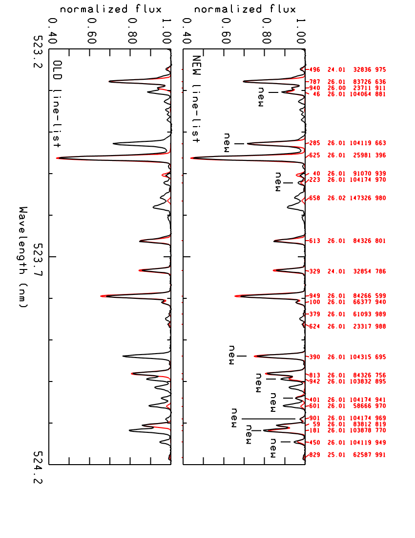
Figure 8: Comparison of the UVES spectrum of HR 6000 with a synthetic spectrum computed after this study (upper plot) and before this study (lower plot). The black line is the observed spectrum, the red line is the synthetic spectrum. Nine Fe ii lines corresponding to (³H)4d $-$ (³H)4f new identified transitions are marked in the upper plot. Their calculated $\log\,gf$’s were used for the synthetic spectrum.

Table 6: More new Fe ii identified lines

$\lambda$(obs)	$\lambda$(calc)		Lower level		Upper level		$\log\,gf$
Å	Å			cm-1		cm-1	stellar	calc.
4042.72	4042.741	K	(4P)4s4p(3P) 6P5/2	89444.458	(5D)6d 6D7/2	114173.163	$-$1.035	$-$1.243
4123.65	4123.667	K	(5D)5p 6D9/2	88723.400	(5D)6d 6P7/2	112966.820	$-$1.453	$-$1.996
4145.98	4145.922	K	(5D)5p 6D7/2	88853.533	(5D)6d 6P7/2	112966.820	$-$1.741	$-$1.847
4187.72	4187.733	K	(5D)5p 6F7/2	90300.625	(5D)6d 6D7/2	114173.163	$-$1.177	$-$1.505
$--$	4192.154	K	(5D)5p 6D5/2	89119.457	(5D)6d 6P7/2	112966.820	$-$1.882	$-$2.153
5039.704	5039.700	J	b(3F)4p 4D7/2	93129.900	(5D)6d 6P7/2	112966.820	$-$0.559	$-$5.578
5129.929	5129.915	J	(4D)4s4p 6P5/2	94685.090	(5D)6d 6D7/2	114173.163	$-$0.285	$-$4.251
5131.450	5131.445	J	b(3F)4p u4F9/2	93484.580	(5D)6d 6P7/2	112966.820	$-$1.112	$-$7.130
5134.070	5134.014	K	(3P)4p 2D5/2	94700.660	(5D)6d 6D7/2	114173.163	$-$0.225	$-$5.483

5.2 More new Fe ii identified lines

There are a few other lines not belonging to the (³H)4d-(³H)4f transitions that were identified by S. Johansson in HR 6000. They are indicated with a “J” in Table 6. The lines marked with a “K” were then obtained from predicted lines ^, thanks to the coincidence of the term of the upper predicted level with the term of a “J” line. Table 6 shows that we fixed 2 new (⁵D)6d levels. Some computed $\log\,gf$’s are much weaker than the stellar ones. Probably, some unknown transition is the main component of the observed lines so that the stellar $\log\,gf$’s are not reliable values.

6 Conclusions

Figure 8 compares synthetic spectra for HR 6000 computed before and after the study presented in this paper. The interval plotted in the figure is a significant example of the whole 5100-5400 Å region. It shows that as many as nine new Fe ii lines have been identified in 10 Å range. Nevertheless, there are still several unidentified absorptions that are probably due to Fe ii whose levels have still to be fixed. A very similar plot was obtained for 46 Aql. We can infer that a large part of the unidentified lines observed in the spectra of B-type stars are due to unknown high-excitation Fe ii transitions.

The new lines identified in this paper correspond to high excitation transitions of Fe ii with upper level just below the ionization limit. We have fixed 21 new levels of Fe ii with energies between 122910.9 cm^-1 and 123441.1 cm^-1 and we have added 1700 lines to the Fe ii linelist in the range 810 $-$15011 Å. Furthermore, Johansson (2009) identified in the spectrum of HR 6000 other Fe ii lines with lower level near the ionization limit and upper level above it, the multiplet 4s4d⁸D $-$ 4s4f⁸F at 4410 Å.

Among the new identified high-excitation Fe ii lines, several have residual flux in HR 6000 and 46 Aql as deep as 0.7 and numerous other can be observed as weak absorptions or part of blends. The two stars are iron overabundant stars, but these lines are present with lower intensity also in the UVES spectrum of HD 175640, a B-type peculiar star with an iron underabundance of $-$0.25 dex in respect to the sun (Castelli & Hubrig 2004). This fact implies that Fe ii lines from the new high excitation levels contribute to the spectrum of all Population I late B-type stars even when their abundance is less than solar. The lines are clearly observable in high resolution, high signal-to-noise spectra of slow rotating stars, while they contribute to the broad observed features in B-type stars with high rotational velocities. In general, they would appear in any object with strong Fe ii lines.

We conclude that we have clarified the nature of several unidentified lines observed in the optical spectra of B-type stars and mostly concentrated in the 5000-5400 Å region (see also Wahlgren et al.  2000), but that a large amount of work has still to be done to well reproduce stellar observations. More than 1000 energy levels of Fe ii are known, but we have seen that they are not enough. Ignorance of them and of the involved transitions is still a surviving shortcoming affecting the model atmosphere and synthetic spectra computations.

Appendix A The Balmer lines of HR 6000 observed on the UVES spectra

Figure A.1 shows the UVES spectra of HR 6000 reduced by the UVES pipeline Data Reduction Software (version 2.5; Ballester et al. 2000) that were used by Castelli & Hubrig (2007) and also in this paper. All spectra are FLUXCAL_-SCIENCE products. Those at $\lambda\lambda$ 3290-4520 Å and 4780-5650 Å are flux-calibrated spectra in 10^-16 erg s^-1 cm^-2 A^-1 corrected for terrestrial extinction. The red spectrum at 5730-7560 Å is in non-physical units ’quasi-ADU’ in that the flux calibration procedure is not implemented in the reduction software for the REDL and REDU data taken with the red mosaic CCD’s. The rather impressive distorsions of the UVES spectra make evident the difficulty in drawing a true continuum over H_γ and H_δ. Also the use of H_β produces troubles due to the position of this line at the left end of the spectrum order. Only H_α does not show manifest problems.

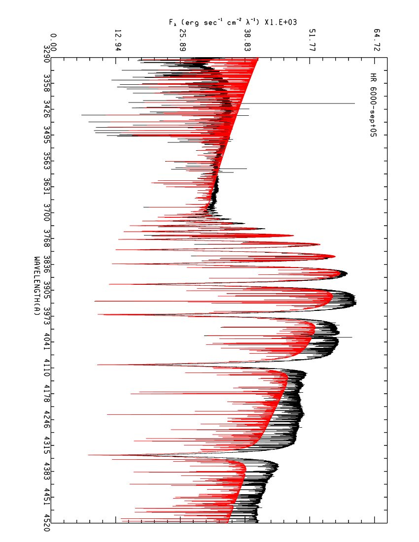
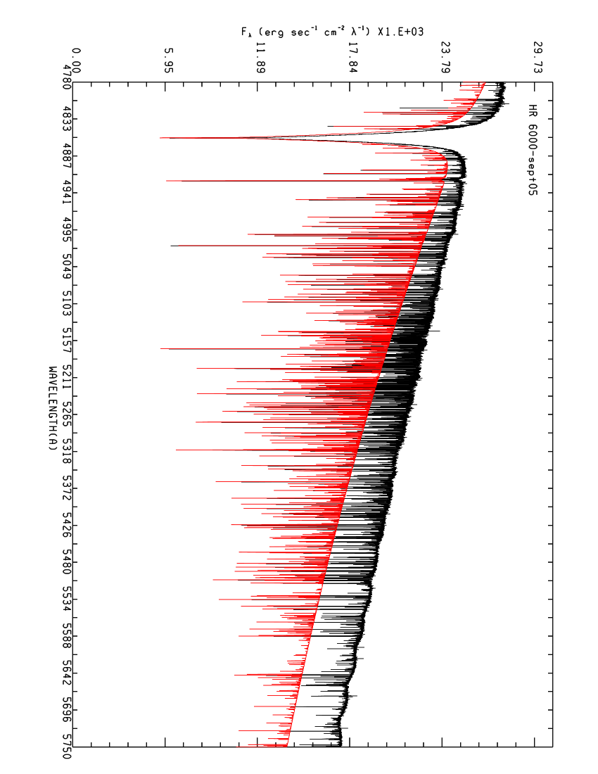
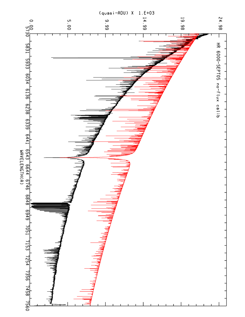
Figure 9: The observed UVES spectra of HR 6000 (black line) are plotted together the computed spectra (red line) in order to show the different slopes of the observed and computed continua. The computed fluxes are scaled by a given arbitrary quantity to be roughly overimposed on the UVES spectra. The ATLAS12 final model with parameters $T_{\rm eff}$=13450 K, $\log\,g$=4.3 was used for the computations.

Computed spectra from the final ATLAS12 model ([13450,4.3],Sect. 2.2) are also plotted in Fig. A.1 in order to show the different slopes of the observed and computed continua. The computed fluxes were scaled by a given arbitrary quantity to be roughly overimposed on the UVES spectra.

Appendix B Lines used for the abundance analysis

Table B.1 lists the lines that were examined in the spectra of HR 6000 and 46 Aql in order to derive the stellar abundances. The wording “not obs” is given for lines not present in the spectra, while the wordings “profile” and “blend” are given for lines well observed in the spectra, but which do not have measurable equivalent widths either because they are too weak to be measurable or because other components affects the line. These wording also indicate lines for which adequate equivalent widths can not be computed as in the cases of Mg ii at 4481 Å and of most O i lines which are blends of transitions belonging to the same multiplet. The abundances from the final ATLAS12 models derived from the equivalent widths or from the profiles are given in the Table, as well as upper abundance limits from lines not observed, but predicted for solar abundance by the synthetic spectrum. For Fe i and Fe ii, $\log\,gf$’s were taken from Fuhr & Wiese (2006) (FW06) when available. Otherwise Kurucz’s last detrmination was adopted (Kurucz, 2009), except for Fe ii at 5257.119 Å. In this case the previous values (Kurucz, 2007) produces synthetic profiles in better agreement with the observations.

Table 7: Analyzed lines in the stellar spectra, measured equivalent widths in mÅ, and relative abundances.He i is not included.

					HR 6000[13450,4.3,AT12]		46 Aql[12560,3.8,AT12]
Species	$\lambda$($\AA$)	$\log\,gf$	Ref.a	$\chi_{low}$	W(m$\AA$)	$log(N_{elem}/N_{\rm tot}$)	W(m$\AA$)	$log(N_{elem}/N_{\rm tot}$)
Be ii	3130.420	$-$0.170	NIST3	0.00	26.7	$-$9.78	31.0	$-$9.91
C ii	4267.001	$+$0.562	NIST3	145549.270	profile	$-$5.50	profile	$-$4.75
C ii	4267.261	$+$0.716	NIST3	145550.700	profile	$-$5.50	profile	$-$4.75
N i	8680.282	$+$0.347	NIST3	83364.620	not obs	$\leq$$-$5.80	not obs	$\leq$$-$5.50
N i	8683.403	$+$0.087	NIST3	88317.830	not obs	$\leq$$-$5.80	not obs	$\leq$$-$5.50
O i	3947.295	$-$2.095	NIST3	73768.200	profile	$-$3.71	profile	$-$3.71
O i	3947.481	$-$2.244	NIST3	73768.200	profile	$-$3.71	profile	$-$3.71
O i	3947.586	$-$2.467	NIST3	73768.200	profile	$-$3.71	profile	$-$3.71
O i	4368.193	$-$2.665	NIST3	76794.978	profile	$-$3.71	profile	$-$3.51
O i	4368.242	$-$1.964	NIST3	76794.978	profile	$-$3.71	profile	$-$3.51
O i	4368.258	$-$2.186	NIST3	76794.978	profile	$-$3.71	profile	$-$3.51
O i	5329.096	$-$1.938	NIST3	86625.757	profile	$-$3.71	profile	$-$3.46
O i	5329.099	$-$1.586	NIST3	86625.757	profile	$-$3.71	profile	$-$3.46
O i	5329.107	$-$1.695	NIST3	86625.757	profile	$-$3.71	profile	$-$3.46
O i	6155.961	$-$1.363	NIST3	86625.757	profile	$-$3.64	profile	$-$3.46
O i	6155.971	$-$1.011	NIST3	86625.757	profile	$-$3.64	profile	$-$3.46
O i	6155.989	$-$1.120	NIST3	86625.757	profile	$-$3.64	profile	$-$3.46
O i	6156.737	$-$1.487	NIST3	86627.778	profile	$-$3.64	profile	$-$3.43
O i	6156.755	$-$0.898	NIST3	86627.778	profile	$-$3.64	profile	$-$3.43
O i	6156.778	$-$0.694	NIST3	86627.778	profile	$-$3.64	profile	$-$3.43
O i	6455.977	$-$0.920	NIST3	86631.454	profile	$-$3.59	profile	$-$3.43
O i	7002.196	$-$1.489	NIST3	88631.146	profile	$-$3.71	H2O	$--$
O i	7002.230	$-$0.741	NIST3	88631.146	profile	$-$3.71	H2O	$--$
O i	7002.250	$-$1.364	NIST3	88631.303	profile	$-$3.71	H2O	$--$
Ne i	7032.413	$-$0.249	NIST3	134041.840	noise?	$-$4.86	noise ?	$-$4.51
Na i	5688.205	$-$0.452	NIST3	16973.368	not obs	$\leq$$-$5.71	profile	$-$5.65
Na i	5889.950	$+$0.108	NIST3	0.00	inters.	$--$	profile	$-$5.67
Na i	5895.924	$-$0.194	NIST3	0.00	inters.	$--$	profile	$-$5.72
Mg ii	4481.126	$+$0.749	NIST3	71490.190	profile	$-$5.66	profile	$-$5.45
Mg ii	4481.150	$-$0.553	NIST3	71490.190	profile	$-$5.66	profile	$-$5.45
Mg ii	4481.325	$+$0.594	NIST3	71491.063	profile	$-$5.66	profile	$-$5.45
Al i	3944.006	$-$0.638	NIST3	0.000	not obs	$\leq$$-$7.30	not obs	$\leq$$-$6.65
Al i	3961.520	$-$0.336	NIST3	112.061	not obs	$\leq$$-$7.30	profile	$-$6.65
Al ii	7042.083	$+$0.340	NIST3	91274.500	noise ?	$\leq$$-$7.30	noise ?	$\leq$$-$7.40
Al ii	7056.712	$+$0.110	NIST3	91274.500	noise ?	$\leq$$-$7.30	noise ?	$\leq$$-$7.00
Si ii	3853.665	$-$1.341	NIST3	55309.350	not obs	$--$	31.8	$-$5.62
Si ii	3862.595	$-$0.406	NIST3	55325.180	not obs	$--$	71.8	$-$5.68
Si ii	3862.595	$-$0.757	NIST3	55309.350	profile	$-$7.35	62.6	$-$5.53
P ii	4044.576	$+$0.481	K,MRB	107360.250	45.3	$-$4.42	19.9	$-$5.16
P ii	4062.149	$-$0.585	K,MRB	103339.140	8.6	$-$4.79	2.4	$-$5.45
P ii	4127.559	$-$0.110	K,KP	103667.860	25.2	$-$4.54	9.3	$-$5.21
P ii	4160.623	$-$0.410	K,KP	103339.140	9.4	$-$4.90	7.6	$-$5.03
P ii	4244.622	$-$0.308	K,MRB	107360.250	9.6	$-$4.78	2.6	$-$5.46
P ii	4288.606	$-$0.630	K,MRB	101635.690	7.0	$-$4.88	blend	$--$
P ii	4420.712	$-$0.329	NIST3	88893.220	40.1	$-$4.51	19.4	$-$5.18
P ii	4452.472	$-$0.194	K,MRB	105302.170	19.9	$-$4.48	6.9	$-$5.13
P ii	4463.027	$+$0.026	K,MRB	105549.670	25.6	$-$4.52	9.1	$-$5.19
P ii	4466.140	$-$0.560	NIST3	105549.670	9.8	$-$4.57	2.2	$-$5.32
P ii	4468.000	$-$0.208	K,MRB	105244.060	24.0	$-$4.35	blend	$--$
P ii	4475.270	$+$0.440	NIST3	105549.670	36.8	$-$4.63	16.2	$-$5.25
P ii	4483.693	$-$0.431	NIST3	105302.370	10.0	$-$4.69	2.3	$-$5.43
P ii	4499.230	$+$0.470	NIST3	107922.930	38.0	$-$4.44	blend	$--$
P ii	5296.077	$-$0.160	NIST3	87124.600	56.3	$-$4.15	33.9	$-$4.74
P ii	5316.055	$-$0.294	NIST3	86743.960	47.9	$-$4.31	28.3	$-$4.82
P ii	5344.729	$-$0.390	NIST3	86597.550	45.6	$-$4.28	25.7	$-$4.81
P ii	5386.895	$-$0.520	NIST3	86743.960	51.8	$-$3.98	25.6	$-$4.67
P ii	5425.880	$+$0.180	NIST3	87124.600	71.8	$-$4.22	47.4	$-$4.71

Table 1: cont.

					HR 6000[13450,4.3,AT12]		46 Aql[12560,3.8,AT12]
Species	$\lambda$($\AA$)	$\log\,gf$	Ref.a	$\chi_{low}$	W(m$\AA$)	$log(N_{elem}/N_{\rm tot}$)	W(mÅ)	$log(N_{elem}/N_{\rm tot}$)
P ii	6024.178	$+$0.137	NIST3	86743.960	69.8	$-$4.04	45.7	$-$4.57
P ii	6034.039	$-$0.220	NIST3	86597.550	52.6	$-$4.10	29.4	$-$4.70
P ii	6043.084	$+$0.416	NIST3	87124.600	81.1	$-$4.05	55.5	$-$4.57
P iii	4059.312	$-$0.051	NIST3	116885.870	11.1	$-$4.97	2.5	$-$5.87
P iii	4080.089	$-$0.306	NIST3	116874.560	5.5	$-$5.21	not ob	$--$
P iii	4222.198	$+$0.210	NIST3	117835.950	19.5	$-$5.45	not obs	$--$
P iii	4246.720	$-$0.120	NIST3	117835.950	10.6	$-$4.78	not obs	$--$
S ii	4162.665	$+$0.777	NIST3	128599.160	2.0	$-$6.26	5.3	$-$5.74
Cl i	4794.556	$+$0.400	NIST3	107879.660	not obs	$\leq$$-$7.24	not obs	$\leq$$-$7.04
Ca i	4226.728	$+$0.244	NIST3	0.000	profile	$>$$-$5.68	profile	$>$$-$5.98
Ca ii	3933.663	$+$0.135	NIST3	0.000	profile	$-$5.68	profile	$-$5.98
Ca ii	3968.469	$-$0.180	NIST3	0.000	profile	$-$5.68	profile	$-$5.98
Sc ii	4246.822	$+$0.242	NIST3	2540.950	blend	$--$	blend	$--$
Sc ii	4314.083	$-$0.100	NIST3	4987.790	not obs	$\leq$ $-$9.50	not obs	$\leq$$-$9.50
Ti ii	4053.821	$-$1.130	PTP	15265.620	6.4	$-$6.40	11.1	$-$6.46
Ti ii	4163.644	$-$0.130	PTP	20891.660	19.3	$-$6.51	30.4	$-$6.50
Ti ii	4287.873	$-$1.790	PTP	8710.440	3.5	$-$6.38	6.1	$-$6.49
Ti ii	4290.215	$-$0.850	PTP	9395.710	15.6	$-$6.55	28.3	$-$6.52
Ti ii	4294.094	$-$0.930	PTP	9744.250	16.5	$-$6.47	28.3	$-$6.48
Ti ii	4300.042	$-$0.440	PTP	9518.060	30.2	$-$6.52	45.2	$-$6.49
Ti ii	4301.922	$-$1.150	PTP	9363.620	8.6	$-$6.56	17.1	$-$6.55
Ti ii	4367.652	$-$0.860	PTP	20891.660	5.7	$-$6.42	9.9	$-$6.46
Ti ii	4395.031	$-$0.540	PTP	8744.250	29.2	$-$6.49	45.2	$-$6.43
Ti ii	4399.765	$-$1.190	PTP	9975.920	3.3	$-$6.94	17.2	$-$6.48
Ti ii	4411.072	$-$0.670	PTP	24961.030	5.0	$-$6.45	10.1	$-$6.40
Ti ii	4417.714	$-$1.190	PTP	9395.710	8.8	$-$6.51	16.4	$-$6.54
Ti ii	4418.331	$-$1.970	PTP	9975.920	2.4	$-$6.31	3.5	$-$6.50
Ti ii	4443.810	$-$0.720	PTP	8710.440	22.3	$-$6.50	37.1	$-$6.47
Ti ii	4450.482	$-$1.520	PTP	8744.250	5.5	$-$6.45	11.5	$-$6.44
Ti ii	4464.448	$-$1.810	PTP	9363.620	3.1	$-$6.40	6.8	$-$6.38
Ti ii	4468.492	$-$0.620	NIST3	9118.260	25.6	$-$6.50	39.6	$-$6.50
Ti ii	4488.325	$-$0.510	PTP	25192.710	7.0	$-$6.44	12.4	$-$6.44
Ti ii	4501.270	$-$0.770	PTP	8997.710	23.0	$-$6.41	37.6	$-$6.39
Ti ii	4805.085	$-$1.120	NIST3	16625.110	7.2	$-$6.28	14.5	$-$6.27
Ti ii	4911.195	$-$0.610	PTP	25192.790	5.4	$-$6.45	10.7	$-$6.42
V ii	3093.105	$+$0.530	K,NBS	3162.800	blend	$\leq$$-$9.14	noise ?	$\leq$$-$8.94
V ii	3102.289	$+$0.410	K,NBS	2968.220	not obs	$\leq$$-$9.14	noise	$\leq$$-$8.94
V ii	3110.695	$+$0.300	K,NBS	2808.720	blend	$\leq$$-$9.14	blend	$\leq$$-$8.94
V ii	3113.376	$+$0.180	K,NBS	2687.010	not obs	$\leq$$-$9.14	not obs	$\leq$$-$8.94
V ii	3125.276	$+$0.070	K,NBS	2604.820	blend	$\leq$$-$9.14	blend	$-$8.94
Cr ii	4812.337	$-$1.800	NIST3	31168.580	3.7	$-$6.21	not obs	$--$
Cr ii	4824.127	$-$0.970	SL	31219.350	26.4	$-$5.98	blend	$--$
Cr ii	4836.229	$-$2.000	SL	31117.390	3.9	$-$5.99	not obs	$--$
Cr ii	5237.329	$-$1.160	NIST3	32854.310	12.5	$-$6.16	1.5	$-$7.48
Cr ii	5246.768	$-$2.460	NIST3	29951.880	1.2	$-$6.14	not obs	$--$
Mn ii	3441.988	$-$0.270	NIST3	14325.860	85.3	$-$4.92 ($-$5.00)b	74.5	$-$5.48 ($-$5.35)b
Mn ii	3460.316	$-$0.540	NIST3	14593.820	74.5	$-$4.91 ($-$5.00)	60.2	$-$5.65 ($-$5.65)
Mn ii	3482.905	$-$0.740	NIST3	14781.190	65.3	$-$4.98 ($-$5.00)	53.0	$-$5.70 ($-$5.65)
Mn ii	3488.677	$-$0.860	NIST3	14901.180	65.7	$-$4.85 ($-$4.85)	52.5	$-$5.60 ($-$5.60)
Mn ii	3495.833	$-$1.220	NIST3	14959.840	55.3	$-$4.85 ($-$4.85)	42.2	$-$5.65 ($-$5.65)
Mn ii	3496.809	$-$1.690	NIST3	14781.190	38.1	$-$5.09 ($-$5.00)	27.0	$-$5.87 ($-$5.90)
Mn ii	3497.526	$-$1.330	NIST3	14901.180	47.7	$-$5.05 ($-$4.90)	35.5	$-$5.84 ($-$5.85)
Mn ii	3917.318	$-$1.169	K03Mn	55759.270	4.9	$-$5.61 ($-$5.65)	2.8	$-$6.09 ($-$6.17)
Mn ii	4363.258	$-$1.929	K03Mn	44899.820	4.2	$-$5.49 ($-$5.58)	2.3	$-$6.03 ($-$6.15)
Mn ii	4365.219	$-$1.339	K03Mn	44899.820	4.7	$-$5.59 ($-$5.63)	3.1	$-$6.02 ($-$6.07)
Mn ii	4478.635	$-$0.942	K03Mn	53597.130	8.2	$-$5.68 ($-$5.63)	5.0	$-$6.16 ($-$6.15)
Fe i	3581.193	$+$0.406	FW06	6928.27	17.3	$-$3.67	19.2	$-$3.86
Fe i	3618.768	$-$0.003	FW06	7985.78	8.0	$-$3.73	10.3	$-$3.88
Fe i	4005.242	$-$0.610	FW06	12560.93	6.6	$-$3.59	6.4	$-$3.94

Table 1: cont.

					HR 6000[13450,4.3,AT12]		46 Aql[12560,3.8,AT12]
Species	$\lambda$($\AA$)	$\log\,gf$	Ref.a	$\chi_{low}$	W(m$\AA$)	$log(N_{elem}/N_{\rm tot}$)	W(m$\AA$)	$log(N_{elem}/N_{\rm tot}$)
Fe i	4071.738	$-$0.022	FW06	12698.55	15.4	$-$3.71	17.0	$-$3.99
Fe i	4202.029	$-$0.708	FW06	11976.24	4.5	$-$3.71	5.7	$-$3.93
Fe i	4219.360	$+$0.000	FW06	28819.95	4.0	$-$3.55	4.4	$-$3.78
Fe i	4235.936	$-$0.341	FW06	19562.44	4.9	$-$3.62	5.9	$-$3.84
Fe i	4271.760	$-$0.164	FW06	11976.24	14.7	$-$3.66	16.4	$-$3.93
Fe i	4383.545	$+$0.200	FW06	11976.24	25.2	$-$3.67	27.6	$-$3.95
Fe i	4404.750	$-$0.142	FW06	12560.93	18.6	$-$3.51	18.0	$-$3.87
Fe i	4415.122	$-$0.615	FW06	12968.55	6.2	$-$3.61	8.0	$-$3.81
Fe i	5324.179	$-$0.103	FW06	25899.99	blend	$--$	3.3	$-$3.98
Fe i	5364.871	$+$0.228	FW06	35856.40	2.4	$-$3.61	2.2	$-$3.92
Fe i	5369.962	$+$0.536	FW06	35257.32	5.0	$-$3.62	4.3	$-$3.95
Fe i	5410.910	$+$0.398	FW06	36079.37	2.6	$-$3.74	2.9	$-$3.94
Fe i	5424.068	$+$0.580	FW06	34843.95	blend	$--$	5.0	$-$3.94
Fe i	5615.644	$+$0.050	FW06	26874.55	blend	$--$	3.9	$-$3.99
Fe ii	3906.035	$-$1.700	FW06	44929.55	42.8	$-$3.82	43.7	$-$4.02
Fe ii	3914.503	$-$4.370	FW06	13473.41	18.1	$-$3.60	22.4	$-$3.80
Fe ii	3935.962	$-$1.720	FW06	44915.05	43.3	$-$3.79	44.1	$-$3.99
Fe ii	3938.290	$-$4.070	FW06	13471.41	37.1	$-$3.35	31.7	$-$3.83
Fe ii	3945.210	$-$4.440	FW06	13673.18	14.7	$-$3.65	18.1	$-$3.85
Fe ii	4122.668	$-$3.300	FW06	20830.58	33.4	$-$3.82	36.8	$-$4.03
Fe ii	4128.748	$-$3.580	FW06	20830.58	23.6	$-$3.82	27.9	$-$4.00
Fe ii	4178.862	$-$2.440	FW06	20830.58	58.3	$-$3.93	61.7	$-$4.11
Fe ii	4258.154	$-$3.480	FW06	21812.05	26.6	$-$3.78	29.7	$-$3.99
Fe ii	4273.326	$-$3.300	FW06	21812.05	32.6	$-$3.79	39.6	$-$3.90
Fe ii	4296.572	$-$2.930	FW06	21812.05	44.5	$-$3.82	50.1	$-$3.95
Fe ii	4303.176	$-$2.610	FW06	21812.05	57.6	$-$3.74	63.1	$-$3.86
Fe ii	4369.411	$-$3.580	FW06	22409.85	21.5	$-$3.80	25.5	$-$3.98
Fe ii	4413.601	$-$4.190	FW06	21581.64	10.4	$-$3.66	13.7	$-$3.81
Fe ii	4416.830	$-$2.600	FW06	22409.85	56.7	$-$3.75	59.3	$-$3.96
Fe ii	4491.405	$-$2.640	FW06	23031.30	49.8	$-$3.88	53.5	$-$4.06
Fe ii	4508.288	$-$2.350	FW06	23031.30	66.2	$-$3.68	70.1	$-$3.84
Fe ii	4515.339	$-$2.360	FW06	23939.36	57.8	$-$3.86	61.3	$-$4.04
Fe ii	4520.224	$-$2.620	FW06	22637.21	54.4	$-$3.78	no spectra	$--$
Fe ii	4522.634	$-$1.990	FW06	22939.36	68.7	$-$3.97	no spectra	$--$
Fe ii	4923.927	$-$1.210	FW06	23317.63	100.8	$-$3.91	blend	$--$
Fe ii	4993.358	$-$3.680	FW06	22637.20	19.6	$-$3.74	23.2	$-$3.93
Fe ii	5004.188	$+$0.482	K09	82853.66			47.6	$-$3.88
Fe ii	5006.840	$-$0.281	K09	83713.53			20.4	$-$3.90
Fe ii	5007.450	$-$0.382	K09	83726.37			16.4	$-$3.94
Fe ii	5010.060	$-$0.808	K09	83726.37			10.1	$-$3.80
Fe ii	5011.026	$-$1.177	K09	83726.37			3.6	$-$3.95
Fe ii	5018.440	$-$1.350	FW06	23317.63	111.7	$-$3.57	116.7	$-$3.77
Fe ii	5022.419	$-$0.052	K09	83459.67			23.6	$-$4.03
Fe ii	5026.798	$-$0.235	K09	83136.46			22.0	$-$3.92
Fe ii	5030.631	$+$0.431	FW06	82978.68	50.7	$-$3.69	43.2	$-$3.95
Fe ii	5032.704	$+$0.143	K09	83812.30			30.9	$-$3.97
Fe ii	5035.700	$+$0.630	FW06	82978.68	59.7	$-$3.64	51.6	$-$3.90
Fe ii	5036.713	$-$0.527	K09	83812.30			13.0	$-$3.94
Fe ii	5045.108	$-$0.116	K09	83136.46			26.8	$-$3.88
Fe ii	5060.249	$-$0.479	K09	84266.54			12.7	$-$3.97
Fe ii	5062.927	$-$1.166	K09	83136.46			7.0	$-$3.68
Fe ii	5067.890	$-$0.173	K09	83308.19			22.4	$-$3.95
Fe ii	5070.583	$-$0.865	K09	83308.19			6.6	$-$3.99
Fe ii	5070.895	$+$0.262	K09	83136.46			37.9	$-$3.92
Fe ii	5075.760	$+$0.233	K09	84326.92			33.3	$-$3.95
Fe ii	5076.597	$-$0.749	K09	83713.53			8.8	$-$3.95
Fe ii	5081.898	$-$0.689	K09	83713.53			8.3	$-$4.02

Table 1: cont.

					HR 6000[13450,4.3,AT12]		46 Aql[12560,3.8,AT12]
Species	$\lambda$($\AA$)	$\log\,gf$	Ref.a	$\chi_{low}$	W(m$\AA$)	$log(N_{elem}/N_{\rm tot}$)	W(m$\AA$)	$log(N_{elem}/N_{\rm tot}$)
Fe ii	5086.306	$-$0.472	K09	83990.06			14.7	$-$3.90
Fe ii	5089.214	$-$0.014	K09	83308.19			27.0	$-$3.96
Fe ii	5093.783	$-$0.703	K09	83726.37			12.7	$-$3.77
Fe ii	5117.032	$-$0.129	K09	84131.58			22.0	$-$3.96
Fe ii	5132.669	$-$4.090	FW06	22637.20	17.5	$-$3.40	14.0	$-$3.83
Fe ii	5140.692	$-$0.822	K09	83990.06			9.9	$-$3.78
Fe ii	5143.875	$+$0.054	K09	84266.54			21.6	$-$4.14
Fe ii	5144.352	$+$0.307	FW06	84424.37	40.1	$-$3.73	32.8	$-$4.03
Fe ii	5169.033	$-$0.870	FW06	23317.63	115.1	$-$4.01	121.0	$-$4.19
Fe ii	5180.312	$+$0.002	K09	83812.30			26.9	$-$3.94
Fe ii	5199.118	$+$0.054	K09	83713.53			30.3	$-$3.87
Fe ii	5200.798	$-$0.390	K09	83812.30			17.4	$-$3.87
Fe ii	5203.634	$-$0.088	K09	83812.30			25.9	$-$3.88
Fe ii	5218.841	$-$0.250	K09	83726.37			23.6	$-$3.85
Fe ii	5219.920	$-$0.628	K09	84870.86			10.3	$-$3.89
Fe ii	5222.350	$-$0.332	K09	84844.82			15.0	$-$3.96
Fe ii	5223.802	$-$0.546	K09	83713.53			14.6	$-$3.83
Fe ii	5224.404	$-$0.581	K09	83990.06			12.5	$-$3.87
Fe ii	5234.625	$-$2.210	FW06	25981.63	69.6	$-$3.54	71.0	$-$3.76
Fe ii	5237.949	$+$0.103	K09	84266.54			29.8	$-$3.90
Fe ii	5245.455	$-$0.502	K09	84326.92			13.6	$-$3.88
Fe ii	5247.956	$+$0.550	FW06	84938.18	46.2	$-$3.74	39.7	$-$4.01
Fe ii	5257.119	$+$0.115	K07	84685.20			26.7	$-$4.00
Fe ii	5265.985	$-$0.936	K09	84035.12			9.3	$-$3.68
Fe ii	5270.029	$-$0.097	K09	84710.70			18.0	$-$4.08
Fe ii	5272.397	$-$2.010	FW06	48039.09	35.0	$-$3.51	35.4	$-$3.71
Fe ii	5276.002	$-$1.900	FW06	25805.33	67.0	$-$3.93	71.7	$-$4.07
Fe ii	5284.109	$-$3.200	FW06	23317.63	38.2	$-$3.63	40.6	$-$3.86
Fe ii	5291.661	$+$0.561	K09	84527.76			42.8	$-$3.95
Fe ii	5306.182	$+$0.044	FW06	84870.87	30.4	$-$3.70	26.7	$-$3.91
Fe ii	5315.083	$-$0.422	K09	85048.61			13.2	$-$3.93
Fe ii	5316.615	$-$1.780	FW06	25428.78	79.9	$-$3.71	81.9	$-$3.93
Fe ii	5318.055	$-$0.177	K09	84527.76			22.3	$-$3.85
Fe ii	5355.421	$-$0.203	K09	84685.20			13.2	$-$4.17
Fe ii	5358.872	$-$0.130	K09	84685.20			14.8	$-$4.17
Fe ii	5359.237	$-$1.112	K09	84710.70			7.2	$-$3.59
Fe ii	5366.210	$-$0.549	K09	84710.70			16.4	$-$3.68
Fe ii	5425.257	$-$3.390	FW06	25805.33	27.8	$-$3.59	30.2	$-$3.81
Fe ii	5430.003	$+$0.427	FW06	85462.86			36.7	$-$3.92
Fe ii	5444.386	$-$0.153	K09	85495.32			19.5	$-$3.90
Fe ii	5451.316	$-$0.756	K09	84685.20			7.1	$-$3.95
Fe ii	5465.932	$+$0.348	FW06	85679.70	42.3	$-$3.58	35.6	$-$3.86
Fe ii	5472.855	$-$0.723	K09	84685.20			10.5	$-$3.77
Fe ii	5475.826	$-$0.129	K09	84685.20			19.7	$-$3.96
Fe ii	5488.776	$-$0.468	K09	85462.86			13.3	$-$3.84
Fe ii	5492.398	$-$0.127	K09	84685.20			25.1	$-$3.78
Fe ii	5493.830	$+$0.259	FW06	84685.20	37.7	$-$3.68	32.5	$-$3.93
Fe ii	5502.670	$-$0.179	K09	85184.73			21.2	$-$3.83
Fe ii	5534.847	$-$2.860	FW06	26170.18	50.5	$-$3.44	51.1	$-$3.70
Co ii	3501.708	$-$1.111	K06	17771.506	not obs	$--$	not obs	$\leq$ $-$8.02
Co ii	4160.657	$-$1.751	K06	27484.371	blend	$--$	blend	$--$
Ni ii	4067.031	$-$1.834	K03Ni	32499.530	9.9	$-$6.24	9.8	$-$6.47
Cu ii	4909.734	$+$0.790	K03Cu	115568.985	not obs	$--$	3.1	$-$6.26
Cu ii	4931.698	$+$0.704	K03Cu	115662.550	not obs	$--$	2.7	$-$6.22
Zn i	4810.528	$-$0.137	K,WAR	32890.352	not obs	$--$	5.1	$-$5.85
Zn ii	4911.625	$+$0.540	NIST3	96909.740	not obs	$--$	23.0	$-$5.76

Table 1: cont.

					HR 6000[13450,4.3,AT12]		46 Aql[12560,3.8,AT12]
Species	$\lambda$($\AA$)	$\log\,gf$	Ref.a	$\chi_{low}$	W(m$\AA$)	$log(N_{elem}/N_{\rm tot}$)	W(m$\AA$)	$log(N_{elem}/N_{\rm tot}$)
Ga ii	4255.722	$+$0.634	RS94	113842.190	not obs	$--$	not obs	$--$
Ga ii	6334.069	$+$1.000	RS94	102944.550	not obs	$--$	not obs	$--$
As ii	5105.58	$--$	$--$	81508.925	not obs	$--$	4.0	$--$
As ii	5107.55	$--$	$--$	82819.214	not obs	$--$	blend	$--$
As ii	5231.38	$--$	$--$	79128.330	not obs	$--$	3.2	$--$
As ii	5331.23	$--$	$--$	81508.925	not obs	$--$	9.4	$--$
As ii	5497.73	$--$	$--$	78730.893	not obs	$--$	blend	$--$
As ii	5558.09	$--$	$--$	79128.330	not obs	$--$	9.4	$--$
As ii	5651.32	$--$	$--$	81508.925	not obs	$--$	11.0	$--$
As ii	6110.07	$--$	$--$	83819.214	not obs	$--$	3.3	$--$
As ii	6170.27	$--$	$--$	79128.330	not obs	$--$	blend	$--$
Sr ii	4077.709	$+$0.151	NIST3	0.000	not obs	$--$	not obs	$--$
Y ii	3950.349	$-$0.490	K,HL	840.213	profile	$-$8.60	4.2	$-$8.20
Y ii	4883.682	$+$0.070	K,HL	8743.316	profile	$-$8.60	7.3	$-$8.03
Y ii	4900.120	$-$0.090	K,HL	8328.041	profile	$-$8.60	5.5	$-$8.04
Xe ii	4844.330	$+$0.491	NIST3	93068.440	28.8	$-$5.23	17.5	$-$5.81
Hg ii	3983.890	$-$1.510	NIST3	35514.000	profile	$-$8.20	profile	$-$7.10

^a (NIST3) NIST Atomic Spectra Database, version 3 at http://physics.nist.gov;
(FW06) Fuhr & Wiese (2006);
(PTP) Pickering et al. (2002);
(RS94) Ryabchikova & Smirnov (1994);
(SL) Sigut & Landstreet (1990);
K03Mn: http://kurucz.harvard.edu/atoms/2501/gf2501.pos;
K03Ni: http://kurucz.harvard.edu/atoms/2801/gf2801.pos;
K03Cu: http://kurucz.harvard.edu/atoms/2901/gf2901.pos;
K06: http://kurucz.harvard.edu/atoms/2701/gf2701.pos;
K07: http://kurucz.harvard.edu/atoms/2601/gf2601.pos, 2007 version, no longer available. The $\log\,gf$ gives better agreement with the observations than the K09 new determination;
K09: http://kurucz.harvard.edu/atoms/2601/gf2601.pos,January 2009 version;
“K” before another $\log\,gf$ source means that the $\log\,gf$ is from Kurucz files available at http://kurucz.harvard.edu/linelists/gf100/; (HL) Hannaford et al. (1982);(KP) Kurucz & Peytremann (1975); (MRB) Miller et al. (1971); (NBS) Younger et al. (1979); (WAR) Warner (1968).
^b The abundances given in parenthesis were derived from line profiles. All computed line profiles include hyperfine components, except for that at 3917.318 $\AA$.

References

- Ballester et al. (2000) Ballester, P., Grosbol, P., Banse, K., Disaro, A., Dorigo, D., Modigliani, A., Pizarro de la Iglesia, J. A., & Boitquin, O. 2000, Proc. SPIE, 4010, 246
- (2) Castelli, F. 2005, MSAIS, 8, 44
- Castelli & Hubrig (2004) Castelli, F., & Hubrig, S. 2004, A&A, 425, 263
- Castelli & Hubrig (2007) Castelli, F., & Hubrig, S. 2007, A&A, 475, 1041
- Castelli et al. (2008) Castelli, F., Johansson, S., & Hubrig, S. 2008, Journal of Physics Conference Series, 130, 012003
- (6) Cowan, R. D. 1981, The Theory of Atomic Structure and Spectra (Berkeley: Univ. California Press)
- Fuhr & Wiese (2006) Fuhr, J. R., & Wiese, W. L. 2006, Journal of Physical and Chemical Reference Data, 35, 1669
- Grevesse & Sauval (1998) Grevesse, N., & Sauval, A. J. 1998, Space Science Reviews, 85, 161
- Hannaford et al. (1982) Hannaford, P., Lowe, R. M., Grevesse, N., Biemont, E., & Whaling, W. 1982, ApJ, 261, 736
- Hauck & Mermilliod (1998) Hauck, B., & Mermilliod, M. 1998, A&AS, 129, 431
- Johansson (2002) Johansson, S. 2002, Highlights of Astronomy, 12, 84
- Johansson (2009) Johansson, S. 2009, Physica Scripta, T134, 014013
- Johansson & Cowley (1984) Johansson, S., & Cowley, C. R. 1984, A&A, 139, 243
- (14) Kurucz, R. L. 1993, SYNTHE Spectrum Synthesis Programs and Line Data, CD-ROM, No. 18
- Kurucz (2005) Kurucz, R. L. 2005, Memorie della Societa’ Astronomica Italiana Supplement, 8, 14
- Kurucz & Peytremann (1975) Kurucz, R. L., & Peytremann, E. 1975, SAO Special Report, 362,
- Michaud (1970) Michaud, G. 1970, ApJ, 160, 641
- Miller et al. (1971) Miller, M. H., Roig, R. A., & Bengtson, R. D. 1971, Phys. Rev. A, 4, 1709
- Pickering et al. (2002) Pickering, J. C., Thorne, A. P., & Perez, R. 2002, ApJS, 138, 247
- Raassen & Uylings (1998) Raassen, A. J. J., & Uylings, P. H. M. 1998, A&A, 340, 300
- Ryabchikova & Smirnov (1994) Ryabchikova, T. A., & Smirnov, Y. M. 1994, Astronomy Reports, 38, 70
- Ryabchikova et al. (2003) Ryabchikova, T., Wade, G. A., & LeBlanc, F. 2003, Modelling of Stellar Atmospheres, 210, 301
- Sadakane et al. (2001) Sadakane, K., et al. 2001, PASJ, 53, 1223
- Sbordone et al. (2004) Sbordone, L., Bonifacio, P., Castelli, F., & Kurucz, R. L. 2004, Memorie della Societa Astronomica Italiana Supplement, 5, 93
- Sigut & Landstreet (1990) Sigut, T. A. A., & Landstreet, J. D. 1990, MNRAS, 247, 611
- (26) Younger, S. M., Fuhr, Y. R., Martin, G. A., & Wiese, W. L. 1978, Journal of Physical and Chemical Reference Data, 7, 495
- Wahlgren et al. (2000) Wahlgren, G. M., Dolk, L., Kalus, G., Johansson, S., Litzén, U., & Leckrone, D. S. 2000, ApJ, 539, 908
- (28) Warner, B., 1968, MNRAS, 140, 53