Thermal expansion in single-walled carbon nanotubes and graphene: nonequilibrium Green’s function approach

Abstract

The nonequilibrium Green’s function method is applied to investigate the coefficient of thermal expansion (CTE) in single-walled carbon nanotubes (SWCNT) and graphene. It is found that atoms expand about 1$\%$ from equilibrium positions even at $T=0$ K, resulting from the interplay between quantum zero-point motion and nonlinear interaction. The CTE in SWCNT of different sizes is studied and analyzed in terms of the competition between various vibration modes. As a result of this competition, the axial CTE is positive in the whole temperature range, while the radial CTE is negative at low temperatures. In graphene, the CTE is very sensitive to the substrate. Without substrate, CTE has large negative region at low temperatures and very small value at high temperature limit, and the value of CTE at 300 K is $-6\times 10^{-6}$ K^-1 which is very close to a recent experimental result, $-7\times 10^{-6}$ K^-1 [Nat. Nanotechnol. 10, 1038 (2009)]. A very weak substrate interaction (about 0.06$\%$ of the in-plane interaction) can largely reduce the negative CTE region and greatly enhance the value of CTE. If the substrate interaction is strong enough, the CTE will be positive in whole temperature range and the saturate value at high temperatures reaches $2.0\times 10^{-5}$ K^-1.

I introduction

Single-walled carbon nanotubes (SWCNT) and graphene are two kinds of novel carbon based materials with lots of intriguing electronic and mechanical properties.DaiHJ ; Dresselhaus ; Novoselov ; Avouris ; Neto ; Geim They have many potential applications in nano-devices, where the thermal property plays a big role. The coefficient of thermal expansion (CTE) is one of the most important nonlinear thermal properties. Very recently, the CTE of graphene is measured to be $-7\times 10^{-6}$ K^-1 at $T=300$ K.BaoW Also the CTE of multi-walled carbon nanotubesRuoff ; Bandow ; Maniwa1 and nanotube bundlesYosida ; Maniwa2 ; Dolbin ; Dolbin2009 are measured in experiments. Theoretically, there are several approaches to calculate CTE such as molecular dynamics,Raravikar ; Schelling ; Cao ; KwonYK lattice dynamics calculations,Schelling ; Barron ; Fabian ; Broido ; Ward the molecular structural mechanics methodLiC , analytical methodJiang , and ab initio density-functional theory and density-functional pertubation theory calculations.Mounet ; Bonini However, discrepancies exist in different approaches. In Ref. Jiang, ; Schelling, ; KwonYK, , the CTE is predicted to be negative in low temperature region while positive at high temperatures. On the contrary, Li and Chou obtain positive value for CTE in whole temperature range.LiC In Ref. Mounet, , CTE for graphite is negative at low temperatures and positive at high temperatures, and CTE for graphene is negative in whole temperature range. In Refs. Jiang, ; KwonYK, , the axial CTE increases from negative to positive with increasing temperature; while the minimum value of axial CTE is quite different: $-1\times 10^{-6}$ K^-1 or $-5\times 10^{-5}$ K^-1 and this value is achieved at different temperatures: 300 K or 500 K in Ref. Jiang, and Ref. KwonYK, respectively. In the high temperature region, the value for CTE is also quite different from one to another, typically about $2.0\times 10^{-6}$ K^-1 in Refs. LiC, ; Schelling, , $4.0\times 10^{-6}$ K^-1 in Ref. Jiang, or more than $5\times 10^{-6}$ K^-1 in Ref. KwonYK, . In Ref. LiC, the CTE shows only a slight dependence on the length or diameter of the SWCNT. While Ref. Jiang, predicts the obvious decrease of CTE with increasing diameter. To the best of our knowledge, the limited existing theoretical works are diverse.

In this paper, we investigate the CTE in SWCNT and graphene sheets by the nonequilibrium Green’s function (GF) approach, which includes contributions from all phonon modes and takes into account the quantum effect. Our study shows that even at $T=0$ K the averaged position of each atom deviates about 1$\%$ from its equilibrium position. This is the result of the combined contribution from quantum zero-point motion and nonlinear interaction. For the CTE in SWCNT, we study the competition between lateral bending vibration (negative effect), the radial breathing mode (positive effect), and the longitudinal optical phonon mode (positive effect). As a result, the axial CTE is positive in the whole temperature range; while the radial CTE has negative value at low temperatures and the radial CTE is in general one order of magnitude smaller than the axial CTE at high temperatures. Our results show that the axial CTE is not very sensitive to the size of SWCNT. Yet for radial CTE, the thinner SWCNT (with higher aspect ratio length/diameter, $L/d$) has more tense bending vibration, thus has smaller value. For graphene, we demonstrate that the value of CTE is very sensitive to the interaction $\gamma$ between the substrate and graphene. If there is no substrate, graphene has negative CTE at low temperatures and generally the CTE is very small at high temperatures, and the value of CTE at $T=300$ K from our calculation is $\alpha=-6\times 10^{-6}$ K^-1, which agrees with the experimental one. When the interaction is nonzero, even a very small value ($\gamma=0.001$ eV/(Ųu)) will largely shrink the negative CTE region, and greatly enhance the value of CTE at high temperatures. If $\gamma$ is larger than 0.1 eV/(Ųu), the CTE is positive in the whole temperature range and saturates at value of $2.0\times 10^{-5}$ K^-1 at high temperature.

The paper is organized as follows. In Sec. II, we present the detailed derivations in the GF method. Sec. III is devoted to the main results and relevant discussions. The conclusion is in Sec. IV.

II Green’s function method

The definition and notations of GF used in this paper are from Ref. WangJS2007, ; WangJS2008, ; Zeng, , where relationships between different versions of GF can also be found. In the present investigation of CTE, two types of GF are required :

$$G_{j}(\tau) = -\frac{i}{\hbar}\langle T_{\tau}u_{j}^{H}(\tau)\rangle,$$ (1)

$$G_{jk}(\tau,\tau^{\prime}) = -\frac{i}{\hbar}\langle T_{\tau}u_{j}^{H}(\tau)u_{k}^{H}(\tau^{\prime})\rangle,$$ (2)

where $u_{j}^{H}(\tau)$ is the vibrational displacement of atom $j$ in Heisenberg picture, multiplied by the square root of mass of the atom. $T_{\tau}$ is the contour-order operator on the Keldysh contour and $\tau$ is the time on the contour. The contour-order operator in $G_{j}(\tau)$ is necessary in the further perturbation expansion of it. In the harmonic system without nonlinear interaction, all atoms vibrate around the equilibrium position linearly, so $G_{j}^{0}(\tau)=0$ and the two-point harmonic contour ordered GF $G_{jk}^{0}(\tau,\tau^{\prime})$ can be exactly calculated:

$$G_{jk}^{0}(\tau,\tau^{\prime}) = -\frac{i}{\hbar}\langle T_{\tau}u_{j}^{H}(\tau)u_{k}^{H}(\tau^{\prime})\rangle_{0},$$ (3)

where the subscript 0 indicates a harmonic system.

These two GFs are defined in the Heisenberg picture, however the use of interaction picture is more advantageous in the study of systems with nonlinear interaction. The $G_{j}(\tau)$ in the interaction picture can be obtained by using the general picture transformations:

$$G_{j}(\tau)=-\frac{i}{\hbar}\langle T_{\tau}S(-\infty,-\infty)u_{j}^{I}(\tau)\rangle,$$ (4)

where $u_{j}^{I}$ is the vibrational displacement in the interaction picture. $S$ is the scattering matrix. The nonlinear interaction used in the present paper takes the form:

$$H_{n} = \sum_{lmn}\frac{k_{lmn}}{3}u_{l}u_{m}u_{n}+\sum_{opqr}\frac{k_{opqr}}{4}u_{o}u_{p}u_{q}u_{r},$$ (5)

where $k_{lmn}$ and $k_{opqr}$ are interaction constants for the cubic and quartic interactions. These nonlinear interactions are generated from the Brenner potentialBrenner by finite difference method.

Figure 1: Feynman diagrams for $G_{j}(\tau)$, with the cubic and quartic nonlinear interactions up to the second order of $\hbar$.

By applying Wick’s theorem, $G_{j}(\tau)$ can be expanded in terms of $H_{n}$. Fig. 1 gives the Feynman diagrams for $G_{j}(\tau)$ up to the second order of $\hbar$. For thermal expansion, the first diagram in this figure is most important, so we mainly consider this diagram in the following context. The contribution of this diagram to $G_{j}(\tau)$ is:

$$G_{j}(\tau) = \sum_{lmn}\int d\tau_{1}d\tau_{1}^{\prime}d\tau_{1}^{\prime\prime}T_{lmn}(\tau_{1},\tau_{1}^{\prime},\tau_{1}^{\prime\prime})G_{lm}^{0}(\tau_{1},\tau_{1}^{\prime})$$ (6)

$$G_{nj}^{0}(\tau_{1}^{\prime\prime},\tau),$$

where we have introduced $T_{lmn}(\tau_{1},\tau_{1}^{\prime},\tau_{1}^{\prime\prime})=k_{lmn}\delta(\tau_{1}^{\prime},\tau_{1})\delta(\tau_{1}^{\prime\prime},\tau_{1})$ for convenience. The contour ordered GF can be transformed into time domain by using the corresponding rule:WangJS2008 $\tau\rightarrow(t,\sigma)$, where the branch index $\sigma=\pm$ is introduced such that $\tau=t+i\epsilon\sigma$ is on the upper ($\sigma=+1$) or lower ($\sigma=-1$) contour branches. $\epsilon$ is a small positive number. We find that $G_{j}^{\sigma}(t)$ is independent of the branch index $\sigma$ and time $t$. This can be understood in the sense that the system after thermal expansion is in thermal equilibrium state, and the thermal expansion effect does not depend on the direction of the contour. For simplicity, we use $G_{j}$ to represent the one point GF $G_{j}^{\sigma}(t)$ in the following. After some derivations and using the Langreth rules (see appendix), we obtain the final expression for $G_{j}$:

$$G_{j}=\sum_{lmn}k_{lmn}G_{lm}^{>}(0)\tilde{G}_{nj}^{r}[0],$$ (7)

where $G^{>}$ and $\tilde{G}^{r}$ are the greater and retarded GF. They can be calculated in the eigen space without doing any integration as given in the appendix. For simplicity we have omitted the superscript 0, which indicates a harmonic system. To avoid confusion, we use $G(t)$ in time domain and $\tilde{G}[\omega]$ in frequency domain. We note that the information of temperature $T$ is carried by $G^{>}$. Then the averaged vibrational displacement for atom $j$ can be obtained from Eq. (1). From now on, the symbol $u_{j}$ will denote the averaged vibrational displacement for atom $j$. This is different from its original meaning in Eq. (5) where no average is taken. The CTE at temperature $T$ is calculated from:

$$\alpha_{j}=\frac{i\hbar}{M}\times\frac{1}{x_{j}}\times\frac{dG_{j}}{dT},$$ (8)

where $M$ is the mass of atom. $x_{j}$ is the position of atom $j$, and $x_{j}=0$ at the common boundary of the fixed and the other regions. Using this equation, the CTE is obtained from the information of a single atom $j$. To obtain more accurate value for CTE, one needs to average $\alpha_{j}$ over the atoms.

III Results and discussions

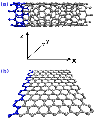
Figure 2: (Color online) Configurations for different systems: (a) Single-walled carbon nanotube; (b) Graphene sheet. The left boundary parts (blue online) are fixed.

In our calculations, the system is relaxed using the Brenner’s potential. Then the dynamical matrix and nonlinear force constants are obtained by finite difference method. The dynamical matrix is diagonalized to obtain the eigen frequencies and eigen vectors. Finally, the eigen frequencies, eigen vectors and nonlinear force constants are used to calculate the GF following the formula in the appendix. Generally, the relevant anharmonic value from Brenner’s potential is about $|k_{lmn}/k_{ij}|\approx 0.8$Å^-1, where $k_{ij}$ is one element in the dynamical matrix.

Fig. 2 is the configurations for SWCNT and graphene in our calculation. For both systems, the smaller balls (blue online) on the left boundaries are fixed atoms while the right boundaries are free. This boundary condition corresponds to thermal expansion under zero pressure. The $x$ axis in SWCNT is along its axial. In graphene, the $x$ axis is along the in-plane horizontal direction, $y$ in the vertical direction and $z$ in the perpendicular direction. Periodic boundary condition is applied in the $y$ direction in graphene.

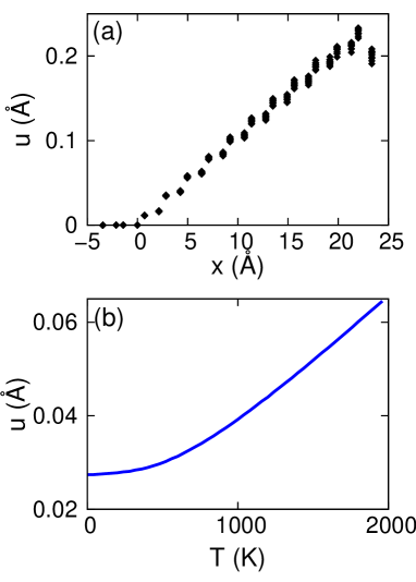
Figure 3: The averaged vibrational displacement $u$ of SWCNT. (a). $u$ v.s. $x$ at $T=1000$ K. (b). $u$ v.s. $T$ for the atom located at $x=3$ Å.

We firstly study the axial thermal expansion in SWCNT. Fig. 3 (a) shows the averaged vibrational displacement in the $x$ direction for different atoms, i.e., $u(x)$. The horizontal axis is the position of each atom along $x$ axis. Generally, $u(x)$ increases with increasing $x$ which reveals the fact that the thermal expansion is homogenous along $x$ axis. On the two boundaries, there are some boundary effects due to the different local environments from atoms in the center region. Fig. 3 (b) shows the temperature dependence for $u$ of one of the atoms in the center region. At high temperatures, $u\propto T$ is the classical behavior. With temperature decreasing, quantum effect appears, and around $T=800$ K, the curve deviates distinctly from the classical behavior. This implies that the Debye temperature in the SWCNT is typically about 800 K. The quantum effect dominates the low temperature region with $T<150$ K. In this temperature region, $u$ keeps a nonzero constant, resulting directly from the combination effect of the thermal zero-point motion and nonlinear interaction in SWCNT. It means that even at $T=0$ K, atoms still vibrate around equilibrium positions, and as a result of the nonlinear interaction, their averaged vibrational displacements is about 1$\%$ of lattice constant from equilibrium positions. This value is not small because the interaction in covalent bonding carbon system is very strong, so the frequencies of the optical phonon modes are high, thus the zero-point motion energy is also high. We expect this temperature dependent curve for $u$ can be confirmed by x-ray or other optical experiments.

Figure 4: (Color online) CTE of SWCNT calculated from the thermal expansion of atoms at different location.

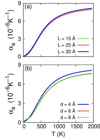
Figure 5: (Color online) Axial CTE v.s. temperature in SWCNT with: (a). diameter $d=4$ Å, and different length $L$; (b). length $L=30$ Å, and different diameter $d$.

The axial CTE ($\alpha_{a}$) of SWCNT can be calculated by using $u_{j}$ of each atom from Eq. (8). Fig. 4 shows the value of axial CTE calculated from different atoms at $T=1000$ K. The horizontal axis is the $x$ position for each atom. SWCNT in this figure is zigzag (5, 0), with length $L=30$ Å. Due to boundary effects on the left and right ends, values for CTE in these two regions deviate obviously from that in the center region. So we drop data on two boundaries and average over other data in the center region to obtain the value of CTE.

Fig. 5 shows the temperature dependence for axial CTE in zigzag SWCNT of different sizes. They are similar to the results of armchair SWCNT. It shows that the length and diameter have small effects on axial CTE, and the value of axial CTE is positive in the whole temperature region. This is consistent with previous results in Ref. LiC, , but different from that in Ref. Jiang, , where the axial CTE depends on diameter sensitively and is negative at low temperature. In general, the value of CTE increases quickly in low temperature region, and reaches the classical limit at high temperatures. We point out that at $T=800$ K, this value still changes a lot with changing temperature. This temperature (800 K) is a bit smaller than the value of Debye temperature in SWCNT or graphene, which is above 1000 K.Benedict ; Tohei ; Falkovsky This result can be understood in the sense that the optical phonon modes play an important role in the calculation of the Debye temperature.Tohei While in the study of the thermal expansion effect, the optical phonon modes are not very important due to their high frequency. So the critical temperature here is lower than Debye temperature.

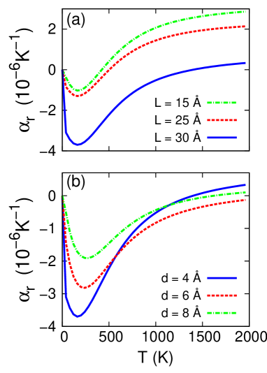
Figure 6: (Color online) Radial CTE of SWCNT with (a). $d=4$ Å and different length; (b). $L=30$ Å and different diameter.

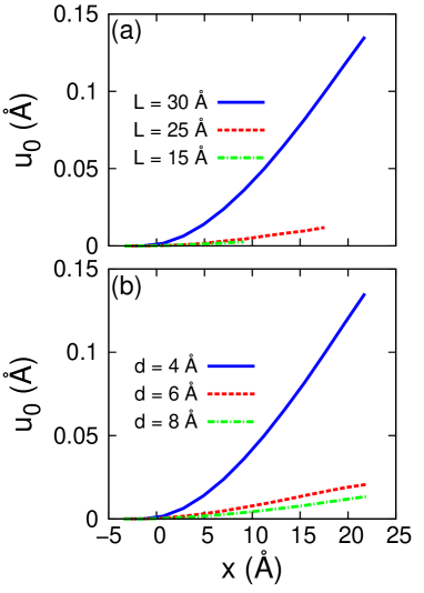
Figure 7: (Color online) The averaged position of axial line at $T=1000$ K in zigzag SWCNT with (a). $d=4$ Å and different length; (b). $L=30$ Å and different diameter.

Fig. 6 is the temperature dependence for the radial CTE ($\alpha_{r}$) of different sized SWCNT. The radial CTE is obtained from the changing of diameter with changing temperature. Compared with the axial CTE, there are abundant behaviors here. (1). Firstly, we can see $\alpha_{r}<0$ in low-temperature region. The origin of this phenomenon is the bending vibration in this rod-like SWCNT system.Krishnan Fig. 7 shows the position for midline in SWCNT along the $x$ axis at $T=1000$ K. This figure indicates the bending vibration directly. This bending vibration has a very low energy thus is very important at low temperatures. It leads to contraction in radial direction in the SWCNT. As a result, the radial CTE is negative in low temperature region where other high energy vibration modes are not excited. (2). A general behavior in both Fig. 6 (a) and (b) is that the thinner SWCNT (with higher aspect ratio length/diameter, $L/d$) has smaller value of $\alpha_{r}$ and larger negative CTE region. This is mainly because the bending vibration in thinner SWCNT is more intense (see Fig. 7). For SWCNT with different diameters shown in Fig. 6 (b), there is one more reason. In SWCNT, another important vibrational mode in the radial direction is the radial breathing mode. This mode can make the SWCNT expand in the radial direction. The frequency of the radial breathing mode is inverse proportional to diameter. So in SWCNT, the larger the diameter, the smaller the frequency of radial breathing mode. Therefore, more positive contribution at low temperatures will lead to larger value of $\alpha_{r}$. The competition between the bending vibration and the radial breathing vibration gives a valley in all curves of $\alpha_{r}$ in Fig. 6. (3). The value of $\alpha_{r}$ is typically one order of magnitude smaller than $\alpha_{a}$. Because along the axial of SWCNT there are some high frequency optical phonon modes, which lead to strong expansion in the axial direction. Another reason is that along the circular direction, SWCNT forms a closed configuration, which makes it more difficult to expand in the radial direction. While in the axial direction, the right side is open and expansion along this direction is easier. In Fig. 6 (a), the CTE does not show convergence behavior with increasing $L$. This is mainly due to very serious bending vibration in long SWCNT. As a result of this strong bending movement, it will be difficult for our method to calculate the radial CTE accurately.

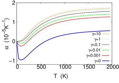
Figure 8: (Color online) CTE v.s. temperature for graphene sheet with various strength of interaction between substrate and graphene. The interaction $\gamma$ is from 0 to 10 eV/(Å${}^{2}u)$.

Now we turn to the thermal expansion in graphene. Graphene is easily bent due to its two-dimensional elastic sheet configuration. So in the experiment it is very difficult to hang a graphene sheet by just holding it on one side (e.g. left side as shown in Fig. 2 (b)). Furthermore, to study the thermal expansion effect, one can not suspend the graphene sheet by fixing both left and right sides. The only reasonable choice is to put the graphene sample on a substrate. In this situation, the substrate can support the graphene stably. But in the mean time, interactions between the substrate and graphene will affect the bending vibration seriously, thus influences the measured value for CTE in graphene sheet. In the following we focus on this substrate effect on the CTE in graphene sheet.

The interaction between substrate and carbon atoms in graphene can be described by the on-site potential in the $z$ directionAizawa : $V=(\gamma/2)u_{z}^{2}$ with $\gamma$ as the interaction force constant in unit of eV/(Ųu). $u_{z}$ is the vibrational displacement in the $z$ direction. Fig. 8 is the CTE of graphene with 204 atoms for different values of $\gamma$. CTE is very sensitive to $\gamma$. When there is no substrate interaction the bending vibration is very strong (which has negative effect on CTE), so the CTE is very small in the high temperature limit, and a large negative CTE region occurs at low temperatures. At $T=300$ K, $\alpha=-6\times 10^{-6}$ K^-1. This value agrees with the very recent experimental result of $-7\times 10^{-6}$ K^-1.BaoW However, when the substrate interaction is introduced, even a very small value of $\gamma=0.001$, can significantly enhance the value of CTE. Furthermore, the negative CTE region considerably shrinks. After further increasing interaction, the value of CTE is further increased; the negative CTE region is further reduced and disappears after $\gamma=0.1$. A saturate value for CTE is obtained after $\gamma=1.0$, where the bending vibration has been suppressed completely by the substrate interaction. We should pointout that the value of $\gamma=0.001$ is actually only about 0.06$\%$ of the interaction between carbon atoms in the two-dimensional graphene sheetSaitoR which is more than 1.67 eV/(Ųu). The practical experimental substrate interaction might be larger than this value. So the measured value of CTE will be higher than the curve with $\gamma=0.001$ in Fig. 8. If the experimental substrate interaction is larger than $\gamma=0.1$, no negative CTE should be observed. By the way, if we compare the saturated value at high temperatures with that in the SWCNT as shown in Fig. 5, we find that the value of CTE in graphene is much larger than SWCNT. This fact implies that the bending vibration in the SWCNT is also very important for the axial CTE. It considerably reduce the value of axial CTE without causing negative axial CTE in SWCNT.

IV conclusion

In conclusion, the GF method has been applied to investigate the CTE in SWCNT and graphene. The effect of quantum zero-point motion and nonlinear interaction at $T=0$ K has been observed clearly. The axial CTE in SWCNT is positive in whole temperature range, while the radial CTE can have negative value at low temperatures. It shows that thinner SWCNT has smaller radial CTE, resulting from the competition between bending vibration and radial breathing vibration. Our calculation displays that the CTE in graphene sheet is very sensitive to the interaction between substrate and graphene, which will greatly enhance the CTE in graphene sheet.

V Acknowledgements

We thank E. Cuansing and Yong Xu for helpful discussions. The work is supported by a Faculty Research Grant of R-144-000-173-101/112 and R-144-000-257-112 of National University of Singapore (NUS), and Grant R-144-000-203-112 from Ministry of Education of Republic of Singapore, and Grant R-144-000-222-646 from NUS.

Appendix A Langreth rules

To arrive at Eq. (7), relations between different types of Green’s functions are in need.WangJS2008 The following Langreth rulesLangreth ; Haug are used to obtain these relations.

For the time invariant contour integral

$$A(\tau,\tau^{\prime})=\int B(\tau,\tau^{\prime\prime})C(\tau^{\prime\prime},\tau^{\prime})d\tau^{\prime\prime},$$ (9)

its Fourier transform has following relations:

$$A^{<}[\omega]=B^{r}[\omega]C^{<}[\omega]+B^{<}[\omega]C^{a}[\omega],$$

$$A^{>}[\omega]=B^{r}[\omega]C^{>}[\omega]+B^{>}[\omega]C^{a}[\omega],$$

$$A^{r}[\omega]=B^{r}[\omega]C^{r}[\omega],$$

$$A^{a}[\omega]=B^{a}[\omega]C^{a}[\omega].$$ (10)

Appendix B Green’s function in eigen space

The retarded GF $G^{r}[\omega]$ can be obtained straightforwardly, since it has the expression asWangJS2008 :

$$G_{0}^{r}[\omega] = [(\omega+i\eta)^{2}I-K]^{-1},$$ (11)

where $K$ is the $N\times N$ force constant matrix, and $\eta$ is a small positive number. $N$ is the degrees of freedom in the system. $I$ is a unit matrix with the same dimension as $K$. As a result,

$$G_{0}^{r}[0] = -K^{-1}.$$ (12)

The calculation of $G^{>}(0)$ is more complicated. However we find that it will be much more advantageous to work in the eigen space.

(a). Firstly, the force constant matrix $K$ is diagonalized:

$$S^{\dagger}KS = \Omega^{2}$$ (13)

where the unitary matrix $S$ stores the information of all eigen vectors. And eigen values are in the diagonalized matrix $\Omega^{2}$:

$$\Omega^{2} = \left(\begin{array}[]{ccccc}\omega_{0}^{2}\\ &\ddots\\ &&\omega_{\mu}^{2}\\ &&&\ddots\\ &&&&\omega_{N-1}^{2}\end{array}\right).$$ (19)

(b). The GF in real space (including both time domain and frequency domain) can be obtained from the corresponding one in the eigen space. We take $G_{0}^{r}[\omega]$ as an example to illustrate this correspondence:

$$G_{0}^{r}[\omega] = [(\omega+i\eta)^{2}I-K]^{-1}$$ (20)

$$= [(\omega+i\eta)^{2}I-S\Omega^{2}S^{\dagger}]^{-1}$$

$$= S[(\omega+i\eta)^{2}I-\Omega^{2}]^{-1}S^{\dagger}$$

$$= SG_{0}^{r}\{\omega\}S^{\dagger},$$

where we have used the relation for two matrices $(AB)^{-1}=B^{-1}A^{-1}$ and we have introduced notation $G_{0}^{r}\{\omega\}=[(\omega+i\eta)^{2}I-\Omega^{2}]^{-1}$ to denote the GF in the eigen space. $G_{0}^{r}\{\omega\}$ is a diagonalized matrix with the element as

$$G_{0}^{r}\{\omega,\omega_{\mu}\} = [(\omega+i\eta)^{2}-\omega_{\mu}^{2}]^{-1}.$$ (21)

Similarly we have,

$$G_{0}^{>}(t)=S\left(G_{0}^{>}\{t\}\right)S^{\dagger}.$$ (22)

This kind of correspondence is valid for other GF, and the relations between different GF in the real space still hold in the eigen space.

(d). From Zeng’s thesisZeng or P. Brouwer’s noteBrouwer , the GF for single oscillator system with frequency $\omega_{0}$ has explicit expression in time domain and frequency domain:

$$G_{0}^{r}(t) = \frac{-i}{2\omega_{0}}\theta(t)\left(e^{-i\omega_{0}t}-e^{i\omega_{0}t}\right),$$ (23)

$$G_{0}^{r}[\omega] = \frac{1}{(\omega+i\eta)^{2}-\omega_{0}^{2}},$$ (24)

$$G_{0}^{a}(t) = \frac{i}{2\omega_{0}}\theta(-t)\left(e^{-i\omega_{0}t}-e^{i\omega_{0}t}\right),$$ (25)

$$G_{0}^{a}[\omega] = \frac{1}{(\omega-i\eta)^{2}-\omega_{0}^{2}},$$ (26)

$$G_{0}^{<}(t) = \frac{-i}{2\omega_{0}}\left[(1+f)e^{i\omega_{0}t}+fe^{-i\omega_{0}t}\right],$$ (27)

$$G_{0}^{<}[\omega] = \frac{-i\pi}{\omega_{0}}\left[\delta(\omega+\omega_{0})(1+f)+\delta(\omega-\omega_{0})f\right],$$ (28)

$$G_{0}^{>}(t) = \frac{-i}{2\omega_{0}}\left[(1+f)e^{-i\omega_{0}t}+fe^{i\omega_{0}t}\right],$$ (29)

$$G_{0}^{>}[\omega] = \frac{-i\pi}{\omega_{0}}\left[\delta(\omega-\omega_{0})(1+f)+\delta(\omega+\omega_{0})f\right],$$ (30)

where $f=f(\omega_{0})=\frac{1}{e^{\beta\hbar\omega_{0}}-1}$ is the Bose distribution function with $\beta=1/(k_{B}T)$.

(e). Using Eq. (22) and  (29), the one point GF $G_{j}$ can be calculated without doing any integration:

$$G_{j} = \sum_{lmn}k_{lmn}G_{lm}^{>}(0)G_{nj}^{r}[0]$$ (33)

$$= \sum_{lmn}k_{lmn}\left(SG_{0}^{>}\{t=0\}S^{\dagger}\right)_{lm}\left(-K^{-1}\right)_{nj}$$

$$= (-i)\sum_{lmn}k_{lmn}\left(S\left(\begin{array}[]{ccc}\ddots\\ &\frac{1}{2\omega_{\mu}}(2f+1)\\ &&\ddots\end{array}\right)S^{\dagger}\right)_{lm}$$

$$\times\left(-K^{-1}\right)_{nj}.$$

In the study of the coefficient of thermal expansion, the derivative of $G_{j}(t)$ with respective to temperature $T$ is needed:

$$\frac{dG_{j}}{dT} = (-i)\sum_{lmn}k_{lmn}\left(S\left(\begin{array}[]{ccc}\ddots\\ &\frac{1}{\omega_{\mu}}(\frac{df}{dT})\\ &&\ddots\end{array}\right)S^{\dagger}\right)_{lm}$$ (36)

$$\times\left(-K^{-1}\right)_{nj}.$$

References

- (1) H. J. Dai, Surf. Sci. 500, 218 (2002).
- (2) M. S. Dresselhaus, G. Dresselhaus, and A. Jorio, Annu. Rev. Mater. Res. 34, 247 (2004).
- (3) K. S. Novoselov and A. K. Geim, Nature Mater. 6, 183 (2007).
- (4) P. Avouris, Z. Chen, and V. Perebeinos, Nat. Nanotechnol. 2, 605 (2007).
- (5) A. H. Castro Neto, F. Guinea, N. M. R. Peres, K. S. Novoselov, and A. K. Geim, Rev. Mod . Phys. 81, 109 (2009).
- (6) A. K. Geim, Science 324, 1530 (2009).
- (7) W. Bao, F. Miao, Z. Chen, H. Zhang, W. Jang, C. Dames, and C. N. Lau, Nat. Nanotechnol. 10, 1038 (2009).
- (8) R. S. Ruoff and D. C. Lorents, Carbon 33, 925 (1995).
- (9) S. Bandow, Jpn. J. Appl. Phys., Part 2 36, L1403 (1997).
- (10) Y. Maniwa, R. Fujiwara, H. Kira, H. Tou, E. Nishibori, M. Takata, M. Sakata, A. Fujiwara, X. Zhao, S. Iijima, and Y. Ando, Phys. Rev. B 64, 073105 (2001).
- (11) Y. Yosida, J. Appl. Phys. 87, 3338 (2000).
- (12) Y. Maniwa, R. Fujiwara, H. Kira, H. Tou, H. Kataura, S. Suzuki, Y. Achiba, E. Nishibori, M. Takata, M. Sakata, A. Fujiwara, and H. Suematsu, Phys. Rev. B 64, 241402(R) (2001).
- (13) A. V. Dolbin, V. B. Eselson, V. G. Gavrilko, V. G. Manzhelii, N. A. Vinnikov, S. N. Popov, and B. Sundqvist, Low Temp. Phys. 34, 678 (2008).
- (14) A. V. Dolbin, V. B. Eselson, V. G. Gavrilko, V. G. Manzhelii, S. N. Popov, N. A. Vinnikov, N. I. Danilenko, and B. Sundqvist, Low Temp. Phys. 35, 484 (2009).
- (15) N. R. Raravikar, P. Keblinski, A. M. Rao, M. S. Dresselhaus, L. S. Schadler, and P. M. Ajayan, Phys. Rev. B 66, 235424 (2002).
- (16) P. K. Schelling and P. Keblinski, Phys. Rev. B 68, 035425 (2003).
- (17) G. Cao, X. Chen, and J. W. Kysar, Phys. Rev. B 72, 235404 (2005).
- (18) Y. K. Kwon, S. Berber, and D. Tomanek, Phys. Rev. Lett. 92, 015901 (2004).
- (19) T. H. K. Barron and M. L. Klein, in Dynamical Properties of Solids, edited by G. K. Horton and A. A. Maradudin (North-Holland, Amsterdam, 1974), Vol. I, p. 391.
- (20) J. Fabian and P. B. Allen, Phys. Rev. Lett. 79, 1885 (1997).
- (21) D. A. Broido, A. Ward, and N. Mingo, Phys. Rev. B 72, 014308 (2005).
- (22) A. Ward, D. A. Broido, D. A. Stewart, and G. Deinzer, Phys. Rev. B 80, 125203 (2009).
- (23) C. Li and T.-W. Chou, Phys. Rev. B 71, 235414 (2005).
- (24) H. Jiang, B. Liu, Y. Huang, and K. C. Hwang, J. Eng. Mater. Technol. 126, 265 (2004).
- (25) N. Mounet and N. Marzari, Phys. Rev. B 71, 205214 (2005).
- (26) N. Bonini, M. Lazzeri, N. Marzari, and F. Mauri, Phys. Rev. Lett. 99, 176802 (2007).
- (27) J.-S. Wang, N. Zeng, J. Wang, and C.K. Gan, Phys. Rev. E 75, 061128 (2007).
- (28) J.-S. Wang, J. Wang, and J. T. Lü, Eur. Phys. J. B, 62, 381 (2008).
- (29) N. Zeng, Ph.D thesis, National Univ. Singapore (2008). At Http://staff.science.nus.edu.sg/~phywjs/NEGF/negf.html.
- (30) D. W. Brenner, O. A. Shenderova, J. A. Harrison, S. J. Stuart, B. Ni, and S. B. Sinnott, J. Phys.:Condens. Matter 14, 783 (2002).
- (31) L. X. Benedict, S. G. Louie and M. L. Cohen, Solid State Commun., 100, 177 (1996).
- (32) T. Tohei, A. Kuwabara, F. Oba, and I. Tanaka, Phys. Rev. B 73, 064304 (2006).
- (33) L. A. Falkovsky, Phys. Rev. B 75, 033409 (2007).
- (34) A. Krishnan, E. Dujardin, T. W. Ebbesen, P. N. Yianilos, and M. M. J. Treacy, Phys. Rev. B 58, 14 013 (1998).
- (35) T. Aizawa, R. Souda,S. Otani, Y. Ishizawa, and C. Oshima, Phys. Rev. B 42, 11469 (1990).
- (36) D. C. Langreth, Linear and non-linear response theory with applications, in Linear and Nonlinear Electron Transport in Solids, edited by J. T. Devreese and V. E. van Doren (Plenum Press, New York and London, 1976).
- (37) H. Haug and A. P. Jauho, Quantum Kinetics in Transport and Optics of Semiconductors, (Springer, New York 1996).
- (38) R. Saito, G. Dresselhaus, and M.S. Dresselhaus, Physical Properties of Carbon Nanotubes (Imperial College Press, London 1998).
- (39) P. Brouwer, Theory of Many-Particle Systems (Lecture notes for P654, Cornell University, Spring 2005).