Cooperative Transmission for a Vector Gaussian Parallel Relay Network

Muryong Kim, , and Sae-Young Chung, 
This work was supported in part by the Center for Broadband OFDM Mobile Access (BrOMA) through the ITRC Program of the Ministry of Information and Communication (MIC), Korea, supervised by the Institute of Information Technology Assessment (IITA). The material in this paper was presented in part at the 45th Annual Allerton Conference on Communication, Control, and Computing, Monticello, IL, September 2007.The authors are with the School of Electrical Engineering and Computer Science, KAIST, Daejeon, Korea (e-mail: muryong@kaist.ac.kr, sychung@ee.kaist.ac.kr).
Abstract

In this paper, we consider a parallel relay network where two relays cooperatively help a source transmit to a destination. We assume the source and the destination nodes are equipped with multiple antennas. Three basic schemes and their achievable rates are studied: Decode-and-Forward (DF), Amplify-and-Forward (AF), and Compress-and-Forward (CF). For the DF scheme, the source transmits two private signals, one for each relay, where dirty paper coding (DPC) is used between the two private streams, and a common signal for both relays. The relays make efficient use of the common information to introduce a proper amount of correlation in the transmission to the destination. We show that the DF scheme achieves the capacity under certain conditions. We also show that the CF scheme is asymptotically optimal in the high relay power limit, regardless of channel ranks. It turns out that the AF scheme also achieves the asymptotic optimality but only when the relays-to-destination channel is full rank. The relative advantages of the three schemes are discussed with numerical results.

Index Terms:
Gaussian parallel relay network, diamond channel, cooperative relaying, common information.

I Introduction

Over the recent years, relaying has been considered as a promising technique that can increase throughput and reliability and enhance the coverage of wireless networks. There have been a number of research results showing different aspects of relay channels. Cover and El Gamal [3] derived the capacity of a class of relay channels with a single relay that helps transmission from a source to a destination. Kramer et al. [4] generalized the results in various ways. Laneman et al. [5] considered cooperative diversity aspects of relay channels. In [23], the authors consider the multiplexing aspects of cooperative communications in multi-antenna relay networks. In [6, 7], multi-antenna relay channels are considered. The use of relays in broadcast scenarios is considered in [4, 8].

In this paper, we study the capacity of a vector Gaussian parallel relay network where two parallel relays help transmission from a source node to a destination node. The network model is first studied by Schein et al. [1], and a set of capacity theorems are derived for the discrete memoryless channel and the scalar Gaussian channel. The authors of [2] considered a similar model but with half-duplex constraint, i.e., relays do not transmit and receive at the same time. Recently, the authors of [22] showed their new achievable rate for general scalar Gaussian relay networks is within a constant number of bits from the cut-set upper bound on the capacity. A new achievable rate for the original Schein’s network is derived using a Combined Amplify-and-Decode Forward (CADF) scheme in [24]. Our network model is different from the earlier ones in that both the broadcast channel (BC) part and the multiple access channel (MAC) part are vector Gaussian channels as the source and the destination nodes are equipped with multiple antennas. As the vector BC is not degraded in general and a simple superposition coding will not suffice. In the vector MAC, correlation between relay signals are not always beneficial, rather, the right amount of correlation may result in a better performance as will be seen in a later section. Throughout the paper, upper bounds and achievable rates by different cooperative transmission strategies: DF, AF and CF are derived.

For the DF scheme, the vector Gaussian parallel relay network can be seen as a cascade of multiple-input single-output (MISO) BC and single-input multiple-output (SIMO) MAC channels. We first extend some earlier results for the discrete memoryless and scalar MACs with common information to the vector Gaussian case, and investigate the characteristics of the three-dimensional achievable rate region. We use a known transmission scheme of [10] for the BC part. Using the BC-MAC schemes, we show that DF achieves the capacity of the vector Gaussian parallel relay network under certain conditions. In addition, we address the importance of common information signaling and correlation control.

We also extend some earlier results for AF and CF to the vector Gaussian case. We show when DF is strictly suboptimal and when AF and CF can outperform DF by comparing the achievable rates and the upper bound. We show that AF is asymptotically optimal in the high relay power limit if the channel rank of the MAC part is full. In addition, we also show that the CF scheme achieves the asymptotic capacity, regardless of the channel ranks.

The rest of the paper is organized as follows. In Section II, we introduce the system model. We derive a capacity upper bound for the vector Gaussian parallel relay network in Section III. Next, we derive achievable rates by the DF, AF and CF schemes in Sections IV, V and VI, respectively. Numerical results and comparison of different schemes are given in Section VII. Conclusions and final remarks are given in Section VIII.

II System Model

The vector Gaussian parallel relay network consists of four nodes: a source, a destination, and two relays. We assume no direct link from the source to the destination. The relays are assumed to be full duplex, i.e., they transmit and receive at the same time. The received signals at the relays and at the destination are given by

yr1subscript𝑦𝑟1\displaystyle y_{r1} =\displaystyle= 𝐠1𝐱s+nr1,subscript𝐠1subscript𝐱𝑠subscript𝑛𝑟1\displaystyle{\bf g}_{1}{\bf x}_{s}+n_{r1},
yr2subscript𝑦𝑟2\displaystyle y_{r2} =\displaystyle= 𝐠2𝐱s+nr2,subscript𝐠2subscript𝐱𝑠subscript𝑛𝑟2\displaystyle{\bf g}_{2}{\bf x}_{s}+n_{r2},
𝐲dsubscript𝐲𝑑\displaystyle{\bf y}_{d} =\displaystyle= 𝐡1xr1+𝐡2xr2+𝐧d,subscript𝐡1subscript𝑥𝑟1subscript𝐡2subscript𝑥𝑟2subscript𝐧𝑑\displaystyle{\bf h}_{1}x_{r1}+{\bf h}_{2}x_{r2}+{\bf n}_{d},

where

  • 𝐱sM×1,xr1,xr2formulae-sequencesubscript𝐱𝑠superscript𝑀1subscript𝑥𝑟1subscript𝑥𝑟2{\bf x}_{s}\in{\mathbb{C}}^{M\times{\rm 1}},x_{r1},x_{r2}\in\mathbb{C} are the transmitted signals from the source and from relays 1 and 2, respectively. Input covariance matrix and power constraint at the source node are given by 𝐐s=𝔼[𝐱s𝐱s]subscript𝐐𝑠𝔼delimited-[]subscript𝐱𝑠superscriptsubscript𝐱𝑠{\bf Q}_{s}={\mathbb{E}}[{{\bf x}_{s}{\bf x}_{s}^{\dagger}}] and tr(𝐐s)Pstrsubscript𝐐𝑠subscript𝑃𝑠{\rm tr}\left({{\bf Q}_{s}}\right)\leq P_{s}, respectively. Power constraints at relays are given by 𝔼[|xr1|2]Pr1𝔼delimited-[]superscriptsubscript𝑥𝑟12subscript𝑃𝑟1{\mathbb{E}}[|x_{r1}|^{2}]\leq P_{r1} and 𝔼[|xr2|2]Pr2𝔼delimited-[]superscriptsubscript𝑥𝑟22subscript𝑃𝑟2{\mathbb{E}}[|x_{r2}|^{2}]\leq P_{r2};

  • yr1,yr2,𝐲dN×1formulae-sequencesubscript𝑦𝑟1subscript𝑦𝑟2subscript𝐲𝑑superscript𝑁1y_{r1},y_{r2}\in\mathbb{C},{\bf y}_{d}\in{\mathbb{C}}^{N\times 1} are the received signals at relays 1 and 2 and at the destination, respectively;

  • 𝐠1,𝐠21×Msubscript𝐠1subscript𝐠2superscript1𝑀{\bf g}_{1},{\bf g}_{2}\in{\mathbb{C}}^{{\rm 1}\times M} are the channel gains from the source to relays 1 and 2, respectively, and 𝐡1,𝐡2N×1subscript𝐡1subscript𝐡2superscript𝑁1{\bf h}_{1},{\bf h}_{2}\in{\mathbb{C}}^{N\times 1} are the channel gains from relays 1 and 2 to the destination, respectively;

  • nr1,nr2,𝐧dN×1formulae-sequencesubscript𝑛𝑟1subscript𝑛𝑟2subscript𝐧𝑑superscript𝑁1n_{r1},n_{r2}\in\mathbb{C},{\bf n}_{d}\in{\mathbb{C}}^{N\times 1} are additive white Gaussian noise (AWGN) at relays 1 and 2 and at the destination, respectively. Noise at the relays and each antenna of the destination node is circularly symmetric complex Gaussian, i.e., nr1,nr2𝒞𝒩(0,1)similar-tosubscript𝑛𝑟1subscript𝑛𝑟2𝒞𝒩01n_{r1},n_{r2}\sim\mathcal{CN}\left({0,1}\right) and 𝐧d𝒞𝒩(0,𝐈)similar-tosubscript𝐧𝑑𝒞𝒩0𝐈{\bf n}_{d}\sim\mathcal{CN}\left(0,\mathbf{I}\right) and they are all independent of each other and from the signals.

Throughout the paper, the following notation will be used,

  • The vector and matrix notations:

    𝐲r=[yr1yr2],𝐱r=[xr1xr2],𝐧r=[nr1nr2],𝐆=[𝐠1𝐠2],𝐇=[𝐡1𝐡2].formulae-sequencesubscript𝐲𝑟delimited-[]subscript𝑦𝑟1missing-subexpressionmissing-subexpressionmissing-subexpressionmissing-subexpressionmissing-subexpressionmissing-subexpressionmissing-subexpressionmissing-subexpressionmissing-subexpressionmissing-subexpressionmissing-subexpressionmissing-subexpressionmissing-subexpressionmissing-subexpressionmissing-subexpressionmissing-subexpressionmissing-subexpressionmissing-subexpressionmissing-subexpressionsubscript𝑦𝑟2missing-subexpressionmissing-subexpressionmissing-subexpressionmissing-subexpressionmissing-subexpressionmissing-subexpressionmissing-subexpressionmissing-subexpressionmissing-subexpressionmissing-subexpressionmissing-subexpressionmissing-subexpressionmissing-subexpressionmissing-subexpressionmissing-subexpressionmissing-subexpressionmissing-subexpressionmissing-subexpressionmissing-subexpressionformulae-sequencesubscript𝐱𝑟delimited-[]subscript𝑥𝑟1missing-subexpressionmissing-subexpressionmissing-subexpressionmissing-subexpressionmissing-subexpressionmissing-subexpressionmissing-subexpressionmissing-subexpressionmissing-subexpressionmissing-subexpressionmissing-subexpressionmissing-subexpressionmissing-subexpressionmissing-subexpressionmissing-subexpressionmissing-subexpressionmissing-subexpressionmissing-subexpressionmissing-subexpressionsubscript𝑥𝑟2missing-subexpressionmissing-subexpressionmissing-subexpressionmissing-subexpressionmissing-subexpressionmissing-subexpressionmissing-subexpressionmissing-subexpressionmissing-subexpressionmissing-subexpressionmissing-subexpressionmissing-subexpressionmissing-subexpressionmissing-subexpressionmissing-subexpressionmissing-subexpressionmissing-subexpressionmissing-subexpressionmissing-subexpressionformulae-sequencesubscript𝐧𝑟delimited-[]subscript𝑛𝑟1missing-subexpressionmissing-subexpressionmissing-subexpressionmissing-subexpressionmissing-subexpressionmissing-subexpressionmissing-subexpressionmissing-subexpressionmissing-subexpressionmissing-subexpressionmissing-subexpressionmissing-subexpressionmissing-subexpressionmissing-subexpressionmissing-subexpressionmissing-subexpressionmissing-subexpressionmissing-subexpressionmissing-subexpressionsubscript𝑛𝑟2missing-subexpressionmissing-subexpressionmissing-subexpressionmissing-subexpressionmissing-subexpressionmissing-subexpressionmissing-subexpressionmissing-subexpressionmissing-subexpressionmissing-subexpressionmissing-subexpressionmissing-subexpressionmissing-subexpressionmissing-subexpressionmissing-subexpressionmissing-subexpressionmissing-subexpressionmissing-subexpressionmissing-subexpressionformulae-sequence𝐆delimited-[]subscript𝐠1missing-subexpressionmissing-subexpressionmissing-subexpressionmissing-subexpressionmissing-subexpressionmissing-subexpressionmissing-subexpressionmissing-subexpressionmissing-subexpressionmissing-subexpressionmissing-subexpressionmissing-subexpressionmissing-subexpressionmissing-subexpressionmissing-subexpressionmissing-subexpressionmissing-subexpressionmissing-subexpressionmissing-subexpressionsubscript𝐠2missing-subexpressionmissing-subexpressionmissing-subexpressionmissing-subexpressionmissing-subexpressionmissing-subexpressionmissing-subexpressionmissing-subexpressionmissing-subexpressionmissing-subexpressionmissing-subexpressionmissing-subexpressionmissing-subexpressionmissing-subexpressionmissing-subexpressionmissing-subexpressionmissing-subexpressionmissing-subexpressionmissing-subexpression𝐇delimited-[]subscript𝐡1subscript𝐡2missing-subexpressionmissing-subexpressionmissing-subexpressionmissing-subexpressionmissing-subexpressionmissing-subexpressionmissing-subexpressionmissing-subexpressionmissing-subexpressionmissing-subexpressionmissing-subexpressionmissing-subexpressionmissing-subexpressionmissing-subexpressionmissing-subexpressionmissing-subexpressionmissing-subexpressionmissing-subexpression\mathbf{y}_{r}=\left[{\begin{array}[]{*{20}c}{y_{r1}}\\ {y_{r2}}\\ \end{array}}\right],\mathbf{x}_{r}=\left[{\begin{array}[]{*{20}c}{x_{r1}}\\ {x_{r2}}\\ \end{array}}\right],\mathbf{n}_{r}=\left[{\begin{array}[]{*{20}c}{n_{r1}}\\ {n_{r2}}\\ \end{array}}\right],\mathbf{G}=\left[{\begin{array}[]{*{20}c}{\mathbf{g}_{1}}\\ {\mathbf{g}_{2}}\\ \end{array}}\right],\mathbf{H}=\left[{\begin{array}[]{*{20}c}{\mathbf{h}_{1}}&{\mathbf{h}_{2}}\\ \end{array}}\right].
  • 𝐱snsuperscriptsubscript𝐱𝑠𝑛{\bf x}_{s}^{n}, xr1nsuperscriptsubscript𝑥𝑟1𝑛x_{r1}^{n}, xr2nsuperscriptsubscript𝑥𝑟2𝑛x_{r2}^{n}, yr1nsuperscriptsubscript𝑦𝑟1𝑛y_{r1}^{n}, yr2nsuperscriptsubscript𝑦𝑟2𝑛y_{r2}^{n}, 𝐲dnsuperscriptsubscript𝐲𝑑𝑛{\bf y}_{d}^{n} denote length-n𝑛n sequences of 𝐱ssubscript𝐱𝑠{\bf x}_{s}, xr1subscript𝑥𝑟1x_{r1}, xr2subscript𝑥𝑟2x_{r2}, yr1subscript𝑦𝑟1y_{r1}, yr2subscript𝑦𝑟2y_{r2}, 𝐲dsubscript𝐲𝑑{\bf y}_{d}, respectively.

  • 𝔼𝐱[]subscript𝔼𝐱delimited-[]\mathbb{E}_{\bf x}[\cdot] denotes expectation with respect to the distribution of 𝐱𝐱\bf x, 𝔼x[|y]\mathbb{E}_{x}[\cdot|y] does expectation with respect to the distribution of x𝑥x conditioned on y𝑦y, and the simpler notation 𝔼[]𝔼delimited-[]\mathbb{E}[\cdot] without subscript will be used as long as it is apparent.

  • ()optsuperscript𝑜𝑝𝑡(\cdot)^{opt} means the optimal value of a variable.

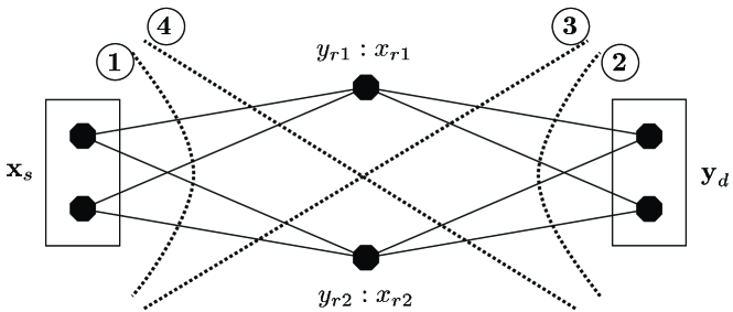
An example for M=N=2𝑀𝑁2M=N=2 case where 𝐇𝐇\mathbf{H} and 𝐆𝐆\mathbf{G} are two-input two-output channels is shown in Fig. 1.

Definition 1

A (2nR,n)superscript2𝑛𝑅𝑛(2^{nR},n) code for vector Gaussian parallel relay network consists of a message set W={1,2,,2nR}𝑊12superscript2𝑛𝑅W=\{1,2,...,2^{nR}\}, an encoding function at the source fs:w{1,2,,2nR}M×n:subscript𝑓𝑠𝑤12superscript2𝑛𝑅superscript𝑀𝑛f_{s}:w\in\{1,2,...,2^{nR}\}\rightarrow\mathbb{C}^{M\times n}, relaying functions at two relays, fr1,i:i1:subscript𝑓𝑟1𝑖superscript𝑖1f_{r1,i}:\mathbb{C}^{i-1}\rightarrow\mathbb{C} and fr2,i:i1:subscript𝑓𝑟2𝑖superscript𝑖1f_{r2,i}:\mathbb{C}^{i-1}\rightarrow\mathbb{C}, respectively, where 1in1𝑖𝑛1\leq i\leq n is the time index111This means that the output of a relay at time i𝑖i depends on all past received symbols. and a decoding function at the destination gd:N×nw^{1,2,,2nR}:subscript𝑔𝑑superscript𝑁𝑛^𝑤12superscript2𝑛𝑅g_{d}:\mathbb{C}^{N\times n}\rightarrow\hat{w}\in\{1,2,...,2^{nR}\}. If the message wW𝑤𝑊w\in W is sent, the conditional probability of error is defined as λ(w)=Pr{gd(𝐲dn)w|w sent}𝜆𝑤Prsubscript𝑔𝑑superscriptsubscript𝐲𝑑𝑛conditional𝑤𝑤 sent\lambda(w)=\Pr\{g_{d}({\bf y}_{d}^{n})\neq w|w\textrm{ sent}\}. The average probability of error is defined as Pe(n)=12nRwλ(w)superscriptsubscript𝑃𝑒𝑛1superscript2𝑛𝑅subscript𝑤𝜆𝑤P_{e}^{(n)}=\frac{1}{2^{nR}}\sum\limits_{w}\lambda(w).

Definition 2

If there exists a sequence of (2nR,n)superscript2𝑛𝑅𝑛(2^{nR},n) codes with Pe(n)0superscriptsubscript𝑃𝑒𝑛0P_{e}^{(n)}\rightarrow 0, the rate R𝑅R is said to be achievable.

Definition 3

The capacity C𝐶C of a vector Gaussian parallel relay network is the supremum of the set of achievable rates.

III Capacity Upper Bound

In this section, we derive the cut-set bound [21] applied to the vector Gaussian parallel relay network. From the four cuts shown in Fig. 2, we get the following cut-set bound:

maxp(𝐱s,xr1,xr2)min[I(𝐱s;yr1,yr2,𝐲d|xr1,xr2),I(xr1,xr2;𝐲d),I(𝐱s,xr1;𝐲d,yr2|xr2),I(𝐱s,xr2;𝐲d,yr1|xr1)].subscript𝑝subscript𝐱𝑠subscript𝑥𝑟1subscript𝑥𝑟2𝐼subscript𝐱𝑠subscript𝑦𝑟1subscript𝑦𝑟2conditionalsubscript𝐲𝑑subscript𝑥𝑟1subscript𝑥𝑟2𝐼subscript𝑥𝑟1subscript𝑥𝑟2subscript𝐲𝑑𝐼subscript𝐱𝑠subscript𝑥𝑟1subscript𝐲𝑑conditionalsubscript𝑦𝑟2subscript𝑥𝑟2𝐼subscript𝐱𝑠subscript𝑥𝑟2subscript𝐲𝑑conditionalsubscript𝑦𝑟1subscript𝑥𝑟1\max\limits_{p(\mathbf{x}_{s},x_{r1},x_{r2})}\min\left[I(\mathbf{x}_{s};y_{r1},y_{r2},\mathbf{y}_{d}|x_{r1},x_{r2}),I(x_{r1},x_{r2};\mathbf{y}_{d}),I(\mathbf{x}_{s},x_{r1};\mathbf{y}_{d},y_{r2}|x_{r2}),I(\mathbf{x}_{s},x_{r2};\mathbf{y}_{d},y_{r1}|x_{r1})\right].

Using the Markovity of the channel, i.e., 𝐱s(xr1,xr2)𝐲dsubscript𝐱𝑠subscript𝑥𝑟1subscript𝑥𝑟2subscript𝐲𝑑\mathbf{x}_{s}\leftrightarrow(x_{r1},x_{r2})\leftrightarrow\mathbf{y}_{d} and (xr1,xr2,𝐲d)𝐱s(yr1,yr2)subscript𝑥𝑟1subscript𝑥𝑟2subscript𝐲𝑑subscript𝐱𝑠subscript𝑦𝑟1subscript𝑦𝑟2(x_{r1},x_{r2},\mathbf{y}_{d})\leftrightarrow\mathbf{x}_{s}\leftrightarrow(y_{r1},y_{r2}), it is easy to get the following loosened cut-set bound:

maxp(𝐱s,xr1,xr2)min[I(𝐱s;yr1,yr2),I(xr1,xr2;𝐲d),I(𝐱s;yr2)+I(xr1;𝐲d|xr2),I(𝐱s;yr1)+I(xr2;𝐲d|xr1)].subscript𝑝subscript𝐱𝑠subscript𝑥𝑟1subscript𝑥𝑟2𝐼subscript𝐱𝑠subscript𝑦𝑟1subscript𝑦𝑟2𝐼subscript𝑥𝑟1subscript𝑥𝑟2subscript𝐲𝑑𝐼subscript𝐱𝑠subscript𝑦𝑟2𝐼subscript𝑥𝑟1conditionalsubscript𝐲𝑑subscript𝑥𝑟2𝐼subscript𝐱𝑠subscript𝑦𝑟1𝐼subscript𝑥𝑟2conditionalsubscript𝐲𝑑subscript𝑥𝑟1\max\limits_{p(\mathbf{x}_{s},x_{r1},x_{r2})}\min\left[I(\mathbf{x}_{s};y_{r1},y_{r2}),I(x_{r1},x_{r2};\mathbf{y}_{d}),I(\mathbf{x}_{s};y_{r2})+I(x_{r1};\mathbf{y}_{d}|x_{r2}),I(\mathbf{x}_{s};y_{r1})+I(x_{r2};\mathbf{y}_{d}|x_{r1})\right].

For example, for the first term we get

I(𝐱s;yr1,yr2,𝐲d|xr1,xr2)𝐼subscript𝐱𝑠subscript𝑦𝑟1subscript𝑦𝑟2conditionalsubscript𝐲𝑑subscript𝑥𝑟1subscript𝑥𝑟2\displaystyle I(\mathbf{x}_{s};y_{r1},y_{r2},\mathbf{y}_{d}|x_{r1},x_{r2}) =I(𝐱s;yr1,yr2|xr1,xr2)+I(𝐱s;𝐲d|xr1,xr2,yr1,yr2)absent𝐼subscript𝐱𝑠subscript𝑦𝑟1conditionalsubscript𝑦𝑟2subscript𝑥𝑟1subscript𝑥𝑟2𝐼subscript𝐱𝑠conditionalsubscript𝐲𝑑subscript𝑥𝑟1subscript𝑥𝑟2subscript𝑦𝑟1subscript𝑦𝑟2\displaystyle=I(\mathbf{x}_{s};y_{r1},y_{r2}|x_{r1},x_{r2})+I(\mathbf{x}_{s};\mathbf{y}_{d}|x_{r1},x_{r2},y_{r1},y_{r2})
I(𝐱s;yr1,yr2)+I(𝐱s;𝐲d|xr1,xr2,yr1,yr2)absent𝐼subscript𝐱𝑠subscript𝑦𝑟1subscript𝑦𝑟2𝐼subscript𝐱𝑠conditionalsubscript𝐲𝑑subscript𝑥𝑟1subscript𝑥𝑟2subscript𝑦𝑟1subscript𝑦𝑟2\displaystyle\leq I(\mathbf{x}_{s};y_{r1},y_{r2})+I(\mathbf{x}_{s};\mathbf{y}_{d}|x_{r1},x_{r2},y_{r1},y_{r2})
=I(𝐱s;yr1,yr2)absent𝐼subscript𝐱𝑠subscript𝑦𝑟1subscript𝑦𝑟2\displaystyle=I(\mathbf{x}_{s};y_{r1},y_{r2})

where the inequality and the last equality follows from the Markovity (xr1,xr2,𝐲d)𝐱s(yr1,yr2)subscript𝑥𝑟1subscript𝑥𝑟2subscript𝐲𝑑subscript𝐱𝑠subscript𝑦𝑟1subscript𝑦𝑟2(x_{r1},x_{r2},\mathbf{y}_{d})\leftrightarrow\mathbf{x}_{s}\leftrightarrow(y_{r1},y_{r2}). For the third term we get

I(𝐱s,xr1;𝐲d,yr2|xr2)𝐼subscript𝐱𝑠subscript𝑥𝑟1subscript𝐲𝑑conditionalsubscript𝑦𝑟2subscript𝑥𝑟2\displaystyle I(\mathbf{x}_{s},x_{r1};\mathbf{y}_{d},y_{r2}|x_{r2}) =I(𝐱s,xr1;𝐲d|xr2)+I(𝐱s,xr1;yr2|xr2,𝐲d)absent𝐼subscript𝐱𝑠subscript𝑥𝑟1conditionalsubscript𝐲𝑑subscript𝑥𝑟2𝐼subscript𝐱𝑠subscript𝑥𝑟1conditionalsubscript𝑦𝑟2subscript𝑥𝑟2subscript𝐲𝑑\displaystyle=I(\mathbf{x}_{s},x_{r1};\mathbf{y}_{d}|x_{r2})+I(\mathbf{x}_{s},x_{r1};y_{r2}|x_{r2},\mathbf{y}_{d})
=I(xr1;𝐲d|xr2)+I(𝐱s;𝐲d|xr1,xr2)+I(𝐱s,xr1;yr2|xr2,𝐲d)absent𝐼subscript𝑥𝑟1conditionalsubscript𝐲𝑑subscript𝑥𝑟2𝐼subscript𝐱𝑠conditionalsubscript𝐲𝑑subscript𝑥𝑟1subscript𝑥𝑟2𝐼subscript𝐱𝑠subscript𝑥𝑟1conditionalsubscript𝑦𝑟2subscript𝑥𝑟2subscript𝐲𝑑\displaystyle=I(x_{r1};\mathbf{y}_{d}|x_{r2})+I(\mathbf{x}_{s};\mathbf{y}_{d}|x_{r1},x_{r2})+I(\mathbf{x}_{s},x_{r1};y_{r2}|x_{r2},\mathbf{y}_{d})
=I(xr1;𝐲d|xr2)+I(𝐱s,xr1;yr2|xr2,𝐲d)absent𝐼subscript𝑥𝑟1conditionalsubscript𝐲𝑑subscript𝑥𝑟2𝐼subscript𝐱𝑠subscript𝑥𝑟1conditionalsubscript𝑦𝑟2subscript𝑥𝑟2subscript𝐲𝑑\displaystyle=I(x_{r1};\mathbf{y}_{d}|x_{r2})+I(\mathbf{x}_{s},x_{r1};y_{r2}|x_{r2},\mathbf{y}_{d})
=I(xr1;𝐲d|xr2)+I(𝐱s;yr2|xr2,𝐲d)+I(xr1;yr2|𝐱s,xr2,𝐲d)absent𝐼subscript𝑥𝑟1conditionalsubscript𝐲𝑑subscript𝑥𝑟2𝐼subscript𝐱𝑠conditionalsubscript𝑦𝑟2subscript𝑥𝑟2subscript𝐲𝑑𝐼subscript𝑥𝑟1conditionalsubscript𝑦𝑟2subscript𝐱𝑠subscript𝑥𝑟2subscript𝐲𝑑\displaystyle=I(x_{r1};\mathbf{y}_{d}|x_{r2})+I(\mathbf{x}_{s};y_{r2}|x_{r2},\mathbf{y}_{d})+I(x_{r1};y_{r2}|\mathbf{x}_{s},x_{r2},\mathbf{y}_{d})
=I(xr1;𝐲d|xr2)+I(𝐱s;yr2|xr2,𝐲d)absent𝐼subscript𝑥𝑟1conditionalsubscript𝐲𝑑subscript𝑥𝑟2𝐼subscript𝐱𝑠conditionalsubscript𝑦𝑟2subscript𝑥𝑟2subscript𝐲𝑑\displaystyle=I(x_{r1};\mathbf{y}_{d}|x_{r2})+I(\mathbf{x}_{s};y_{r2}|x_{r2},\mathbf{y}_{d})
I(xr1;𝐲d|xr2)+I(𝐱s;yr2)absent𝐼subscript𝑥𝑟1conditionalsubscript𝐲𝑑subscript𝑥𝑟2𝐼subscript𝐱𝑠subscript𝑦𝑟2\displaystyle\leq I(x_{r1};\mathbf{y}_{d}|x_{r2})+I(\mathbf{x}_{s};y_{r2})

where the third equality follows from the Markovity 𝐱s(xr1,xr2)𝐲dsubscript𝐱𝑠subscript𝑥𝑟1subscript𝑥𝑟2subscript𝐲𝑑\mathbf{x}_{s}\leftrightarrow(x_{r1},x_{r2})\leftrightarrow\mathbf{y}_{d} and the fifth equality and the inequality follow from the Markovity (xr1,xr2,𝐲d)𝐱s(yr1,yr2)subscript𝑥𝑟1subscript𝑥𝑟2subscript𝐲𝑑subscript𝐱𝑠subscript𝑦𝑟1subscript𝑦𝑟2(x_{r1},x_{r2},\mathbf{y}_{d})\leftrightarrow\mathbf{x}_{s}\leftrightarrow(y_{r1},y_{r2}).

Note that this cut-set bound is optimized over the joint input distribution p(𝐱s,xr1,xr2)𝑝subscript𝐱𝑠subscript𝑥𝑟1subscript𝑥𝑟2p(\mathbf{x}_{s},x_{r1},x_{r2}). Using this, we get the following capacity upper bound for the vector Gaussian parallel relay network.

Theorem 1

The capacity of the vector Gaussian parallel relay network is upper bounded by the minimum of the three expressions given by

CRsum,BCupper=max𝐐s,tr(𝐐s)Pslogdet(𝐈+𝐆𝐐s𝐆),𝐶superscriptsubscript𝑅𝑠𝑢𝑚𝐵𝐶𝑢𝑝𝑝𝑒𝑟subscriptsubscript𝐐𝑠trsubscript𝐐𝑠subscript𝑃𝑠𝐈subscript𝐆𝐐𝑠superscript𝐆\displaystyle C\leq R_{sum,BC}^{upper}=\mathop{\max}\limits_{\mathbf{Q}_{s},\operatorname{tr}(\mathbf{Q}_{s})\leq P_{s}}\log\det\left({\mathbf{I}+\mathbf{GQ}_{s}\mathbf{G}^{\dagger}}\right), (1)
Cmax|ρ|[0,1]min[logdet(𝐈+𝐇𝐐r𝐇),log[(1+Ps𝐠22)(1+(1|ρ|2)Pr1𝐡12)]],𝐶subscript𝜌01𝐈subscript𝐇𝐐𝑟superscript𝐇1subscript𝑃𝑠superscriptnormsubscript𝐠2211superscript𝜌2subscript𝑃𝑟1superscriptnormsubscript𝐡12\displaystyle C\leq\mathop{\max}\limits_{|\rho|\in[0,1]}\min\left[{\log\det\left({\mathbf{I}+\mathbf{HQ}_{r}\mathbf{H}^{\dagger}}\right),\log[({1+P_{s}\left\|{\mathbf{g}_{2}}\right\|^{2}})({1+(1-|\rho|^{2})P_{r1}\left\|{\mathbf{h}_{1}}\right\|^{2}})]}\right], (2)
Cmax|ρ|[0,1]min[logdet(𝐈+𝐇𝐐r𝐇),log[(1+Ps𝐠12)(1+(1|ρ|2)Pr2𝐡22)]].𝐶subscript𝜌01𝐈subscript𝐇𝐐𝑟superscript𝐇1subscript𝑃𝑠superscriptnormsubscript𝐠1211superscript𝜌2subscript𝑃𝑟2superscriptnormsubscript𝐡22\displaystyle C\leq\mathop{\max}\limits_{|\rho|\in[0,1]}\min\left[{\log\det\left({\mathbf{I}+\mathbf{HQ}_{r}\mathbf{H}^{\dagger}}\right),\log[({1+P_{s}\left\|{\mathbf{g}_{1}}\right\|^{2}})(1+(1-|\rho|^{2})P_{r2}\left\|{\mathbf{h}_{2}}\right\|^{2})]}\right]. (3)

where 𝐐r=𝔼[𝐱r𝐱r]=[Pr1|ρ|ej𝐡1𝐡2Pr1Pr2|ρ|ej𝐡1𝐡2Pr1Pr2Pr2]subscript𝐐𝑟𝔼delimited-[]subscript𝐱𝑟superscriptsubscript𝐱𝑟delimited-[]subscript𝑃𝑟1𝜌superscript𝑒𝑗superscriptsubscript𝐡1subscript𝐡2subscript𝑃𝑟1subscript𝑃𝑟2missing-subexpressionmissing-subexpressionmissing-subexpressionmissing-subexpressionmissing-subexpressionmissing-subexpressionmissing-subexpressionmissing-subexpressionmissing-subexpressionmissing-subexpressionmissing-subexpressionmissing-subexpressionmissing-subexpressionmissing-subexpressionmissing-subexpressionmissing-subexpressionmissing-subexpressionmissing-subexpression𝜌superscript𝑒𝑗superscriptsubscript𝐡1subscript𝐡2subscript𝑃𝑟1subscript𝑃𝑟2subscript𝑃𝑟2missing-subexpressionmissing-subexpressionmissing-subexpressionmissing-subexpressionmissing-subexpressionmissing-subexpressionmissing-subexpressionmissing-subexpressionmissing-subexpressionmissing-subexpressionmissing-subexpressionmissing-subexpressionmissing-subexpressionmissing-subexpressionmissing-subexpressionmissing-subexpressionmissing-subexpressionmissing-subexpression\mathbf{Q}_{r}=\mathbb{E}[\mathbf{x}_{r}\mathbf{x}_{r}^{\dagger}]=\left[{\begin{array}[]{*{20}c}{P_{r1}}&{|\rho|e^{j\angle\mathbf{h}_{1}^{\dagger}\mathbf{h}_{2}}{\sqrt{P_{r1}P_{r2}}}}\\ {|\rho|e^{-j\angle\mathbf{h}_{1}^{\dagger}\mathbf{h}_{2}}{\sqrt{P_{r1}P_{r2}}}}&{P_{r2}}\\ \end{array}}\right].

Proof:

From the first cut, the following upper bound is derived:

I(𝐱s;yr1,yr2)𝐼subscript𝐱𝑠subscript𝑦𝑟1subscript𝑦𝑟2\displaystyle I(\mathbf{x}_{s};y_{r1},y_{r2}) =\displaystyle= h(yr1,yr2)h(yr1,yr2|𝐱s)subscript𝑦𝑟1subscript𝑦𝑟2subscript𝑦𝑟1conditionalsubscript𝑦𝑟2subscript𝐱𝑠\displaystyle h(y_{r1},y_{r2})-h(y_{r1},y_{r2}|\mathbf{x}_{s})
=\displaystyle= h(𝐲r)h(𝐧r)subscript𝐲𝑟subscript𝐧𝑟\displaystyle h(\mathbf{y}_{r})-h(\mathbf{n}_{r})
\displaystyle\leq log(2πe)2det𝔼[𝐲r𝐲r]log(2πe)2det𝔼[𝐧r𝐧r]\displaystyle\log(2\pi e)^{2}\det\mathbb{E}[\mathbf{y}_{r}\mathbf{y}_{r}^{{\dagger}}]-\log(2\pi e)^{2}\det\mathbb{E}[\mathbf{n}_{r}\mathbf{n}_{r}^{{\dagger}}]
=\displaystyle= logdet𝔼[𝐧r𝐧r+𝐆𝐱s𝐱s𝐆]𝔼delimited-[]subscript𝐧𝑟superscriptsubscript𝐧𝑟subscript𝐆𝐱𝑠superscriptsubscript𝐱𝑠superscript𝐆\displaystyle\log\det\mathbb{E}[\mathbf{n}_{r}\mathbf{n}_{r}^{{\dagger}}+\mathbf{Gx}_{s}\mathbf{x}_{s}^{{\dagger}}\mathbf{G}^{{\dagger}}]
=\displaystyle= logdet(𝐈+𝐆𝐐s𝐆)𝐈subscript𝐆𝐐𝑠superscript𝐆\displaystyle\log\det(\mathbf{I+GQ}_{s}\mathbf{G}^{{\dagger}})

where the inequality follows from the fact that the circularly symmetric complex Gaussian maximizes the entropy [19]. From the second cut, the following upper bound is derived:

I(xr1,xr2;𝐲d)𝐼subscript𝑥𝑟1subscript𝑥𝑟2subscript𝐲𝑑\displaystyle I(x_{r1},x_{r2};\mathbf{y}_{d}) =\displaystyle= h(𝐲d)h(𝐲d|xr1,xr2)subscript𝐲𝑑conditionalsubscript𝐲𝑑subscript𝑥𝑟1subscript𝑥𝑟2\displaystyle h(\mathbf{y}_{d})-h(\mathbf{y}_{d}|x_{r1},x_{r2})
=\displaystyle= h(𝐲d)h(𝐧d)subscript𝐲𝑑subscript𝐧𝑑\displaystyle h(\mathbf{y}_{d})-h(\mathbf{n}_{d})
\displaystyle\leq log(2πe)Ndet𝔼[𝐲d𝐲d]log(2πe)Ndet𝔼[𝐧d𝐧d]\displaystyle\log(2\pi e)^{N}\det\mathbb{E}[\mathbf{y}_{d}\mathbf{y}_{d}^{\mathbf{{\dagger}}}]-\log(2\pi e)^{N}\det\mathbb{E}[\mathbf{n}_{d}\mathbf{n}_{d}^{\mathbf{{\dagger}}}]
=\displaystyle= logdet𝔼[𝐧d𝐧d+𝐡1𝐡1|xr1|2+𝐡2𝐡2|xr2|2+𝐡1𝐡2xr1xr2+𝐡2𝐡1xr1xr2]𝔼delimited-[]subscript𝐧𝑑superscriptsubscript𝐧𝑑subscript𝐡1superscriptsubscript𝐡1superscriptsubscript𝑥𝑟12subscript𝐡2superscriptsubscript𝐡2superscriptsubscript𝑥𝑟22subscript𝐡1superscriptsubscript𝐡2subscript𝑥𝑟1superscriptsubscript𝑥𝑟2subscript𝐡2superscriptsubscript𝐡1superscriptsubscript𝑥𝑟1subscript𝑥𝑟2\displaystyle\log\det\mathbb{E}[\mathbf{n}_{d}\mathbf{n}_{d}^{\mathbf{{\dagger}}}+\mathbf{h}_{1}\mathbf{h}_{1}^{\mathbf{{\dagger}}}|x_{r1}|^{2}+\mathbf{h}_{2}\mathbf{h}_{2}^{\mathbf{{\dagger}}}|x_{r2}|^{2}+\mathbf{h}_{1}\mathbf{h}_{2}^{\mathbf{{\dagger}}}x_{r1}x_{r2}^{*}+\mathbf{h}_{2}\mathbf{h}_{1}^{\mathbf{{\dagger}}}x_{r1}^{*}x_{r2}]
=\displaystyle= logdet(𝐈+𝐡𝟏𝐡𝟏Pr1+𝐡2𝐡2Pr2+𝐡1𝐡2ρPr1Pr2+𝐡2𝐡1ρPr1Pr2)𝐈subscript𝐡1superscriptsubscript𝐡1subscript𝑃𝑟1subscript𝐡2superscriptsubscript𝐡2subscript𝑃𝑟2subscript𝐡1superscriptsubscript𝐡2𝜌subscript𝑃𝑟1subscript𝑃𝑟2subscript𝐡2superscriptsubscript𝐡1superscript𝜌subscript𝑃𝑟1subscript𝑃𝑟2\displaystyle\log\det(\mathbf{I}+\mathbf{h}_{\mathbf{1}}\mathbf{h}_{\mathbf{1}}^{\mathbf{{\dagger}}}P_{r1}+\mathbf{h}_{2}\mathbf{h}_{2}^{\mathbf{{\dagger}}}P_{r2}+\mathbf{h}_{1}\mathbf{h}_{2}^{\mathbf{{\dagger}}}\rho\sqrt{P_{r1}P_{r2}}+\mathbf{h}_{2}\mathbf{h}_{1}^{\mathbf{{\dagger}}}\rho^{*}\sqrt{P_{r1}P_{r2}})
=\displaystyle= logdet(𝐈+𝐇𝐐r𝐇).𝐈subscript𝐇𝐐𝑟superscript𝐇\displaystyle\log\det(\mathbf{I}+\mathbf{HQ}_{r}\mathbf{H}^{\mathbf{{\dagger}}}).

where ρ=𝔼[xr1xr2]Pr1Pr2𝜌𝔼delimited-[]subscript𝑥𝑟1superscriptsubscript𝑥𝑟2subscript𝑃𝑟1subscript𝑃𝑟2\rho=\frac{{\mathbb{E}[x_{r1}x_{r2}^{*}]}}{{\sqrt{P_{r1}P_{r2}}}} and note that we set ρ=𝐡1𝐡2𝜌superscriptsubscript𝐡1subscript𝐡2\angle\rho=\angle\mathbf{h}_{1}^{\dagger}\mathbf{h}_{2} in (2) and (3). From the third cut, the following upper bounds are derived:

I(𝐱s;yr2)+I(xr1;𝐲d|xr2)𝐼subscript𝐱𝑠subscript𝑦𝑟2𝐼subscript𝑥𝑟1conditionalsubscript𝐲𝑑subscript𝑥𝑟2\displaystyle I(\mathbf{x}_{s};y_{r2})+I(x_{r1};\mathbf{y}_{d}|x_{r2}) \displaystyle\leq log(1+𝐠2𝐐s𝐠2)+log(1+(1|ρ|2)Pr1𝐡12)1subscript𝐠2subscript𝐐𝑠superscriptsubscript𝐠211superscript𝜌2subscript𝑃𝑟1superscriptnormsubscript𝐡12\displaystyle\log(1+\mathbf{g}_{2}\mathbf{Q}_{s}\mathbf{g}_{2}^{\dagger})+\log(1+(1-|\rho|^{2})P_{r1}\left\|{\mathbf{h}_{1}}\right\|^{2})
\displaystyle\leq log(1+Ps𝐠22)+log(1+(1|ρ|2)Pr1𝐡12)1subscript𝑃𝑠superscriptnormsubscript𝐠2211superscript𝜌2subscript𝑃𝑟1superscriptnormsubscript𝐡12\displaystyle\log(1+P_{s}\left\|{\mathbf{g}_{2}}\right\|^{2})+\log(1+(1-|\rho|^{2})P_{r1}\left\|{\mathbf{h}_{1}}\right\|^{2})

where the first inequality follows from the fact that the circularly symmetric complex Gaussian distribution maximized differential entropy and from the following property:

𝔼xr2[𝔼xr1{|xr1|2|xr2}|𝔼xr1{xr1|xr2}|2](1|ρ|2)Pr1,subscript𝔼subscript𝑥𝑟2delimited-[]subscript𝔼subscript𝑥𝑟1conditionalsuperscriptsubscript𝑥𝑟12subscript𝑥𝑟2superscriptsubscript𝔼subscript𝑥𝑟1conditional-setsubscript𝑥𝑟1subscript𝑥𝑟221superscript𝜌2subscript𝑃𝑟1\mathbb{E}_{x_{r2}}\left[\mathbb{E}_{x_{r1}}\{\left|{x_{r1}}\right|^{2}|x_{r2}\}-\left|\mathbb{E}_{x_{r1}}\{x_{r1}|x_{r2}\}\right|^{2}\right]\leq(1-|\rho|^{2})P_{r1},

and for the second inequality 𝐐s=Ps𝐠22𝐠2𝐠2subscript𝐐𝑠subscript𝑃𝑠superscriptnormsubscript𝐠22superscriptsubscript𝐠2subscript𝐠2\mathbf{Q}_{s}=\frac{{P_{s}}}{{\left\|\mathbf{g}_{2}\right\|^{2}}}{\mathbf{g}_{2}^{\dagger}\mathbf{g}_{2}} is used. Similarly, from the fourth cut:

I(𝐱s;yr1)+I(xr2;𝐲d|xr1)𝐼subscript𝐱𝑠subscript𝑦𝑟1𝐼subscript𝑥𝑟2conditionalsubscript𝐲𝑑subscript𝑥𝑟1\displaystyle I(\mathbf{x}_{s};y_{r1})+I(x_{r2};\mathbf{y}_{d}|x_{r1}) \displaystyle\leq log(1+𝐠1𝐐s𝐠1)+log(1+(1|ρ|2)Pr2𝐡22)1subscript𝐠1subscript𝐐𝑠superscriptsubscript𝐠111superscript𝜌2subscript𝑃𝑟2superscriptnormsubscript𝐡22\displaystyle\log(1+\mathbf{g}_{1}\mathbf{Q}_{s}\mathbf{g}_{1}^{\dagger})+\log(1+(1-|\rho|^{2})P_{r2}\left\|{\mathbf{h}_{2}}\right\|^{2})
\displaystyle\leq log(1+Ps𝐠12)+log(1+(1|ρ|2)Pr2𝐡22).1subscript𝑃𝑠superscriptnormsubscript𝐠1211superscript𝜌2subscript𝑃𝑟2superscriptnormsubscript𝐡22\displaystyle\log(1+P_{s}\left\|\mathbf{g}_{1}\right\|^{2})+\log(1+(1-|\rho|^{2})P_{r2}\left\|{\mathbf{h}_{2}}\right\|^{2}).

By properly combining the above four bounds, we can see that the minimum of the three expressions given in the theorem statement results in a tighter upper bound. ∎

IV Decode-and-Forward (DF)

In this section, we describe an achievable rate of the vector Gaussian parallel relay network with a DF strategy. With DF, the signal is delivered from the source to the destination in a two hop transmission. The source has three message sets: m1{1,2,,2nR1}subscript𝑚112superscript2𝑛subscript𝑅1m_{1}\in\{1,2,...,2^{nR_{1}}\} intended for relay 1, m2{1,2,,2nR2}subscript𝑚212superscript2𝑛subscript𝑅2m_{2}\in\{1,2,...,2^{nR_{2}}\} for relay 2, and mc{1,2,,2nRc}subscript𝑚𝑐12superscript2𝑛subscript𝑅𝑐m_{c}\in\{1,2,...,2^{nR_{c}}\} for both relays. Depending on the messages to transmit, the source node makes the signal 𝐱ssubscript𝐱𝑠\mathbf{x}_{s} as a function of m1subscript𝑚1m_{1}, m2subscript𝑚2m_{2} and mcsubscript𝑚𝑐m_{c}. Upon successful decoding of the signals, relays know their private messages and the common message. The relays re-encode the received information to make input signals xr1subscript𝑥𝑟1x_{r1} as a function of m1subscript𝑚1m_{1} and mcsubscript𝑚𝑐m_{c}, and xr2subscript𝑥𝑟2x_{r2} as a function of m2subscript𝑚2m_{2} and mcsubscript𝑚𝑐m_{c} as a block Markov manner. As the end-to-end channel is a cascade of MISO BC and SIMO MAC both with common information, we first investigate optimal signaling in the second hop.

IV-A The Second Hop: SIMO MAC with Common Information

The capacity region of the discrete memoryless MAC with common information is derived in [14, 16] and that of scalar Gaussian MAC with common information in [17]. The characteristics of the scalar Gaussian MAC were further investigated in [18]. The result can be extended to the Gaussian MAC with multiple antennas at the destination.

Definition 4

A ((2nR1×2nRc,2nR2×2nRc),n)superscript2𝑛subscript𝑅1superscript2𝑛subscript𝑅𝑐superscript2𝑛subscript𝑅2superscript2𝑛subscript𝑅𝑐𝑛((2^{nR_{1}}\times 2^{nR_{c}},2^{nR_{2}}\times 2^{nR_{c}}),n) code for the SIMO MAC with common information consists of three message sets m1={1,2,,2nR1}subscript𝑚112superscript2𝑛subscript𝑅1m_{1}=\{1,2,...,2^{nR_{1}}\}, m2={1,2,,2nR2}subscript𝑚212superscript2𝑛subscript𝑅2m_{2}=\{1,2,...,2^{nR_{2}}\}, mc={1,2,,2nRc}subscript𝑚𝑐12superscript2𝑛subscript𝑅𝑐m_{c}=\{1,2,...,2^{nR_{c}}\}, encoding functions at two relays, fr1:(m1,mc)n:subscript𝑓𝑟1subscript𝑚1subscript𝑚𝑐superscript𝑛f_{r1}:(m_{1},m_{c})\rightarrow\mathbb{C}^{n} and fr2:(m2,mc)n:subscript𝑓𝑟2subscript𝑚2subscript𝑚𝑐superscript𝑛f_{r2}:(m_{2},m_{c})\rightarrow\mathbb{C}^{n}, respectively, and a decoding function at the destination gd:M×n(m^1,m^2,m^c):subscript𝑔𝑑superscript𝑀𝑛subscript^𝑚1subscript^𝑚2subscript^𝑚𝑐g_{d}:\mathbb{C}^{M\times n}\rightarrow(\hat{m}_{1},\hat{m}_{2},\hat{m}_{c}). If the messages (m1,m2,mc)subscript𝑚1subscript𝑚2subscript𝑚𝑐(m_{1},m_{2},m_{c}) are sent, the conditional probability of error is λ(m1,m2,mc)=Pr{gd(𝐲dn)(m1,m2,mc)|(m1,m2,mc) sent}𝜆subscript𝑚1subscript𝑚2subscript𝑚𝑐Prsubscript𝑔𝑑superscriptsubscript𝐲𝑑𝑛conditionalsubscript𝑚1subscript𝑚2subscript𝑚𝑐subscript𝑚1subscript𝑚2subscript𝑚𝑐 sent\lambda(m_{1},m_{2},m_{c})=\Pr\{g_{d}({\bf y}_{d}^{n})\neq(m_{1},m_{2},m_{c})|(m_{1},m_{2},m_{c})\textrm{ sent}\}. The average probability of error is defined as Pe(n)=12n(R1+R2+Rc)(m1,m2,mc)λ(m1,m2,mc)superscriptsubscript𝑃𝑒𝑛1superscript2𝑛subscript𝑅1subscript𝑅2subscript𝑅𝑐subscriptsubscript𝑚1subscript𝑚2subscript𝑚𝑐𝜆subscript𝑚1subscript𝑚2subscript𝑚𝑐P_{e}^{(n)}=\frac{1}{2^{n(R_{1}+R_{2}+R_{c})}}\sum\limits_{(m_{1},m_{2},m_{c})}\lambda(m_{1},m_{2},m_{c}).

Definition 5

If there exists a sequence of ((2nR1×2nRc,2nR2×2nRc),n)superscript2𝑛subscript𝑅1superscript2𝑛subscript𝑅𝑐superscript2𝑛subscript𝑅2superscript2𝑛subscript𝑅𝑐𝑛((2^{nR_{1}}\times 2^{nR_{c}},2^{nR_{2}}\times 2^{nR_{c}}),n) codes with Pe(n)0superscriptsubscript𝑃𝑒𝑛0P_{e}^{(n)}\rightarrow 0, the rate triplet (R1,R2,Rc)subscript𝑅1subscript𝑅2subscript𝑅𝑐(R_{1},R_{2},R_{c}) is said to be achievable.

Definition 6

The capacity region of the SIMO MAC with common information is the closure of the set of all achievable rate triplets.

We will derive an achievable rate region assuming Gaussian input distributions. Each relay’s input signal is a superposition of private and common signals:

xr1n(m1,mc)=vn(m1)+αPr1Pcu1n(mc),xr2n(m2,mc)=wn(m2)+βPr2Pcu2n(mc)formulae-sequencesuperscriptsubscript𝑥𝑟1𝑛subscript𝑚1subscript𝑚𝑐superscript𝑣𝑛subscript𝑚1𝛼subscript𝑃𝑟1subscript𝑃𝑐superscriptsubscript𝑢1𝑛subscript𝑚𝑐superscriptsubscript𝑥𝑟2𝑛subscript𝑚2subscript𝑚𝑐superscript𝑤𝑛subscript𝑚2𝛽subscript𝑃𝑟2subscript𝑃𝑐superscriptsubscript𝑢2𝑛subscript𝑚𝑐x_{r1}^{n}(m_{1},m_{c})=v^{n}(m_{1})+\sqrt{\frac{{\alpha P_{r1}}}{{P_{c}}}}u_{1}^{n}(m_{c}),\ \ \ \ \ \ x_{r2}^{n}(m_{2},m_{c})=w^{n}(m_{2})+\sqrt{\frac{{\beta P_{r2}}}{{P_{c}}}}u_{2}^{n}(m_{c})

where v𝒞𝒩(0,α¯Pr1)similar-to𝑣𝒞𝒩0¯𝛼subscript𝑃𝑟1v\sim\mathcal{CN}\left({0,\overline{\alpha}P_{r1}}\right), w𝒞𝒩(0,β¯Pr2)similar-to𝑤𝒞𝒩0¯𝛽subscript𝑃𝑟2w\sim\mathcal{CN}\left({0,\overline{\beta}P_{r2}}\right), α¯=1α¯𝛼1𝛼\overline{\alpha}=1-\alpha, β¯=1β¯𝛽1𝛽\overline{\beta}=1-\beta, 0α10𝛼10\leq\alpha\leq 1, 0β10𝛽10\leq\beta\leq 1, and u1subscript𝑢1u_{1} and u2subscript𝑢2u_{2} are partially correlated random variables in the sense that

𝐮=[u1u2]𝒞𝒩(0,Pc[1γγ1]).𝐮delimited-[]subscript𝑢1missing-subexpressionmissing-subexpressionmissing-subexpressionmissing-subexpressionmissing-subexpressionmissing-subexpressionmissing-subexpressionmissing-subexpressionmissing-subexpressionmissing-subexpressionmissing-subexpressionmissing-subexpressionmissing-subexpressionmissing-subexpressionmissing-subexpressionmissing-subexpressionmissing-subexpressionmissing-subexpressionmissing-subexpressionsubscript𝑢2missing-subexpressionmissing-subexpressionmissing-subexpressionmissing-subexpressionmissing-subexpressionmissing-subexpressionmissing-subexpressionmissing-subexpressionmissing-subexpressionmissing-subexpressionmissing-subexpressionmissing-subexpressionmissing-subexpressionmissing-subexpressionmissing-subexpressionmissing-subexpressionmissing-subexpressionmissing-subexpressionmissing-subexpressionsimilar-to𝒞𝒩0subscript𝑃𝑐delimited-[]1𝛾missing-subexpressionmissing-subexpressionmissing-subexpressionmissing-subexpressionmissing-subexpressionmissing-subexpressionmissing-subexpressionmissing-subexpressionmissing-subexpressionmissing-subexpressionmissing-subexpressionmissing-subexpressionmissing-subexpressionmissing-subexpressionmissing-subexpressionmissing-subexpressionmissing-subexpressionmissing-subexpressionsuperscript𝛾1missing-subexpressionmissing-subexpressionmissing-subexpressionmissing-subexpressionmissing-subexpressionmissing-subexpressionmissing-subexpressionmissing-subexpressionmissing-subexpressionmissing-subexpressionmissing-subexpressionmissing-subexpressionmissing-subexpressionmissing-subexpressionmissing-subexpressionmissing-subexpressionmissing-subexpressionmissing-subexpression\mathbf{u}=\left[{\begin{array}[]{*{20}c}{u_{1}}\\ {u_{2}}\\ \end{array}}\right]\sim\mathcal{CN}\left({0,P_{c}\left[{\begin{array}[]{*{20}c}{1}&\gamma\\ \gamma^{*}&{1}\\ \end{array}}\right]}\right).

The conditional probability density functions are given by

p(xr1|u1)𝒞𝒩(αPr1Pcu1,α¯Pr1),p(xr2|u2)𝒞𝒩(βPr2Pcu2,β¯Pr2).formulae-sequencesimilar-to𝑝conditionalsubscript𝑥𝑟1subscript𝑢1𝒞𝒩𝛼subscript𝑃𝑟1subscript𝑃𝑐subscript𝑢1¯𝛼subscript𝑃𝑟1similar-to𝑝conditionalsubscript𝑥𝑟2subscript𝑢2𝒞𝒩𝛽subscript𝑃𝑟2subscript𝑃𝑐subscript𝑢2¯𝛽subscript𝑃𝑟2p(x_{r1}|u_{1})\sim\mathcal{CN}\left({\sqrt{\frac{{\alpha P_{r1}}}{{P_{c}}}}u_{1},\overline{\alpha}P_{r1}}\right),\ \ \ \ \ \ p(x_{r2}|u_{2})\sim\mathcal{CN}\left({\sqrt{\frac{{\beta P_{r2}}}{{P_{c}}}}u_{2},\overline{\beta}P_{r2}}\right).

Note that the correlation coefficient between the relay input signals is given by ρ=𝔼[xr1xr2]Pr1Pr2=γαβ𝜌𝔼delimited-[]subscript𝑥𝑟1superscriptsubscript𝑥𝑟2subscript𝑃𝑟1subscript𝑃𝑟2𝛾𝛼𝛽\rho=\frac{{\mathbb{E}[x_{r1}x_{r2}^{*}]}}{{\sqrt{P_{r1}P_{r2}}}}=\gamma{\sqrt{\alpha\beta}} and controllable by power allocation. The received signal at the destination is given by

𝐲d=𝐡1xr1+𝐡2xr2+𝐧d=𝐡1(v+αPr1Pcu1)+𝐡2(w+βPr2Pcu2)+𝐧d=𝐡1v+𝐡2w+(𝐡1αPr1Pcu1+𝐡2βPr2Pcu2)+𝐧d.=𝐡1v+𝐡2w+[𝐡1αPr1Pc𝐡2βPr2Pc]𝐮+𝐧d.subscript𝐲𝑑subscript𝐡1subscript𝑥𝑟1subscript𝐡2subscript𝑥𝑟2subscript𝐧𝑑absentsubscript𝐡1𝑣𝛼subscript𝑃𝑟1subscript𝑃𝑐subscript𝑢1subscript𝐡2𝑤𝛽subscript𝑃𝑟2subscript𝑃𝑐subscript𝑢2subscript𝐧𝑑absentsubscript𝐡1𝑣subscript𝐡2𝑤subscript𝐡1𝛼subscript𝑃𝑟1subscript𝑃𝑐subscript𝑢1subscript𝐡2𝛽subscript𝑃𝑟2subscript𝑃𝑐subscript𝑢2subscript𝐧𝑑absentsubscript𝐡1𝑣subscript𝐡2𝑤delimited-[]subscript𝐡1𝛼subscript𝑃𝑟1subscript𝑃𝑐subscript𝐡2𝛽subscript𝑃𝑟2subscript𝑃𝑐missing-subexpressionmissing-subexpressionmissing-subexpressionmissing-subexpressionmissing-subexpressionmissing-subexpressionmissing-subexpressionmissing-subexpressionmissing-subexpressionmissing-subexpressionmissing-subexpressionmissing-subexpressionmissing-subexpressionmissing-subexpressionmissing-subexpressionmissing-subexpressionmissing-subexpressionmissing-subexpression𝐮subscript𝐧𝑑\displaystyle\begin{array}[]{l}{\bf y}_{d}={\bf h}_{1}x_{r1}+{\bf h}_{2}x_{r2}+{\bf n}_{d}\\ ={\bf h}_{1}\left(v+\sqrt{\frac{{\alpha P_{r1}}}{{P_{c}}}}u_{1}\right)+{\bf h}_{2}\left(w+\sqrt{\frac{{\beta P_{r2}}}{{P_{c}}}}u_{2}\right)+{\bf n}_{d}\\ ={\bf h}_{1}v+{\bf h}_{2}w+\left({\bf h}_{1}\sqrt{\frac{{\alpha P_{r1}}}{{P_{c}}}}u_{1}+{\bf h}_{2}\sqrt{\frac{{\beta P_{r2}}}{{P_{c}}}}u_{2}\right)+{\bf n}_{d}.\\ ={\bf h}_{1}v+{\bf h}_{2}w+\left[{\begin{array}[]{*{20}c}{\mathbf{h}_{1}\sqrt{\frac{{\alpha P_{r1}}}{{P_{c}}}}}&{\ \ \ \mathbf{h}_{2}\sqrt{\frac{{\beta P_{r2}}}{{P_{c}}}}}\\ \end{array}}\right]\mathbf{u}+{\bf n}_{d}.\\ \end{array} (9)

The rate region of the SIMO Gaussian MAC in terms of mutual information expression can be written as follows

MAC={(R1,R2,Rc)|R1I(xr1;𝐲d|xr2,u1,u2),R2I(xr2;𝐲d|xr1,u1,u2),R1+R2I(xr1,xr2;𝐲d|u1,u2),R1+R2+RcI(xr1,xr2;𝐲d)}\mathcal{R}_{MAC}=\left\{{\left({R_{1},R_{2},R_{c}}\right)\left|{\begin{array}[]{*{20}c}{R_{1}\leq I(x_{r1};\mathbf{y}_{d}|x_{r2},u_{1},u_{2})},\hfill\\ {R_{2}\leq I(x_{r2};\mathbf{y}_{d}|x_{r1},u_{1},u_{2})},\hfill\\ {R_{1}+R_{2}\leq I(x_{r1},x_{r2};\mathbf{y}_{d}|u_{1},u_{2})},\hfill\\ {R_{1}+R_{2}+R_{c}\leq I(x_{r1},x_{r2};\mathbf{y}_{d})\hfill}\\ \end{array}}\right.}\right\}

for some distribution p(u1,u2)p(xr1|u1)p(xr2|u2)𝑝subscript𝑢1subscript𝑢2𝑝conditionalsubscript𝑥𝑟1subscript𝑢1𝑝conditionalsubscript𝑥𝑟2subscript𝑢2p(u_{1},u_{2})p(x_{r1}|u_{1})p(x_{r2}|u_{2}) where u1subscript𝑢1u_{1} and u2subscript𝑢2u_{2} are auxiliary random variables that represent common information.

Theorem 2

The following rate region is achievable for the SIMO MAC with common information:

MAC(Pr1,Pr2)=α,β,𝔼[|xi|2]Pri,i=1,2(α,β,γ)subscript𝑀𝐴𝐶subscript𝑃𝑟1subscript𝑃𝑟2subscriptformulae-sequence𝛼𝛽𝔼delimited-[]superscriptsubscript𝑥𝑖2subscript𝑃𝑟𝑖𝑖12𝛼𝛽𝛾\displaystyle\mathcal{R}_{MAC}\left({P_{r1},P_{r2}}\right)={\bigcup\limits_{\alpha,\beta,\mathbb{E}[|x_{i}|^{2}]\leq P_{ri},i=1,2}{\mathcal{R}\left(\alpha,\beta,\gamma\right)}} (10)

where (α,β,γ)𝛼𝛽𝛾{\mathcal{R}\left(\alpha,\beta,\gamma\right)} is the rate region for given α𝛼\alpha, β𝛽\beta and γ𝛾\gamma, which can be expressed as

(α,β,γ)={(R1,R2,Rc)|R1log(1+α¯Pr1𝐡12),R2log(1+β¯Pr2𝐡22),R1+R2logdet(𝐈+𝐇𝐐rp𝐇),R1+R2+Rclogdet(𝐈+𝐇𝐐r𝐇)}\displaystyle\mathcal{R}\left({\alpha,\beta,\gamma}\right)=\left\{{\left({R_{1},R_{2},R_{c}}\right)\left|{\begin{array}[]{*{20}c}{R_{1}\leq\log({1+\overline{\alpha}P_{r1}\left\|{\mathbf{h}_{1}}\right\|^{2}})},\hfill\\ {R_{2}\leq\log({1+\overline{\beta}P_{r2}\left\|{\mathbf{h}_{2}}\right\|^{2}})},\hfill\\ {R_{1}+R_{2}\leq\log\det\left({\mathbf{I}+\mathbf{HQ}_{r}^{p}\mathbf{H}^{{\dagger}}}\right)},\hfill\\ {R_{1}+R_{2}+R_{c}\leq\log\det\left({\mathbf{I}+\mathbf{HQ}_{r}\mathbf{H}^{{\dagger}}}\right)\hfill}\\ \end{array}}\right.}\right\} (15)

where

𝐐rp=𝔼u[𝔼𝐱r[𝐱r𝐱r|u]]=[α¯Pr100β¯Pr2]superscriptsubscript𝐐𝑟𝑝subscript𝔼𝑢delimited-[]subscript𝔼subscript𝐱𝑟delimited-[]conditionalsubscript𝐱𝑟superscriptsubscript𝐱𝑟𝑢delimited-[]¯𝛼subscript𝑃𝑟10missing-subexpressionmissing-subexpressionmissing-subexpressionmissing-subexpressionmissing-subexpressionmissing-subexpressionmissing-subexpressionmissing-subexpressionmissing-subexpressionmissing-subexpressionmissing-subexpressionmissing-subexpressionmissing-subexpressionmissing-subexpressionmissing-subexpressionmissing-subexpressionmissing-subexpressionmissing-subexpression0¯𝛽subscript𝑃𝑟2missing-subexpressionmissing-subexpressionmissing-subexpressionmissing-subexpressionmissing-subexpressionmissing-subexpressionmissing-subexpressionmissing-subexpressionmissing-subexpressionmissing-subexpressionmissing-subexpressionmissing-subexpressionmissing-subexpressionmissing-subexpressionmissing-subexpressionmissing-subexpressionmissing-subexpressionmissing-subexpression\displaystyle\mathbf{Q}_{r}^{p}={\mathbb{E}}_{u}\left[{\mathbb{E}}_{{\bf x}_{r}}[{\bf x}_{r}{\bf x}_{r}^{\dagger}|u]\right]=\left[{\begin{array}[]{*{20}c}{\overline{\alpha}P_{r1}}&0\\ 0&{\overline{\beta}P_{r2}}\\ \end{array}}\right] (18)
𝐐r=𝔼𝐱r[𝐱r𝐱r]=[Pr1γαβPr1Pr2γαβPr1Pr2Pr2].subscript𝐐𝑟subscript𝔼subscript𝐱𝑟delimited-[]subscript𝐱𝑟superscriptsubscript𝐱𝑟delimited-[]subscript𝑃𝑟1𝛾𝛼𝛽subscript𝑃𝑟1subscript𝑃𝑟2missing-subexpressionmissing-subexpressionmissing-subexpressionmissing-subexpressionmissing-subexpressionmissing-subexpressionmissing-subexpressionmissing-subexpressionmissing-subexpressionmissing-subexpressionmissing-subexpressionmissing-subexpressionmissing-subexpressionmissing-subexpressionmissing-subexpressionmissing-subexpressionmissing-subexpressionmissing-subexpressionsuperscript𝛾𝛼𝛽subscript𝑃𝑟1subscript𝑃𝑟2subscript𝑃𝑟2missing-subexpressionmissing-subexpressionmissing-subexpressionmissing-subexpressionmissing-subexpressionmissing-subexpressionmissing-subexpressionmissing-subexpressionmissing-subexpressionmissing-subexpressionmissing-subexpressionmissing-subexpressionmissing-subexpressionmissing-subexpressionmissing-subexpressionmissing-subexpressionmissing-subexpressionmissing-subexpression\displaystyle\mathbf{Q}_{r}={\mathbb{E}}_{{\bf x}_{r}}[{\bf x}_{r}{\bf x}_{r}^{\dagger}]=\left[{\begin{array}[]{*{20}c}{P_{r1}}&\gamma{\sqrt{\alpha\beta P_{r1}P_{r2}}}\\ \gamma^{*}{\sqrt{\alpha\beta P_{r1}P_{r2}}}&{P_{r2}}\\ \end{array}}\right]. (21)
Proof:

It is straightforward to show the theorem result by evaluating the mutual information expressions assuming circularly symmetric complex Gaussian input distributions. ∎

Next, we are interested in how to maximize the sum-rate and get the following result for the optimal correlation that maximizes logdet(𝐈+𝐇𝐐r𝐇)𝐈subscript𝐇𝐐𝑟superscript𝐇\log\det\left({\mathbf{I}+{\bf HQ}_{r}{\bf H}^{\dagger}}\right).

Lemma 1 (Optimal correlation)

For any N𝑁N, the sum rate of the SIMO MAC with common information is maximized by ρ=γ=𝐡1𝐡2𝜌𝛾superscriptsubscript𝐡1subscript𝐡2\angle\rho=\angle\gamma=\angle\mathbf{h}_{1}^{\dagger}\mathbf{h}_{2} and |ρ|=|γ|αβ=min(|𝐡1𝐡2|Pr1Pr2det(𝐇𝐇),1)𝜌𝛾𝛼𝛽superscriptsubscript𝐡1subscript𝐡2subscript𝑃𝑟1subscript𝑃𝑟2superscript𝐇𝐇1|\rho|=|\gamma|\sqrt{\alpha\beta}=\min\left({\frac{{|\mathbf{h}_{1}^{\dagger}\mathbf{h}_{2}|}}{{\sqrt{P_{r1}P_{r2}}\det\left(\mathbf{H^{\dagger}H}\right)}},1}\right), and the resulting maximum sum-rate is given by

Rsum,MACmax=maxρlogdet(𝐈+𝐇𝐐r𝐇)={log(1+Pr1𝐡12+Pr2𝐡22+Pr1Pr2det(𝐇𝐇)+|𝐡1𝐡2|2det(𝐇𝐇)),|ρ|opt<1log(1+Pr1𝐡12+Pr2𝐡22+2Pr1Pr2|𝐡1𝐡2|),|ρ|opt=1.superscriptsubscript𝑅𝑠𝑢𝑚𝑀𝐴𝐶𝑚𝑎𝑥subscript𝜌𝐈subscript𝐇𝐐𝑟superscript𝐇cases1subscript𝑃𝑟1superscriptnormsubscript𝐡12subscript𝑃𝑟2superscriptnormsubscript𝐡22subscript𝑃𝑟1subscript𝑃𝑟2superscript𝐇𝐇superscriptsuperscriptsubscript𝐡1subscript𝐡22superscript𝐇𝐇superscript𝜌𝑜𝑝𝑡1missing-subexpressionmissing-subexpressionmissing-subexpressionmissing-subexpressionmissing-subexpressionmissing-subexpressionmissing-subexpressionmissing-subexpressionmissing-subexpressionmissing-subexpressionmissing-subexpressionmissing-subexpressionmissing-subexpressionmissing-subexpressionmissing-subexpressionmissing-subexpressionmissing-subexpressionmissing-subexpression1subscript𝑃𝑟1superscriptnormsubscript𝐡12subscript𝑃𝑟2superscriptnormsubscript𝐡222subscript𝑃𝑟1subscript𝑃𝑟2superscriptsubscript𝐡1subscript𝐡2superscript𝜌𝑜𝑝𝑡1missing-subexpressionmissing-subexpressionmissing-subexpressionmissing-subexpressionmissing-subexpressionmissing-subexpressionmissing-subexpressionmissing-subexpressionmissing-subexpressionmissing-subexpressionmissing-subexpressionmissing-subexpressionmissing-subexpressionmissing-subexpressionmissing-subexpressionmissing-subexpressionmissing-subexpressionmissing-subexpression\begin{gathered}R_{sum,MAC}^{max}=\mathop{\max}\limits_{\rho}\log\det(\mathbf{I+HQ}_{r}\mathbf{H}^{\mathbf{{\dagger}}})\hfill\\ =\left\{{\begin{array}[]{*{20}c}{\log\left(1+P_{r1}\left\|{\mathbf{h}_{1}}\right\|^{2}+P_{r2}\left\|{\mathbf{h}_{2}}\right\|^{2}+P_{r1}P_{r2}\det(\mathbf{H}^{{\dagger}}\mathbf{H})+\frac{{|{\mathbf{h}_{1}^{\mathbf{{\dagger}}}\mathbf{h}_{2}}|^{2}}}{{\det(\mathbf{H}^{{\dagger}}\mathbf{H})}}\right),}&{|\rho|^{opt}<1}\\ {\log\left(1+P_{r1}\left\|{\mathbf{h}_{1}}\right\|^{2}+P_{r2}\left\|{\mathbf{h}_{2}}\right\|^{2}+2\sqrt{P_{r1}P_{r2}}|{\mathbf{h}_{1}^{{\dagger}}\mathbf{h}_{2}}|\right),}&{|\rho|^{opt}=1}.\\ \end{array}}\right.\end{gathered}


Proof:

See Appendix. ∎

Remark 1

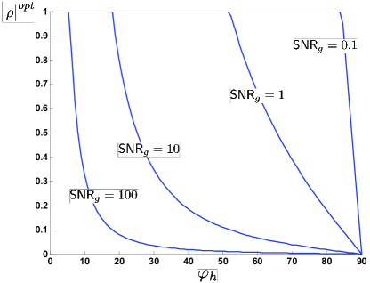
By defining the angle between channel vectors φh=arccos|𝐡1𝐡2|𝐡1𝐡2subscript𝜑superscriptsubscript𝐡1subscript𝐡2normsubscript𝐡1normsubscript𝐡2\varphi_{h}=\arccos\frac{{|{\mathbf{h}_{1}^{{\dagger}}\mathbf{h}_{2}}|}}{{||{\mathbf{h}_{1}}||||{\mathbf{h}_{2}}||}}, φh[0,π/2]subscript𝜑0𝜋2\varphi_{h}\in[0,\pi/2], and the geometric mean SNRgeo=Pr1Pr2𝐡1𝐡2subscriptSNR𝑔𝑒𝑜subscript𝑃𝑟1subscript𝑃𝑟2normsubscript𝐡1normsubscript𝐡2\textsf{SNR}_{geo}=\sqrt{P_{r1}P_{r2}}||{\mathbf{h}_{1}}||||{\mathbf{h}_{2}}||, the optimal correlation can be also expressed as

|ρ|opt=min(cosφhSNRgeosin2φh,1).superscript𝜌𝑜𝑝𝑡subscript𝜑subscriptSNR𝑔𝑒𝑜superscript2subscript𝜑1\left|\rho\right|^{opt}=\min\left({\frac{{\cos\varphi_{h}}}{{\textsf{SNR}_{geo}\sin^{2}\varphi_{h}}},1}\right).

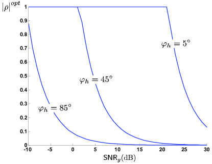
It is a monotonically decreasing function of φhsubscript𝜑\varphi_{h} and inversely proportional to SNRgeosubscriptSNR𝑔𝑒𝑜\textsf{SNR}_{geo}. In Fig. 3, |ρ|optsuperscript𝜌𝑜𝑝𝑡|\rho|^{opt} is drawn for different values of φhsubscript𝜑\varphi_{h} and SNRgeosubscriptSNR𝑔𝑒𝑜\textsf{SNR}_{geo}.

For a fixed SNRgeosubscriptSNR𝑔𝑒𝑜\textsf{SNR}_{geo} or for a fixed φhsubscript𝜑\varphi_{h}, there exists a threshold above which |ρ|opt<1superscript𝜌𝑜𝑝𝑡1|\rho|^{opt}<1 and below which |ρ|opt=1superscript𝜌𝑜𝑝𝑡1|\rho|^{opt}=1. The threshold is the solution of cosφh=SNRgeosin2φhsubscript𝜑subscriptSNR𝑔𝑒𝑜superscript2subscript𝜑\cos\varphi_{h}=\textsf{SNR}_{geo}\sin^{2}\varphi_{h}.

Remark 2

If 𝐡1subscript𝐡1\mathbf{h}_{1} and 𝐡2subscript𝐡2\mathbf{h}_{2} are orthogonal, then |ρ|opt=0superscript𝜌𝑜𝑝𝑡0|\rho|^{opt}=0. If channel vectors are orthogonal, the differential entropy of the received signal vector 𝐲dsubscript𝐲𝑑{\bf y}_{d} is maximized when xr1subscript𝑥𝑟1x_{r1} and xr2subscript𝑥𝑟2x_{r2} are uncorrelated. The resulting sum-rate is given by

maxρlogdet(𝐈+𝐇𝐐r𝐇)=log(1+Pr1𝐡12)+log(1+Pr2𝐡22).subscript𝜌𝐈subscript𝐇𝐐𝑟superscript𝐇1subscript𝑃𝑟1superscriptnormsubscript𝐡121subscript𝑃𝑟2superscriptnormsubscript𝐡22\mathop{\max}\limits_{\rho}\log\det(\mathbf{I+HQ}_{r}\mathbf{H}^{\mathbf{{\dagger}}})=\log(1+P_{r1}||{\mathbf{h}_{1}}||^{2})+\log(1+P_{r2}||{\mathbf{h}_{2}}||^{2}).

If 𝐡1subscript𝐡1\mathbf{h}_{1} and 𝐡2subscript𝐡2\mathbf{h}_{2} are parallel, then |ρ|opt=1superscript𝜌𝑜𝑝𝑡1|\rho|^{opt}=1. If channel vectors are parallel, the differential entropy of the received signal vector 𝐲dsubscript𝐲𝑑{\bf y}_{d} is maximized when xr1subscript𝑥𝑟1x_{r1} and xr2subscript𝑥𝑟2x_{r2} are fully correlated. The resulting sum-rate is given by

maxρlogdet(𝐈+𝐇𝐐r𝐇)=log(1+Pr1𝐡12+Pr2𝐡22+2Pr1Pr2|𝐡1𝐡2|).subscript𝜌𝐈subscript𝐇𝐐𝑟superscript𝐇1subscript𝑃𝑟1superscriptnormsubscript𝐡12subscript𝑃𝑟2superscriptnormsubscript𝐡222subscript𝑃𝑟1subscript𝑃𝑟2superscriptsubscript𝐡1subscript𝐡2\mathop{\max}\limits_{\rho}\log\det(\mathbf{I+HQ}_{r}\mathbf{H}^{\mathbf{{\dagger}}})=\log(1+P_{r1}||{\mathbf{h}_{1}}||^{2}+P_{r2}||{\mathbf{h}_{2}}||^{2}+2\sqrt{P_{r1}P_{r2}}|{\mathbf{h}_{1}^{\mathbf{{\dagger}}}\mathbf{h}_{2}}|).
Remark 3

For a fixed 𝐇𝐇\bf H, if either Pr1subscript𝑃𝑟1P_{r1} or Pr2subscript𝑃𝑟2P_{r2} are sufficiently small so that |ρ|opt=1superscript𝜌𝑜𝑝𝑡1|\rho|^{opt}=1, the signaling is optimal when the relay signals are perfectly correlated. If Pr1,Pr2>0subscript𝑃𝑟1subscript𝑃𝑟20P_{r1},P_{r2}>0 and either Pr1subscript𝑃𝑟1P_{r1} or Pr2subscript𝑃𝑟2P_{r2} are sufficiently large so that |ρ|opt=|𝐡1𝐡2|Pr1Pr2det(𝐇𝐇)<1superscript𝜌𝑜𝑝𝑡superscriptsubscript𝐡1subscript𝐡2subscript𝑃𝑟1subscript𝑃𝑟2superscript𝐇𝐇1|\rho|^{opt}=\frac{{|\mathbf{h}_{1}^{\dagger}\mathbf{h}_{2}|}}{{\sqrt{P_{r1}P_{r2}}\det\left(\mathbf{H^{\dagger}H}\right)}}<1, then |ρ|opt0superscript𝜌𝑜𝑝𝑡0|\rho|^{opt}\rightarrow 0 as either Pr1subscript𝑃𝑟1P_{r1} or Pr2subscript𝑃𝑟2P_{r2}\rightarrow\infty. If power is abundant, very small fraction of relay power needs to be allocated to common signals to satisfy optimality condition.

Remark 4

For N=1𝑁1N=1, the sum rate is maximized by |ρ|=1𝜌1|\rho|=1, i.e., α=β=|γ|=1𝛼𝛽𝛾1\alpha=\beta=|\gamma|=1 and ρ=(h1h2)𝜌superscriptsubscript1subscript2\angle\rho=\angle(h_{1}^{*}h_{2}) where 𝐇=[h1h2]𝐇delimited-[]subscript1subscript2missing-subexpressionmissing-subexpressionmissing-subexpressionmissing-subexpressionmissing-subexpressionmissing-subexpressionmissing-subexpressionmissing-subexpressionmissing-subexpressionmissing-subexpressionmissing-subexpressionmissing-subexpressionmissing-subexpressionmissing-subexpressionmissing-subexpressionmissing-subexpressionmissing-subexpressionmissing-subexpression\mathbf{H}=[{\begin{array}[]{*{20}c}{h_{1}}&{h_{2}}\\ \end{array}}].

By combining the optimal correlation condition with the achievable region expression in (15), we get the following result.

Theorem 3 (Maximum sum-rate subregion)

In the three-dimensional achievable region of a SIMO MAC given by (15), the maximum sum-rate subregion is a surface whose boundary is characterized by

sub(|ρ|opt)=|ρ|optα1(α)subscript𝑠𝑢𝑏superscript𝜌𝑜𝑝𝑡subscriptsuperscript𝜌𝑜𝑝𝑡𝛼1𝛼\displaystyle\mathcal{R}_{sub}\left({\left|\rho\right|^{opt}}\right)=\bigcup\limits_{\left|\rho\right|^{opt}\leq\sqrt{\alpha}\leq 1}{\mathcal{R}\left(\alpha\right)} (22)

where

(α)={(R1,R2,Rc)|R1log(1+α¯Pr1𝐡12)R2log(1+(1(|ρ|opt/α)2)Pr2𝐡22) for |ρ|opt>0R2log(1+Pr2𝐡22) for |ρ|opt=0R1+R2logdet(𝐈+𝐇𝐐rp𝐇)R1+R2+Rc=logdet(𝐈+𝐇𝐐r𝐇)}𝛼conditional-setsubscript𝑅1subscript𝑅2subscript𝑅𝑐subscript𝑅11¯𝛼subscript𝑃𝑟1superscriptdelimited-∥∥subscript𝐡12subscript𝑅211superscriptsuperscript𝜌𝑜𝑝𝑡𝛼2subscript𝑃𝑟2superscriptdelimited-∥∥subscript𝐡22 for superscript𝜌𝑜𝑝𝑡0subscript𝑅21subscript𝑃𝑟2superscriptdelimited-∥∥subscript𝐡22 for superscript𝜌𝑜𝑝𝑡0subscript𝑅1subscript𝑅2𝐈superscriptsubscript𝐇𝐐𝑟𝑝superscript𝐇subscript𝑅1subscript𝑅2subscript𝑅𝑐𝐈subscript𝐇𝐐𝑟superscript𝐇\displaystyle\mathcal{R}\left({\alpha}\right)=\left\{{\left({R_{1},R_{2},R_{c}}\right)\left|\begin{gathered}R_{1}\leq\log\left(1+\overline{\alpha}P_{r1}\left\|{\mathbf{h}_{1}}\right\|^{2}\right)\hfill\\ R_{2}\leq\log\left({1+(1-(|\rho|^{opt}/\sqrt{\alpha})^{2})P_{r2}\left\|{\mathbf{h}_{2}}\right\|^{2}}\right)\mbox{ for }|\rho|^{opt}>0\hfill\\ R_{2}\leq\log\left({1+P_{r2}\left\|{\mathbf{h}_{2}}\right\|^{2}}\right)\mbox{ for }|\rho|^{opt}=0\hfill\\ R_{1}+R_{2}\leq\log\det\left({\mathbf{I}+\mathbf{HQ}_{r}^{p}\mathbf{H}^{{\dagger}}}\right)\hfill\\ R_{1}+R_{2}+R_{c}=\log\det\left({\mathbf{I}+\mathbf{HQ}_{r}\mathbf{H}^{{\dagger}}}\right)\hfill\\ \end{gathered}\right.}\right\} (29)

where

𝐐rp=[(1α)Pr100(1(|ρ|opt/α)2)Pr2] for |ρ|opt>0,superscriptsubscript𝐐𝑟𝑝delimited-[]1𝛼subscript𝑃𝑟10missing-subexpressionmissing-subexpressionmissing-subexpressionmissing-subexpressionmissing-subexpressionmissing-subexpressionmissing-subexpressionmissing-subexpressionmissing-subexpressionmissing-subexpressionmissing-subexpressionmissing-subexpressionmissing-subexpressionmissing-subexpressionmissing-subexpressionmissing-subexpressionmissing-subexpressionmissing-subexpression01superscriptsuperscript𝜌𝑜𝑝𝑡𝛼2subscript𝑃𝑟2missing-subexpressionmissing-subexpressionmissing-subexpressionmissing-subexpressionmissing-subexpressionmissing-subexpressionmissing-subexpressionmissing-subexpressionmissing-subexpressionmissing-subexpressionmissing-subexpressionmissing-subexpressionmissing-subexpressionmissing-subexpressionmissing-subexpressionmissing-subexpressionmissing-subexpressionmissing-subexpression for superscript𝜌𝑜𝑝𝑡0\mathbf{Q}_{r}^{p}=\left[{\begin{array}[]{*{20}c}{(1-\alpha)P_{r1}}&0\\ 0&{(1-(|\rho|^{opt}/\sqrt{\alpha})^{2})P_{r2}}\\ \end{array}}\right]\mbox{ for }|\rho|^{opt}>0,
𝐐rp=[(1α)Pr100Pr2] for |ρ|opt=0,superscriptsubscript𝐐𝑟𝑝delimited-[]1𝛼subscript𝑃𝑟10missing-subexpressionmissing-subexpressionmissing-subexpressionmissing-subexpressionmissing-subexpressionmissing-subexpressionmissing-subexpressionmissing-subexpressionmissing-subexpressionmissing-subexpressionmissing-subexpressionmissing-subexpressionmissing-subexpressionmissing-subexpressionmissing-subexpressionmissing-subexpressionmissing-subexpressionmissing-subexpression0subscript𝑃𝑟2missing-subexpressionmissing-subexpressionmissing-subexpressionmissing-subexpressionmissing-subexpressionmissing-subexpressionmissing-subexpressionmissing-subexpressionmissing-subexpressionmissing-subexpressionmissing-subexpressionmissing-subexpressionmissing-subexpressionmissing-subexpressionmissing-subexpressionmissing-subexpressionmissing-subexpressionmissing-subexpression for superscript𝜌𝑜𝑝𝑡0\mathbf{Q}_{r}^{p}=\left[{\begin{array}[]{*{20}c}{(1-\alpha)P_{r1}}&0\\ 0&{P_{r2}}\\ \end{array}}\right]\mbox{ for }|\rho|^{opt}=0,
𝐐r=[Pr1|ρ|optej𝐡1𝐡2Pr1Pr2|ρ|optej𝐡1𝐡2Pr1Pr2Pr2].subscript𝐐𝑟delimited-[]subscript𝑃𝑟1superscript𝜌𝑜𝑝𝑡superscript𝑒𝑗superscriptsubscript𝐡1subscript𝐡2subscript𝑃𝑟1subscript𝑃𝑟2missing-subexpressionmissing-subexpressionmissing-subexpressionmissing-subexpressionmissing-subexpressionmissing-subexpressionmissing-subexpressionmissing-subexpressionmissing-subexpressionmissing-subexpressionmissing-subexpressionmissing-subexpressionmissing-subexpressionmissing-subexpressionmissing-subexpressionmissing-subexpressionmissing-subexpressionmissing-subexpressionsuperscript𝜌𝑜𝑝𝑡superscript𝑒𝑗superscriptsubscript𝐡1subscript𝐡2subscript𝑃𝑟1subscript𝑃𝑟2subscript𝑃𝑟2missing-subexpressionmissing-subexpressionmissing-subexpressionmissing-subexpressionmissing-subexpressionmissing-subexpressionmissing-subexpressionmissing-subexpressionmissing-subexpressionmissing-subexpressionmissing-subexpressionmissing-subexpressionmissing-subexpressionmissing-subexpressionmissing-subexpressionmissing-subexpressionmissing-subexpressionmissing-subexpression\mathbf{Q}_{r}=\left[{\begin{array}[]{*{20}c}{P_{r1}}&{|\rho|^{opt}e^{j\angle{\mathbf{h}_{1}^{\dagger}\mathbf{h}_{2}}}\sqrt{P_{r1}P_{r2}}}\\ {|\rho|^{opt}e^{-j\angle{\mathbf{h}_{1}^{\dagger}\mathbf{h}_{2}}}\sqrt{P_{r1}P_{r2}}}&{P_{r2}}\\ \end{array}}\right].


Proof:

To satisfy the optimal correlation, 0|ρ|opt=|γ|αβ10superscript𝜌𝑜𝑝𝑡𝛾𝛼𝛽10\leq|\rho|^{opt}=|\gamma|\sqrt{\alpha\beta}\leq 1, |γ|𝛾|\gamma|, α𝛼\sqrt{\alpha} and β𝛽\sqrt{\beta} should be in the range [|ρ|opt,1]superscript𝜌𝑜𝑝𝑡1[|\rho|^{opt},1]. In (15), by setting |γ|=1𝛾1|\gamma|=1, and β=(|ρ|opt/α)2𝛽superscriptsuperscript𝜌𝑜𝑝𝑡𝛼2\beta=(|\rho|^{opt}/\sqrt{\alpha})^{2} for |ρ|opt>0superscript𝜌𝑜𝑝𝑡0|\rho|^{opt}>0 or β=0𝛽0\beta=0 for |ρ|opt=0superscript𝜌𝑜𝑝𝑡0|\rho|^{opt}=0, and by taking union over |ρ|optα1superscript𝜌𝑜𝑝𝑡𝛼1|\rho|^{opt}\leq\sqrt{\alpha}\leq 1, we characterize the boundary of the maximum sum-rate surface. ∎

Example 1 (Close-to-parallel channel vectors)

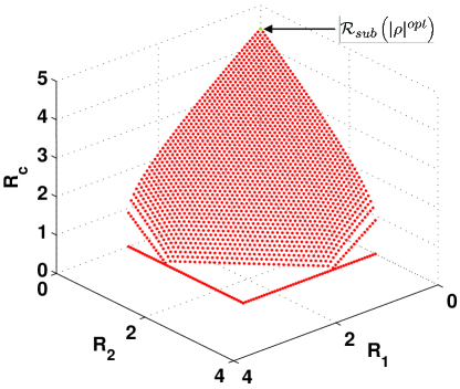
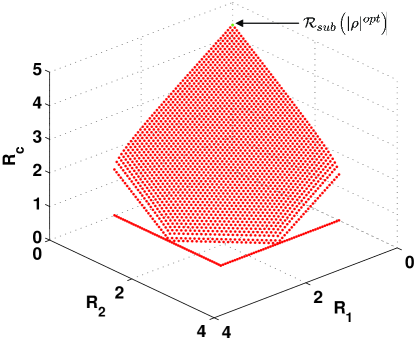
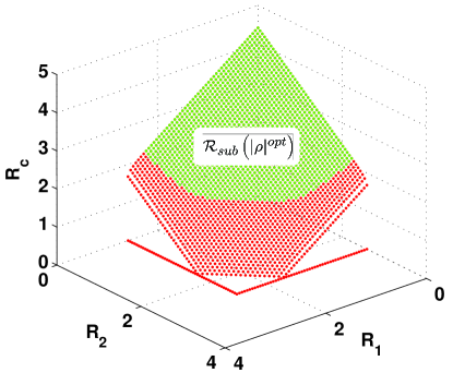
If |ρ|opt=1superscript𝜌𝑜𝑝𝑡1|\rho|^{opt}=1, it is required for relays to set α=β=|γ|=1𝛼𝛽𝛾1\alpha=\beta=|\gamma|=1. Substituting this condition into (15), we get the expression for the maximum sum-rate subregion which is a single point given by

{(R1,R2,Rc)|R1=0,R2=0,Rc=log(1+Pr1𝐡12+Pr2𝐡22+2Pr1Pr2|𝐡1𝐡2|)}.conditional-setsubscript𝑅1subscript𝑅2subscript𝑅𝑐formulae-sequencesubscript𝑅10formulae-sequencesubscript𝑅20subscript𝑅𝑐1subscript𝑃𝑟1superscriptdelimited-∥∥subscript𝐡12subscript𝑃𝑟2superscriptdelimited-∥∥subscript𝐡222subscript𝑃𝑟1subscript𝑃𝑟2superscriptsubscript𝐡1subscript𝐡2\left\{{\left({R_{1},R_{2},R_{c}}\right)\left|\begin{gathered}R_{1}=0,R_{2}=0,\hfill\\ R_{c}=\log(1+P_{r1}\left\|{\mathbf{h}_{1}}\right\|^{2}+P_{r2}\left\|{\mathbf{h}_{2}}\right\|^{2}+2\sqrt{P_{r1}P_{r2}}|{\mathbf{h}_{1}^{{\dagger}}\mathbf{h}_{2}}|)\hfill\\ \end{gathered}\right.}\right\}.

The example achievable rate region is drawn in Fig. 4 (a) and (b), and the maximum sum-rate point (0,0,Rsum,MACmax)00superscriptsubscript𝑅𝑠𝑢𝑚𝑀𝐴𝐶𝑚𝑎𝑥(0,0,R_{sum,MAC}^{max}) is on the Rcsubscript𝑅𝑐R_{c} axis.

Example 2 (Orthogonal channel vectors)

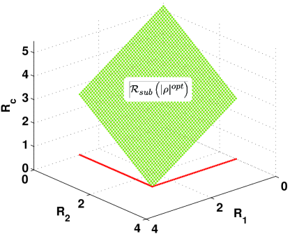
If |ρ|opt=0superscript𝜌𝑜𝑝𝑡0\left|\rho\right|^{opt}=0, at least one of α𝛼\alpha, β𝛽\beta and |γ|𝛾|\gamma| must be zero. We get the expression for the maximum sum-rate subregion given by

{(R1,R2,Rc)|R1log(1+Pr1𝐡12)R2log(1+Pr2𝐡22)R1+R2+Rci=1,2log(1+Pri𝐡i2)}.conditional-setsubscript𝑅1subscript𝑅2subscript𝑅𝑐subscript𝑅11subscript𝑃𝑟1superscriptdelimited-∥∥subscript𝐡12subscript𝑅21subscript𝑃𝑟2superscriptdelimited-∥∥subscript𝐡22subscript𝑅1subscript𝑅2subscript𝑅𝑐subscript𝑖121subscript𝑃𝑟𝑖superscriptdelimited-∥∥subscript𝐡𝑖2\left\{{\left({R_{1},R_{2},R_{c}}\right)\left|\begin{gathered}R_{1}\leq\log(1+P_{r1}\left\|{\mathbf{h}_{1}}\right\|^{2})\hfill\\ R_{2}\leq\log(1+P_{r2}\left\|{\mathbf{h}_{2}}\right\|^{2})\hfill\\ R_{1}+R_{2}+R_{c}\leq\sum\limits_{i=1,2}{\log(1+P_{ri}\left\|{\mathbf{h}_{i}}\right\|^{2})}\hfill\\ \end{gathered}\right.}\right\}.

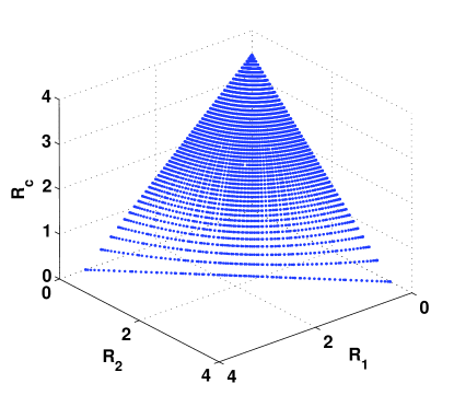
As it is shown in Fig. 4 (d), the maximum sum-rate surface is the square connecting four points: (R1max,R2max,0)superscriptsubscript𝑅1𝑚𝑎𝑥superscriptsubscript𝑅2𝑚𝑎𝑥0(R_{1}^{max},R_{2}^{max},0), (R1max,0,Rsum,MACmaxR1max)superscriptsubscript𝑅1𝑚𝑎𝑥0superscriptsubscript𝑅𝑠𝑢𝑚𝑀𝐴𝐶𝑚𝑎𝑥superscriptsubscript𝑅1𝑚𝑎𝑥(R_{1}^{max},0,R_{sum,MAC}^{max}-R_{1}^{max}), (0,R2max,Rsum,MACmaxR2max)0superscriptsubscript𝑅2𝑚𝑎𝑥superscriptsubscript𝑅𝑠𝑢𝑚𝑀𝐴𝐶𝑚𝑎𝑥superscriptsubscript𝑅2𝑚𝑎𝑥(0,R_{2}^{max},R_{sum,MAC}^{max}-R_{2}^{max}), and (0,0,Rsum,MACmax)00superscriptsubscript𝑅𝑠𝑢𝑚𝑀𝐴𝐶𝑚𝑎𝑥(0,0,R_{sum,MAC}^{max}), where Rimaxsuperscriptsubscript𝑅𝑖𝑚𝑎𝑥R_{i}^{max} denotes the maximum rate that can be achieved by each message set. In the subregion, for any fixed R1subscript𝑅1R_{1} and R2subscript𝑅2R_{2}, we can find Rcsubscript𝑅𝑐R_{c} such that Rsum,MACmax=R1+R2+Rcsuperscriptsubscript𝑅𝑠𝑢𝑚𝑀𝐴𝐶𝑚𝑎𝑥subscript𝑅1subscript𝑅2subscript𝑅𝑐R_{sum,MAC}^{max}=R_{1}+R_{2}+R_{c}.

IV-B Impact of Common Information Signaling

Let us discuss how much benefit we can get by having the common information for N2𝑁2N\geq 2 case. If the source transmits only the private signal to relays, i.e. Rc=0subscript𝑅𝑐0R_{c}=0, the best strategy relays can do is to have diagonal covariance matrix with individual peak power 𝐐rdiag=diag[Pr1,Pr2]superscriptsubscript𝐐𝑟𝑑𝑖𝑎𝑔𝑑𝑖𝑎𝑔subscript𝑃𝑟1subscript𝑃𝑟2\mathbf{Q}_{r}^{diag}=diag[P_{r1},P_{r2}]. Let 𝐐roptsuperscriptsubscript𝐐𝑟𝑜𝑝𝑡\mathbf{Q}_{r}^{opt} denote optimal covariance matrix with sum rate maximizing magnitude and phase angle of ρ𝜌\rho derived above. Then, we get the following result.

Lemma 2 (Benefit of correlation)

logdet(𝐈+𝐇𝐐rdiag𝐇)logdet(𝐈+𝐇𝐐ropt𝐇)𝐈superscriptsubscript𝐇𝐐𝑟𝑑𝑖𝑎𝑔superscript𝐇𝐈superscriptsubscript𝐇𝐐𝑟𝑜𝑝𝑡superscript𝐇\log\det\left({{\bf I}+{\bf HQ}_{r}^{diag}{\bf H}^{\dagger}}\right)\leq\log\det\left({{\bf I}+{\bf HQ}_{r}^{opt}{\bf H}^{\dagger}}\right) with equality if and only if 𝐡1𝐡2=0superscriptsubscript𝐡1subscript𝐡20\mathbf{h}_{1}^{\dagger}\mathbf{h}_{2}=0. The increase in SNR by having 𝐐roptsuperscriptsubscript𝐐𝑟𝑜𝑝𝑡\mathbf{Q}_{r}^{opt} is given by

ΔSNR={|𝐡1𝐡2|2det(𝐇𝐇),|ρ|opt<12Pr1Pr2|𝐡1𝐡2|,|ρ|opt=1.ΔSNRcasessuperscriptsuperscriptsubscript𝐡1subscript𝐡22superscript𝐇𝐇superscript𝜌𝑜𝑝𝑡1missing-subexpressionmissing-subexpressionmissing-subexpressionmissing-subexpressionmissing-subexpressionmissing-subexpressionmissing-subexpressionmissing-subexpressionmissing-subexpressionmissing-subexpressionmissing-subexpressionmissing-subexpressionmissing-subexpressionmissing-subexpressionmissing-subexpressionmissing-subexpressionmissing-subexpressionmissing-subexpression2subscript𝑃𝑟1subscript𝑃𝑟2superscriptsubscript𝐡1subscript𝐡2superscript𝜌𝑜𝑝𝑡1missing-subexpressionmissing-subexpressionmissing-subexpressionmissing-subexpressionmissing-subexpressionmissing-subexpressionmissing-subexpressionmissing-subexpressionmissing-subexpressionmissing-subexpressionmissing-subexpressionmissing-subexpressionmissing-subexpressionmissing-subexpressionmissing-subexpressionmissing-subexpressionmissing-subexpressionmissing-subexpression\Delta\textsf{SNR}=\left\{{\begin{array}[]{*{20}c}{\frac{{|\mathbf{h}_{1}^{{\dagger}}\mathbf{h}_{2}|^{2}}}{{\det(\mathbf{H^{{\dagger}}H})}},}&{|\rho|^{opt}<1}\\ {2\sqrt{P_{r1}P_{r2}}|{\mathbf{h}_{1}^{\dagger}\mathbf{h}_{2}}|,}&{|\rho|^{opt}=1}\\ \end{array}}\right..
Proof:

: It is sufficient to show that the sum-rate is a quadratic and concave function of |ρ|𝜌|\rho|, and is monotonically increasing for 0|ρ||ρ|opt0𝜌superscript𝜌𝑜𝑝𝑡0\leq|\rho|\leq|\rho|^{opt}. The function has its minimum at |ρ|=0𝜌0|\rho|=0 since |ρ|𝜌|\rho| is non-negative. When the channel vectors are orthogonal, the suboptimality vanishes since |ρ|opt=0superscript𝜌𝑜𝑝𝑡0|\rho|^{opt}=0. The SNR increase can be directly calculated using the result in Lemma 1. ∎

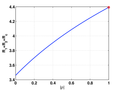
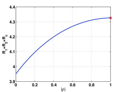
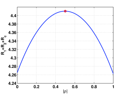
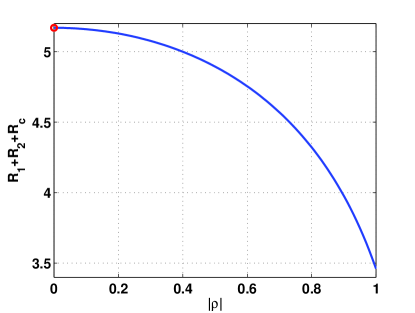
When the channel column vectors 𝐡1subscript𝐡1\mathbf{h}_{1} and 𝐡2subscript𝐡2\mathbf{h}_{2} are close to orthogonal, 𝐐rdiagsuperscriptsubscript𝐐𝑟𝑑𝑖𝑎𝑔\mathbf{Q}_{r}^{diag} is almost as good as 𝐐roptsuperscriptsubscript𝐐𝑟𝑜𝑝𝑡\mathbf{Q}_{r}^{opt}. However, when 𝐡1subscript𝐡1\mathbf{h}_{1} and 𝐡2subscript𝐡2\mathbf{h}_{2} are close to parallel, the sum rate by having 𝐐roptsuperscriptsubscript𝐐𝑟𝑜𝑝𝑡\mathbf{Q}_{r}^{opt} at relays shows considerable increase from that by having 𝐐rdiagsuperscriptsubscript𝐐𝑟𝑑𝑖𝑎𝑔\mathbf{Q}_{r}^{diag}. The gain coming from optimal correlation becomes very large at low SNR. Fig. 5 shows the examples.

With common information coming from the source, we can introduce correlation between relays, and they act as if they are in cooperation. The resulting SIMO MAC behaves like a point-to-point MIMO channel with per-antenna power constraint.

Here, we can see that there is a minimum required Rcsubscript𝑅𝑐R_{c} that needs to be transmitted from the source to relays for achieving maximum sum-rate in the second hop.

Theorem 4 (Threshold of Rcsubscript𝑅𝑐R_{c})

In the SIMO MAC with common information, the threshold of Rcsubscript𝑅𝑐R_{c} above which a maximum sum-rate point can exist is characterized by

Rcth=logdet(𝐈+𝐇𝐐ropt𝐇)det(𝐈+𝐇𝐐rk𝐇)superscriptsubscript𝑅𝑐𝑡𝐈superscriptsubscript𝐇𝐐𝑟𝑜𝑝𝑡superscript𝐇𝐈superscriptsubscript𝐇𝐐𝑟𝑘superscript𝐇R_{c}^{th}=\log\frac{{\det\left({\mathbf{I}+\mathbf{HQ}_{r}^{opt}\mathbf{H}^{{\dagger}}}\right)}}{{\det\left({\mathbf{I}+\mathbf{HQ}_{r}^{k}\mathbf{H}^{{\dagger}}}\right)}}\hfill\\

where 𝐐rk=diag[(1k|ρ|opt)Pr1,(1k1|ρ|opt)Pr2]superscriptsubscript𝐐𝑟𝑘𝑑𝑖𝑎𝑔1𝑘superscript𝜌𝑜𝑝𝑡subscript𝑃𝑟11superscript𝑘1superscript𝜌𝑜𝑝𝑡subscript𝑃𝑟2\mathbf{Q}_{r}^{k}=diag[(1-k|\rho|^{opt})P_{r1},(1-k^{-1}|\rho|^{opt})P_{r2}] and k=Pr2𝐡22+Pr1Pr2det(𝐇𝐇)Pr1𝐡12+Pr1Pr2det(𝐇𝐇)𝑘subscript𝑃𝑟2superscriptnormsubscript𝐡22subscript𝑃𝑟1subscript𝑃𝑟2superscript𝐇𝐇subscript𝑃𝑟1superscriptnormsubscript𝐡12subscript𝑃𝑟1subscript𝑃𝑟2superscript𝐇𝐇k=\sqrt{\frac{{P_{r2}\left\|{\mathbf{h}_{2}}\right\|^{2}+P_{r1}P_{r2}\det(\mathbf{H}^{{\dagger}}\mathbf{H})}}{{P_{r1}\left\|{\mathbf{h}_{1}}\right\|^{2}+P_{r1}P_{r2}\det(\mathbf{H}^{{\dagger}}\mathbf{H})}}}.

Proof:

In the maximum sum-rate subregion in (29), after evaluating det()\det(\cdot) operation, we get the expression for R1+R2subscript𝑅1subscript𝑅2R_{1}+R_{2} given by

R1+R2log(1+α¯Pr1𝐡12+(1|ρ|2α)Pr2𝐡22+(1α+|ρ|2|ρ|2α)Pr1Pr2det(𝐇𝐇)).subscript𝑅1subscript𝑅21¯𝛼subscript𝑃𝑟1superscriptdelimited-∥∥subscript𝐡121superscript𝜌2𝛼subscript𝑃𝑟2superscriptdelimited-∥∥subscript𝐡221𝛼superscript𝜌2superscript𝜌2𝛼subscript𝑃𝑟1subscript𝑃𝑟2superscript𝐇𝐇\displaystyle\begin{gathered}R_{1}+R_{2}\leq\hfill\\ \log\left({1+\overline{\alpha}P_{r1}\left\|{\mathbf{h}_{1}}\right\|^{2}+\left({1-\frac{{\left|\rho\right|^{2}}}{\alpha}}\right)P_{r2}\left\|{\mathbf{h}_{2}}\right\|^{2}+\left({1-\alpha+\left|\rho\right|^{2}-\frac{{\left|\rho\right|^{2}}}{\alpha}}\right)P_{r1}P_{r2}\det(\mathbf{H}^{\mathbf{{\dagger}}}\mathbf{H})}\right).\end{gathered}

It is straightforward to check that the maximum of R1+R2subscript𝑅1subscript𝑅2R_{1}+R_{2} is given by

maxα(R1+R2)=logdet(𝐈+𝐇𝐐rk𝐇)subscript𝛼subscript𝑅1subscript𝑅2𝐈superscriptsubscript𝐇𝐐𝑟𝑘superscript𝐇\displaystyle\begin{gathered}\mathop{\max}\limits_{\alpha}(R_{1}+R_{2})=\log\det(\mathbf{I+HQ}_{r}^{k}\mathbf{H}^{{\dagger}})\end{gathered}

with 𝐐rksuperscriptsubscript𝐐𝑟𝑘\mathbf{Q}_{r}^{k} given in the theorem statement. Finally, Rcth=Rsum,MACmaxmaxα(R1+R2)superscriptsubscript𝑅𝑐𝑡superscriptsubscript𝑅𝑠𝑢𝑚𝑀𝐴𝐶𝑚𝑎𝑥subscript𝛼subscript𝑅1subscript𝑅2R_{c}^{th}=R_{sum,MAC}^{max}-\mathop{\max}\limits_{\alpha}(R_{1}+R_{2}) results in the minimum possible value of Rcsubscript𝑅𝑐R_{c} while staying in the maximum sum-rate subregion. ∎

IV-C SISO MAC versus SIMO MAC

Optimal signaling at DF relays depends on the channel condition. For a SISO MAC with a single antenna at the destination (N=1𝑁1N=1), the sum-rate is maximized by α=β=|γ|=1𝛼𝛽𝛾1\alpha=\beta=|\gamma|=1 so that R1=R2=0subscript𝑅1subscript𝑅20R_{1}=R_{2}=0 regardless of the channel and power constraints. This is the case when all the power is allocated to the common signal at both relays and they add up coherently at the destination. It is desired for the source to transmit as much common information to relays as possible, and this strategy maximizes the source-to-destination sum-rate. Even when N2𝑁2N\geq 2, if 𝐡1subscript𝐡1{\bf h}_{1} and 𝐡2subscript𝐡2{\bf h}_{2} are close to parallel in the sense that det(𝐇𝐇)superscript𝐇𝐇\det(\bf{H^{\dagger}H}) is small and |ρ|opt=1superscript𝜌𝑜𝑝𝑡1|\rho|^{opt}=1, fully correlated relay signals are still optimal.

In contrast, with multiple antennas at the destination (N2𝑁2N\geq 2) and |ρ|opt<1superscript𝜌𝑜𝑝𝑡1|\rho|^{opt}<1, sum-rate maximizing α𝛼\alpha and β𝛽\beta depend on both the channel matrix 𝐇𝐇\mathbf{H} and relay power constraints. Any combination of power allocation factors at relays such that |γ|αβ=|𝐡1𝐡2|Pr1Pr2det(𝐇𝐇)<1𝛾𝛼𝛽superscriptsubscript𝐡1subscript𝐡2subscript𝑃𝑟1subscript𝑃𝑟2superscript𝐇𝐇1|\gamma|\sqrt{\alpha\beta}=\frac{{|\mathbf{h}_{1}^{\dagger}\mathbf{h}_{2}|}}{{\sqrt{P_{r1}P_{r2}}\det(\bf{H^{\dagger}H})}}<1 together with optimal rotation angle γ=𝐡1𝐡2𝛾superscriptsubscript𝐡1subscript𝐡2\angle\gamma=\angle\mathbf{h}_{1}^{\dagger}\mathbf{h}_{2} can maximize the sum rate of a SIMO MAC. In this case, the source needs to transmit just the right amount of common information so that signals at two relays are optimally correlated and the source-to-destination sum-rate is maximized.

IV-D The First Hop: MISO BC with Common Information

In [1], the first hop is a degraded scalar BC where one relay with higher SNR can decode both its intend signal and the signal for the other relay by doing superposition coding and successive interference cancellation. In this case, correlation between relay input signals are naturally introduced. In contrast, our first hop is a non-degraded vector broadcast channel that makes it possible to send private signals, each decodable by one of the relays, as well as a common signal decodable by both relays. For this class of channels, the three dimensional capacity region is not known, but a good achievable region combining dirty paper coding (DPC)[13] and superposition was studied in [10, 11, 12] which we also use here.

In this scheme, the transmitting signal 𝐱ssubscript𝐱𝑠{\bf x}_{s} is a superposition of three independent signals 𝐱1subscript𝐱1{\bf x}_{1}, 𝐱2subscript𝐱2{\bf x}_{2} and 𝐱csubscript𝐱𝑐{\bf x}_{c}, i.e., 𝐱s=𝐱1+𝐱2+𝐱csubscript𝐱𝑠subscript𝐱1subscript𝐱2subscript𝐱𝑐{\bf x}_{s}={\bf x}_{1}+{\bf x}_{2}+{\bf x}_{c}, where 𝐱1,𝐱2,𝐱cN×1subscript𝐱1subscript𝐱2subscript𝐱𝑐superscriptN1{\bf x}_{1},{\bf x}_{2},{\bf x}_{c}\in{\mathbb{C}}^{{\rm N}\times{\rm 1}} denote the signals intended for relay 1, for relay 2 and for both relays, i.e., the common message, respectively. We assume Gaussian signaling for all signals. Input covariance matrix is 𝐐s=𝐐1+𝐐2+𝐐csubscript𝐐𝑠subscript𝐐1subscript𝐐2subscript𝐐𝑐\mathbf{Q}_{s}=\mathbf{Q}_{1}+\mathbf{Q}_{2}+\mathbf{Q}_{c}, where 𝐐j=𝔼[𝐱j𝐱j]subscript𝐐𝑗𝔼delimited-[]subscript𝐱𝑗superscriptsubscript𝐱𝑗\mathbf{Q}_{j}=\mathbb{E}[{\mathbf{x}_{j}\mathbf{x}_{j}^{\dagger}}], j{1,2,c}𝑗12𝑐j\in\{1,2,c\}.

Common information is decoded at both relays before decoding private messages. Private messages are encoded using dirty paper coding, i.e., the private message for relay 1 is first encoded as 𝐱1subscript𝐱1\mathbf{x}_{1}, and the private message for relay 2 is then encoded as 𝐱2subscript𝐱2\mathbf{x}_{2} using 𝐱1subscript𝐱1\mathbf{x}_{1} as side information so that 𝐱2subscript𝐱2\mathbf{x}_{2} can be decoded at relay 2 without interference from 𝐱1subscript𝐱1\mathbf{x}_{1}. The encoding order can be reversed. With this scheme, an achievable rate region is given by

BC(Ps)=Co(π,𝐐s:tr(𝐐s)Ps(π,𝐐s))subscript𝐵𝐶subscript𝑃𝑠𝐶𝑜subscript:𝜋subscript𝐐𝑠trsubscript𝐐𝑠subscript𝑃𝑠𝜋subscript𝐐𝑠\displaystyle\mathcal{R}_{BC}\left(P_{s}\right)=Co\left({\bigcup\limits_{\pi,\mathbf{Q}_{s}:\text{tr}\left({\mathbf{Q}_{s}}\right)\leq P_{s}}{\mathcal{R}\left({\pi,\mathbf{Q}_{s}}\right)}}\right) (33)

where (π,𝐐s)𝜋subscript𝐐𝑠{\mathcal{R}\left({\pi,\mathbf{Q}_{s}}\right)} is the achievable region for a given encoding order π{π12,π21}𝜋subscript𝜋12subscript𝜋21\pi\in\left\{{\pi_{12},\pi_{21}}\right\} and input covariance matrix 𝐐ssubscript𝐐𝑠\mathbf{Q}_{s}, where Co()𝐶𝑜Co(\cdot) is the convex hull operator. If 𝐱2subscript𝐱2\mathbf{x}_{2} is encoded first, for example, then we have

(π12,𝐐s)={(R1,R2,Rc)|R1log(1+𝐠1𝐐1𝐠1),R2log(1+𝐠2𝐐2𝐠21+𝐠2𝐐1𝐠2),Rcmini{1,2}log(1+𝐠i𝐐c𝐠i1+𝐠i(𝐐1+𝐐2)𝐠i)}.\displaystyle\mathcal{R}\left({\pi_{12},\mathbf{Q}_{s}}\right)=\left\{{\left({R_{1},R_{2},R_{c}}\right)\left|{\begin{array}[]{*{20}c}{R_{1}\leq\log\left(1+{\mathbf{g}_{1}\mathbf{Q}_{1}\mathbf{g}_{1}^{\dagger}}\right),\hfill}\\ {R_{2}\leq\log\left(1+{\frac{{\mathbf{g}_{2}\mathbf{Q}_{2}\mathbf{g}_{2}^{\dagger}}}{{1+\mathbf{g}_{2}\mathbf{Q}_{1}\mathbf{g}_{2}^{\dagger}}}}\right),\hfill}\\ {R_{c}\leq\mathop{\min}\limits_{i\in\left\{{1,2}\right\}}\log\left(1+{\frac{{\mathbf{g}_{i}\mathbf{Q}_{c}\mathbf{g}_{i}^{\dagger}}}{{1+\mathbf{g}_{i}\left({\mathbf{Q}_{1}+\mathbf{Q}_{2}}\right)\mathbf{g}_{i}^{\dagger}}}}\right)\hfill}\\ \end{array}}\right.}\right\}. (37)

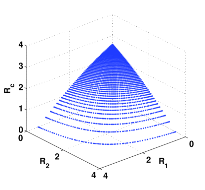
Fig. 6. (a) depicts an example of an achievable region where two row vectors of 𝐆𝐆\bf G are parallel and linearly dependent so that 𝐆𝐆\bf G is ill-conditioned and rank-deficient. Note that in the figures, φg=arccos|𝐠1𝐠2|𝐠1𝐠2subscript𝜑𝑔subscript𝐠1superscriptsubscript𝐠2normsubscript𝐠1normsubscript𝐠2\varphi_{g}=\arccos\frac{{|{\mathbf{g}_{1}\mathbf{g}_{2}^{{\dagger}}}|}}{{\left\|{\mathbf{g}_{1}}\right\|\left\|{\mathbf{g}_{2}}\right\|}}. One can see that the maximum sum-rate surface is a plane connecting three points: (R1,BCmax,0,0)superscriptsubscript𝑅1𝐵𝐶𝑚𝑎𝑥00(R_{1,BC}^{max},0,0), (0,R2,BCmax,0)0superscriptsubscript𝑅2𝐵𝐶𝑚𝑎𝑥0(0,R_{2,BC}^{max},0), and (0,0,Rc,BCmax)00superscriptsubscript𝑅𝑐𝐵𝐶𝑚𝑎𝑥(0,0,R_{c,BC}^{max}) where Rj,BCmaxsuperscriptsubscript𝑅𝑗𝐵𝐶𝑚𝑎𝑥R_{j,BC}^{max} denotes the maximum rate achieved by allocating all power to 𝐱jsubscript𝐱𝑗\mathbf{x}_{j} so that 𝐐j=𝐐ssubscript𝐐𝑗subscript𝐐𝑠\mathbf{Q}_{j}=\mathbf{Q}_{s}:

Ri,BCmax=max𝐐slog(1+𝐠i𝐐s𝐠i)=log(1+Ps𝐠i2)superscriptsubscript𝑅𝑖𝐵𝐶𝑚𝑎𝑥subscriptsubscript𝐐𝑠1subscript𝐠𝑖subscript𝐐𝑠superscriptsubscript𝐠𝑖1subscript𝑃𝑠superscriptnormsubscript𝐠𝑖2R_{i,BC}^{max}=\mathop{\max}\limits_{\mathbf{Q}_{s}}\log\left(1+{\mathbf{g}_{i}\mathbf{Q}_{s}\mathbf{g}_{i}^{\dagger}}\right)=\log\left({1+P_{s}\left\|{\mathbf{g}_{i}}\right\|^{2}}\right)
Rc,BCmax=max𝐐sminilog(1+𝐠i𝐐s𝐠i)=minilog(1+Ps𝐠i2)superscriptsubscript𝑅𝑐𝐵𝐶𝑚𝑎𝑥subscriptsubscript𝐐𝑠subscript𝑖1subscript𝐠𝑖subscript𝐐𝑠superscriptsubscript𝐠𝑖subscript𝑖1subscript𝑃𝑠superscriptnormsubscript𝐠𝑖2R_{c,BC}^{max}={\mathop{\max}\limits_{\mathbf{Q}_{s}}\mathop{\min}\limits_{i}\log(1+{\mathbf{g}_{i}\mathbf{Q}_{s}\mathbf{g}_{i}^{\dagger}})}=\mathop{\min}\limits_{i}\log\left({1+P_{s}\left\|{\mathbf{g}_{i}}\right\|^{2}}\right)

where i{1,2}𝑖12i\in\{1,2\}. In this specific example, the channel is symmetric in the sense that 𝐠1=𝐠2normsubscript𝐠1normsubscript𝐠2\left\|\mathbf{g}_{1}\right\|=\left\|\mathbf{g}_{2}\right\|. In fact, this is the only case where having common information does not incur sum-rate penalty.

As the opposite extreme, Fig. 6. (b) depicts an example of an achievable region where two row vectors of 𝐆𝐆\bf G are orthogonal and linearly independent so that 𝐆𝐆\bf G is well-conditioned and full-rank. In the symmetric example, the point that achieves the maximum sum-rate

Rsum,BCmax=log(1+Ps2𝐠1)+log(1+Ps2𝐠2)superscriptsubscript𝑅𝑠𝑢𝑚𝐵𝐶𝑚𝑎𝑥1subscript𝑃𝑠2normsubscript𝐠11subscript𝑃𝑠2normsubscript𝐠2R_{sum,BC}^{max}=\log(1+\frac{{P_{s}}}{{2}}\|\mathbf{g}_{1}\|)+\log(1+\frac{{P_{s}}}{{2}}\|\mathbf{g}_{2}\|)

is on the line R1=R2subscript𝑅1subscript𝑅2R_{1}=R_{2} and Rc=0subscript𝑅𝑐0R_{c}=0. The point that has the minimum sum-rate on the boundary is on the Rcsubscript𝑅𝑐R_{c} axis, i.e., R1=R2=0subscript𝑅1subscript𝑅20R_{1}=R_{2}=0 and

Rc,BCmax=max𝐐sminilog(1+𝐠i𝐐s𝐠i)=log(1+Ps2𝐠1)=log(1+Ps2𝐠2)superscriptsubscript𝑅𝑐𝐵𝐶𝑚𝑎𝑥subscriptsubscript𝐐𝑠subscript𝑖1subscript𝐠𝑖subscript𝐐𝑠superscriptsubscript𝐠𝑖1subscript𝑃𝑠2normsubscript𝐠11subscript𝑃𝑠2normsubscript𝐠2R_{c,BC}^{max}={\mathop{\max}\limits_{\mathbf{Q}_{s}}\mathop{\min}\limits_{i}\log(1+{\mathbf{g}_{i}\mathbf{Q}_{s}\mathbf{g}_{i}^{\dagger}})}=\log(1+\frac{{P_{s}}}{{2}}\|\mathbf{g}_{1}\|)=\log(1+\frac{{P_{s}}}{{2}}\|\mathbf{g}_{2}\|)

where we can see the sum-rate penalty due to beamforming inefficiency.

Note that the maximum sum-rate points of a MISO BC are always on the R1R2subscript𝑅1subscript𝑅2R_{1}-R_{2} plane. In fact, they correspond to the dominant face of the two user BC achievable region by DPC without common information.

IV-E Achievable Rate by DF

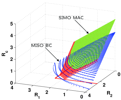
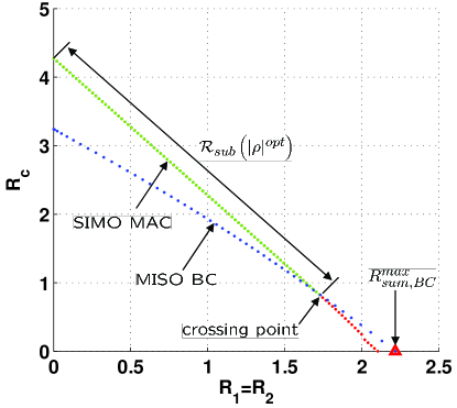
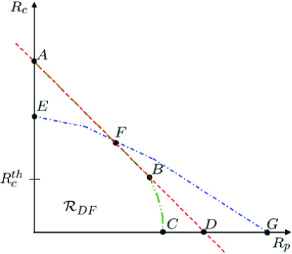
For the GPRN drawn in Fig. 1, a triplet (R1,R2,Rc)subscript𝑅1subscript𝑅2subscript𝑅𝑐\left(R_{1},R_{2},R_{c}\right) is said to be achievable by DF if it belongs to the intersection of the rate regions of the first hop MISO BC and the second hop SIMO MAC. In this context, the maximum rate by DF can be defined by

RDFmax=max(R1,R2,Rc)DFR1+R2+Rcsuperscriptsubscript𝑅𝐷𝐹𝑚𝑎𝑥subscriptsubscript𝑅1subscript𝑅2subscript𝑅𝑐subscript𝐷𝐹subscript𝑅1subscript𝑅2subscript𝑅𝑐\displaystyle R_{DF}^{max}=\mathop{\max}\limits_{\left({R_{1},R_{2},R_{c}}\right)\in\mathcal{R}_{DF}}R_{1}+R_{2}+R_{c} (38)

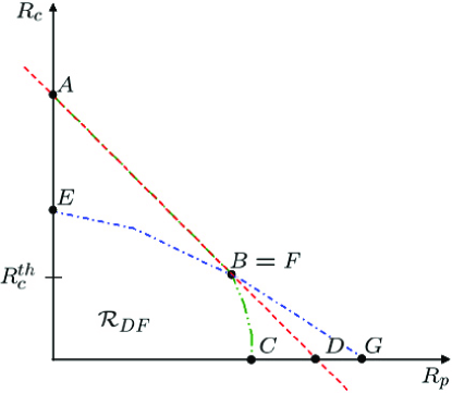
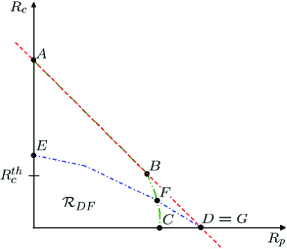
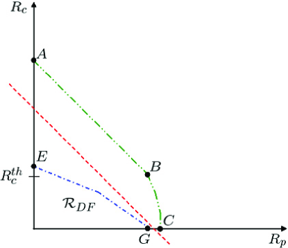
where DF=BC(Ps)MAC(Pr1,Pr2)subscript𝐷𝐹subscript𝐵𝐶subscript𝑃𝑠subscript𝑀𝐴𝐶subscript𝑃𝑟1subscript𝑃𝑟2\mathcal{R}_{DF}=\mathcal{R}_{BC}\left(P_{s}\right)\cap\mathcal{R}_{MAC}\left({P_{r1},P_{r2}}\right). Fig. 7. shows examples of the rate regions of MISO BC and SIMO MAC, the intersection of which is the achievable rate region by DF.

If the source-to-relay link SNR is high enough, the second hop becomes the bottleneck and determines the source-to-destination sum-rate.

Theorem 5 (Optimality condition of DF)

If there is a rate triple (R1,R2,Rc)sub(|ρ|opt)subscript𝑅1subscript𝑅2subscript𝑅𝑐subscript𝑠𝑢𝑏superscript𝜌𝑜𝑝𝑡\left(R_{1},R_{2},R_{c}\right)\in\mathcal{R}_{sub}\left({\left|\rho\right|^{opt}}\right) which is included in the MISO BC region BC(Ps)subscript𝐵𝐶subscript𝑃𝑠\mathcal{R}_{BC}\left(P_{s}\right), then RDFmax=Rsum,MACmaxsuperscriptsubscript𝑅𝐷𝐹𝑚𝑎𝑥superscriptsubscript𝑅𝑠𝑢𝑚𝑀𝐴𝐶𝑚𝑎𝑥R_{DF}^{max}=R_{sum,MAC}^{max} meets the upper bound and determines the capacity of the vector Gaussian parallel relay network.

Proof:

Let us first consider |ρ|opt=1superscript𝜌𝑜𝑝𝑡1|\rho|^{opt}=1 case where there is a single maximum sum-rate point in the SIMO MAC region. At |ρ|=1𝜌1|\rho|=1, the term logdet(𝐈+𝐇𝐐r𝐇)𝐈subscript𝐇𝐐𝑟superscript𝐇\log\det\left({\mathbf{I}+\mathbf{HQ}_{r}\mathbf{H}^{\dagger}}\right) in (2) and (3) is maximized and is smaller than (1) since the following relationships are hold:

Rsum,MACmaxRc,BCmaxRi,BCmax(i{1,2})Rsum,BCmaxRBCupper.superscriptsubscript𝑅𝑠𝑢𝑚𝑀𝐴𝐶𝑚𝑎𝑥superscriptsubscript𝑅𝑐𝐵𝐶𝑚𝑎𝑥superscriptsubscript𝑅𝑖𝐵𝐶𝑚𝑎𝑥𝑖12superscriptsubscript𝑅𝑠𝑢𝑚𝐵𝐶𝑚𝑎𝑥superscriptsubscript𝑅𝐵𝐶𝑢𝑝𝑝𝑒𝑟R_{sum,MAC}^{max}\leq R_{c,BC}^{max}\leq R_{i,BC}^{max}(i\in\{1,2\})\leq R_{sum,BC}^{max}\leq R_{BC}^{upper}.

We can achieve the tightest upper bound Rsum,MACmaxsuperscriptsubscript𝑅𝑠𝑢𝑚𝑀𝐴𝐶𝑚𝑎𝑥R_{sum,MAC}^{max} by allocating all relay power to the common signal: α=β=|γ|=1𝛼𝛽𝛾1\alpha=\beta=|\gamma|=1.

Now we consider |ρ|opt<1superscript𝜌𝑜𝑝𝑡1|\rho|^{opt}<1 case where there exist more than one maximum sum-rate point in the SIMO MAC region. It is tedious but easy to verify that, at |ρ|=|ρ|opt𝜌superscript𝜌𝑜𝑝𝑡|\rho|=|\rho|^{opt},

Rsum,MACmaxRsum,BCmaxRBCuppersuperscriptsubscript𝑅𝑠𝑢𝑚𝑀𝐴𝐶𝑚𝑎𝑥superscriptsubscript𝑅𝑠𝑢𝑚𝐵𝐶𝑚𝑎𝑥superscriptsubscript𝑅𝐵𝐶𝑢𝑝𝑝𝑒𝑟R_{sum,MAC}^{max}\leq R_{sum,BC}^{max}\leq R_{BC}^{upper}
2logdet(𝐈+𝐇𝐐r𝐇)i=1,2log(1+Ps𝐠i2)+i=1,2log(1+(1|ρ|2)Pri𝐡i2).2𝐈subscript𝐇𝐐𝑟superscript𝐇subscript𝑖121subscript𝑃𝑠superscriptnormsubscript𝐠𝑖2subscript𝑖1211superscript𝜌2subscript𝑃𝑟𝑖superscriptnormsubscript𝐡𝑖22\log\det\left({\mathbf{I}+\mathbf{HQ}_{r}\mathbf{H}^{\dagger}}\right)\leq\sum\limits_{i=1,2}\log({1+P_{s}\left\|{\mathbf{g}_{i}}\right\|^{2}})+\sum\limits_{i=1,2}\log\left(1+(1-|\rho|^{2})P_{ri}\left\|{\mathbf{h}_{i}}\right\|^{2}\right).

We can achieve the tightest upper bound Rsum,MACmaxsuperscriptsubscript𝑅𝑠𝑢𝑚𝑀𝐴𝐶𝑚𝑎𝑥R_{sum,MAC}^{max} by optimal power allocation at relays such that |ρ|opt=|γ|αβsuperscript𝜌𝑜𝑝𝑡𝛾𝛼𝛽|\rho|^{opt}=|\gamma|\sqrt{\alpha\beta}. ∎

With DF, the first and second hops are completely separated in the sense that after finishing the first stage of transmission, relays start a new stage of transmission by encoding the received information again. Here, the right approach is first to figure out what is optimal in the second hop, and then to check if the optimal operating point, i.e., one of the maximum sum-rate points of the SIMO MAC is supportable by the first hop. If the optimal point is achievable, the network nodes would start communication by setting parameters to satisfy optimality conditions. If none of the maximum sum-rate points of the SIMO MAC is achievable, then the nodes would try to find the operating point as close to the optimal as possible.

What if the relay-to-destination link SNRs are high enough so that the first hop is the bottleneck? If one of the maximum sum-rate points of the MISO BC on the R1R2subscript𝑅1subscript𝑅2R_{1}-R_{2} plane is included in MACsubscript𝑀𝐴𝐶\mathcal{R}_{MAC}, then RDFmax=Rsum,BCmaxsuperscriptsubscript𝑅𝐷𝐹𝑚𝑎𝑥superscriptsubscript𝑅𝑠𝑢𝑚𝐵𝐶𝑚𝑎𝑥R_{DF}^{max}=R_{sum,BC}^{max}. In this case, the broadcast cut-set upper bound in (1) is tighter than the others. It turns out that the upper bound and the achievable rate meet in some special cases where the first hop row vectors are orthogonal as will be seen in numerical results in Section VII. However, they do not meet in general, which implies suboptimality of DF in the case. If the first hop is the bottleneck, full decoding at relays gives too much restriction, and AF and CF schemes can do better.

IV-F Symmetric Channels

In this subsection, we narrow down our attention to the symmetric channels: 𝐠1=𝐠2normsubscript𝐠1normsubscript𝐠2\left\|{\mathbf{g}_{1}}\right\|=\left\|{\mathbf{g}_{2}}\right\|, 𝐡1=𝐡2normsubscript𝐡1normsubscript𝐡2\left\|{\mathbf{h}_{1}}\right\|=\left\|{\mathbf{h}_{2}}\right\|, Pr1=Pr2subscript𝑃𝑟1subscript𝑃𝑟2P_{r1}=P_{r2}, and R1=R2subscript𝑅1subscript𝑅2R_{1}=R_{2}. We consider four examples illustrated in Fig. 8. where Rp=R1+R2subscript𝑅𝑝subscript𝑅1subscript𝑅2R_{p}=R_{1}+R_{2}.

In Fig. 8. (a), the straight line AB¯¯𝐴𝐵\overline{AB} and the curved line BC¯¯𝐵𝐶\overline{BC} constitute the surface of the MAC achievable rate region. The curved line EG¯¯𝐸𝐺\overline{EG} is the surface of the BC achievable rate region. Here, we have the source power constraint Pssubscript𝑃𝑠P_{s} so large that the upper bound (1) and the second terms of min𝑚𝑖𝑛min in (2) and (3) are loose. In this case, logdet(𝐈+𝐇𝐐r𝐇)𝐈subscript𝐇𝐐𝑟superscript𝐇\log\det\left({\mathbf{I}+\mathbf{HQ}_{r}\mathbf{H}^{\dagger}}\right) is the active upper bound, and the sum-rate constraint R1+R2+Rcsubscript𝑅1subscript𝑅2subscript𝑅𝑐R_{1}+R_{2}+R_{c} is the straight line that goes through the points A𝐴A, B𝐵B, and D𝐷D. The straight line AB¯¯𝐴𝐵\overline{AB} is the maximum sum-rate subregion of the MAC, and F𝐹F is the crossing point of the BC and MAC surfaces. All the points on the line FB¯¯𝐹𝐵\overline{FB} achieve the capacity of the vector Gaussian parallel relay network as they are in the BC and MAC achievable rate regions and meet the sum-rate upper bound.

Other things being equal, the BC rate region with a smaller power constraint is drawn in Fig. 8. (b). In this example, the crossing point F𝐹F coincides with the point B𝐵B. Thus, there exists a single capacity achieving point at B=F𝐵𝐹B=F. In Fig. 8. (c), the BC rate region gets even smaller, and the DF maximum sum-rate point F𝐹F does not meet the sum-rate upper bound. Thus, in this case, DF does not achieve the capacity of the vector Gaussian parallel relay network. Finally, Fig. 8. (d) illustrates the case where the source power constraint Pssubscript𝑃𝑠P_{s} is so small that logdet(𝐈+𝐇𝐐r𝐇)𝐈subscript𝐇𝐐𝑟superscript𝐇\log\det\left({\mathbf{I}+\mathbf{HQ}_{r}\mathbf{H}^{\dagger}}\right) in the upper bound expression is not active anymore.

V Amplify-and-Forward (AF)

We have seen that if the relay-to-destination link SNR is high enough, the first hop is the bottleneck and DF does not satisfy the optimality condition that requires at least one maximum sum-rate point of SIMO MAC should be inside MISO BC achievable region. Instead of requiring signals with low SNR to be decoded at relays, it would be better for relays to just forward their received signals to the destination so that the benefit of high SNR in the second hop is maximally utilized.

V-A Achievable Rate of AF

The received signal at relays can be expressed in vector notation by

𝐲r=𝐆𝐱s+𝐧r.subscript𝐲𝑟subscript𝐆𝐱𝑠subscript𝐧𝑟\mathbf{y}_{r}=\mathbf{Gx}_{s}+\mathbf{n}_{r}.

With AF, the relays just amplify their received signals before forwarding them to the destination, and the transmit signal vector of the relays is given by

𝐱r=𝐀𝐲rsubscript𝐱𝑟subscript𝐀𝐲𝑟\mathbf{x}_{r}=\mathbf{Ay}_{r}

where 𝐀=diag[aejϕ,b]𝐀𝑑𝑖𝑎𝑔𝑎superscript𝑒𝑗italic-ϕ𝑏\mathbf{A}=diag[ae^{j\phi},b]. The amplification factors should be in the range

0aapeak=Pr11+𝐠1𝐐s𝐠1, 0bbpeak=Pr21+𝐠2𝐐s𝐠2formulae-sequence0𝑎superscript𝑎𝑝𝑒𝑎𝑘subscript𝑃𝑟11subscript𝐠1subscript𝐐𝑠superscriptsubscript𝐠1 0𝑏superscript𝑏𝑝𝑒𝑎𝑘subscript𝑃𝑟21subscript𝐠2subscript𝐐𝑠superscriptsubscript𝐠20\leq a\leq a^{peak}=\sqrt{\frac{{P_{r1}}}{{1+\mathbf{g}_{1}\mathbf{Q}_{s}\mathbf{g}_{1}^{{\dagger}}}}},\ \ 0\leq b\leq b^{peak}=\sqrt{\frac{{P_{r2}}}{{1+\mathbf{g}_{2}\mathbf{Q}_{s}\mathbf{g}_{2}^{{\dagger}}}}}

because of the power constraints at the relays. The received signal at the destination is given by

𝐲d=𝐇𝐱r+𝐧d=𝐇𝐀𝐲r+𝐧d=𝐇𝐀𝐆𝐱s+𝐇𝐀𝐧r+𝐧d=𝐇𝐀𝐆𝐱s+𝐧e=(aejϕ𝐡1𝐠1+b𝐡2𝐠2)𝐱s+(aejϕnr1𝐡1+bnr2𝐡2+𝐧d)subscript𝐲𝑑subscript𝐇𝐱𝑟subscript𝐧𝑑subscript𝐇𝐀𝐲𝑟subscript𝐧𝑑subscript𝐇𝐀𝐆𝐱𝑠subscript𝐇𝐀𝐧𝑟subscript𝐧𝑑subscript𝐇𝐀𝐆𝐱𝑠subscript𝐧𝑒𝑎superscript𝑒𝑗italic-ϕsubscript𝐡1subscript𝐠1𝑏subscript𝐡2subscript𝐠2subscript𝐱𝑠𝑎superscript𝑒𝑗italic-ϕsubscript𝑛𝑟1subscript𝐡1𝑏subscript𝑛𝑟2subscript𝐡2subscript𝐧𝑑\begin{gathered}\mathbf{y}_{d}=\mathbf{Hx}_{r}+\mathbf{n}_{d}=\mathbf{HAy}_{r}+\mathbf{n}_{d}\hfill\\ =\mathbf{HAGx}_{s}+\mathbf{HAn}_{r}+\mathbf{n}_{d}\hfill\\ =\mathbf{HAGx}_{s}+\mathbf{n}_{e}\hfill\\ =(ae^{j\phi}\mathbf{h}_{1}\mathbf{g}_{1}+b\mathbf{h}_{2}\mathbf{g}_{2})\mathbf{x}_{s}+(ae^{j\phi}n_{r1}\mathbf{h}_{1}+bn_{r2}\mathbf{h}_{2}+\mathbf{n}_{d})\end{gathered}

where 𝐧esubscript𝐧𝑒{\bf n}_{e} denotes the total effective noise. Since the noises added at relay receivers are also amplified and forwarded through the channel, the noise vector 𝐧esubscript𝐧𝑒{\bf n}_{e} is spatially non-white in general. Noise covariance matrix is symmetric and can be decomposed as

𝐊=𝔼[𝐧e𝐧e]=𝐈+𝐇𝐀𝐀𝐇=𝐔𝚲𝐔𝐊𝔼delimited-[]subscript𝐧𝑒superscriptsubscript𝐧𝑒𝐈superscript𝐇𝐀𝐀superscript𝐇superscript𝐔𝚲𝐔\mathbf{K}=\mathbb{E}[\mathbf{n}_{e}\mathbf{n}_{e}^{{\dagger}}]=\mathbf{I+HAA^{\dagger}H^{\dagger}}=\mathbf{U^{\dagger}\Lambda U}

where ΛΛ\Lambda is a diagonal matrix with eigenvalues of 𝐊𝐊\bf K as its diagonal elements, and 𝐔𝐔\bf U is a unitary matrix. Then, the channel can be transformed into an equivalent white noise channel given by

𝚲1/2𝐔𝐲d=𝚲1/2𝐔𝐇𝐀𝐆𝐱s+𝚲1/2𝐔𝐧e=𝐅𝐱s+𝐧wsuperscript𝚲12subscript𝐔𝐲𝑑superscript𝚲12subscript𝐔𝐇𝐀𝐆𝐱𝑠superscript𝚲12subscript𝐔𝐧𝑒subscript𝐅𝐱𝑠subscript𝐧𝑤\mathbf{\Lambda}^{-1/2}\mathbf{Uy}_{d}=\mathbf{\Lambda}^{-1/2}\mathbf{UHAGx}_{s}+\mathbf{\Lambda}^{-1/2}\mathbf{Un}_{e}\hfill\\ =\mathbf{Fx}_{s}+\mathbf{n}_{w}

where 𝐅𝐅\bf F and 𝐧wsubscript𝐧𝑤{\bf n}_{w} denote the effective source-to-destination channel matrix and the white noise vector, respectively. For a fixed 𝐀𝐀\bf A, this is a point-to-point MIMO channel whose maximum rank is 222 limited by the number of relays. If all the input signal is Gaussian, we get the expression for an achievable rate by AF given by

RAFI(𝐱s;𝐲d)=logdet(𝐈+𝐇𝐀𝐀𝐇+𝐇𝐀𝐆𝐐s𝐆𝐀𝐇)det(𝐈+𝐇𝐀𝐀𝐇)=logdet(𝐈+𝚲1/2𝐔𝐇𝐀𝐆𝐐s𝐆𝐀𝐇𝐔𝚲1/2)=logdet(𝐈+𝐅𝐐s𝐅).subscript𝑅𝐴𝐹𝐼subscript𝐱𝑠subscript𝐲𝑑𝐈superscript𝐇𝐀𝐀superscript𝐇subscript𝐇𝐀𝐆𝐐𝑠superscript𝐆superscript𝐀superscript𝐇𝐈superscript𝐇𝐀𝐀superscript𝐇𝐈superscript𝚲12subscript𝐔𝐇𝐀𝐆𝐐𝑠superscript𝐆superscript𝐀superscript𝐇superscript𝐔superscript𝚲12𝐈subscript𝐅𝐐𝑠superscript𝐅\displaystyle\begin{gathered}R_{AF}\leq I(\mathbf{x}_{s};\mathbf{y}_{d})\hfill\\ =\log\frac{{\det\left({\mathbf{I}+\mathbf{HAA}^{{\dagger}}\mathbf{H}^{{\dagger}}+\mathbf{HAGQ}_{s}\mathbf{G}^{{\dagger}}\mathbf{A}^{{\dagger}}\mathbf{H}^{{\dagger}}}\right)}}{{\det\left({\mathbf{I}+\mathbf{HAA}^{{\dagger}}\mathbf{H}^{{\dagger}}}\right)}}\hfill\\ =\log\det\left({\mathbf{I}+\mathbf{\Lambda}^{-1/2}\mathbf{UHAGQ}_{s}\mathbf{G}^{{\dagger}}\mathbf{A}^{{\dagger}}\mathbf{H}^{{\dagger}}\mathbf{U}^{{\dagger}}\mathbf{\Lambda}^{-1/2}}\right)\hfill\\ =\log\det\left({\mathbf{I}+\mathbf{FQ}_{s}\mathbf{F}^{{\dagger}}}\right).\hfill\end{gathered} (43)

In order to get the maximum achievable rate, the source signal covariance matrix 𝐐ssubscript𝐐𝑠\mathbf{Q}_{s} and the relay amplification matrix 𝐀𝐀\bf A need to be jointly optimized.

Theorem 6 (Asymptotic Optimality of AF)

If 𝐇𝐇\bf H is full rank, AF is asymptotically optimal in the high relay power limit in the sense that

limPr1=Pr2(max𝐐slogdet(𝐈+𝐆𝐐s𝐆)max𝐐s,𝐀RAF)=0.subscriptsubscript𝑃𝑟1subscript𝑃𝑟2subscriptsubscript𝐐𝑠𝐈subscript𝐆𝐐𝑠superscript𝐆subscriptsubscript𝐐𝑠𝐀subscript𝑅𝐴𝐹0\mathop{\lim}\limits_{P_{r1}=P_{r2}\to\infty}(\mathop{\max}\limits_{\mathbf{Q}_{s}}\log\det\left({\mathbf{I}+\mathbf{GQ}_{s}\mathbf{G}^{{\dagger}}}\right)-\mathop{\max}\limits_{\mathbf{Q}_{s},\mathbf{A}}R_{AF})=0.

Proof:

By rearranging (43), we get

RAF=logdet(𝐈+𝐇𝐀𝐆𝐐s𝐆𝐀𝐇(𝐈+𝐇𝐀𝐀𝐇)𝟏)=logdet(𝐈+𝐆𝐐s𝐆𝐀𝐇(𝐈+𝐇𝐀𝐀𝐇)𝟏𝐇𝐀)=logdet(𝐈+𝐆𝐐s𝐆(𝐈(𝐈+𝐀𝐇𝐇𝐀)𝟏))subscript𝑅𝐴𝐹𝐈subscript𝐇𝐀𝐆𝐐𝑠superscript𝐆superscript𝐀superscript𝐇superscript𝐈superscript𝐇𝐀𝐀superscript𝐇1𝐈subscript𝐆𝐐𝑠superscript𝐆superscript𝐀superscript𝐇superscript𝐈superscript𝐇𝐀𝐀superscript𝐇1𝐇𝐀𝐈subscript𝐆𝐐𝑠superscript𝐆𝐈superscript𝐈superscript𝐀superscript𝐇𝐇𝐀1\begin{gathered}R_{AF}=\log\det\left(\mathbf{I+HAGQ}_{s}\mathbf{G^{\dagger}A^{\dagger}H^{\dagger}\left({I+HAA^{\dagger}H^{\dagger}}\right)^{-1}}\right)\hfill\\ =\log\det\left(\mathbf{I+GQ}_{s}\mathbf{G^{\dagger}A^{\dagger}H^{\dagger}\left({I+HAA^{\dagger}H^{\dagger}}\right)^{-1}HA}\right)\hfill\\ =\log\det\left(\mathbf{I+GQ}_{s}\mathbf{G^{\dagger}\left({I-\left({I+A^{\dagger}H^{\dagger}HA}\right)^{-1}}\right)}\right)\hfill\\ \end{gathered}

where we use matrix inversion lemma. We first set a𝑎a and b𝑏b to peak values under relay power constraints, assume ϕitalic-ϕ\phi is optimally chosen, and let RAFpeaksuperscriptsubscript𝑅𝐴𝐹𝑝𝑒𝑎𝑘R_{AF}^{peak} denote the corresponding rate. By showing that if det(𝐇𝐇)>0superscript𝐇𝐇0\det(\mathbf{H}^{\mathbf{{\dagger}}}\mathbf{H})>0, (𝐈+𝐀𝐇𝐇𝐀)1𝟎superscript𝐈superscript𝐀superscript𝐇𝐇𝐀10\left(\mathbf{I+A^{\dagger}H^{\dagger}HA}\right)^{-1}\to\mathbf{0} as a𝑎a\to\infty and b𝑏b\to\infty where

(𝐈+𝐀𝐇𝐇𝐀)1=[1+b2𝐡22abejϕ𝐡1𝐡2abejϕ𝐡2𝐡11+a2𝐡12]1+a2𝐡12+b2𝐡22+a2b2det(𝐇𝐇),superscript𝐈superscript𝐀superscript𝐇𝐇𝐀1delimited-[]1superscript𝑏2superscriptnormsubscript𝐡22𝑎𝑏superscript𝑒𝑗italic-ϕsuperscriptsubscript𝐡1subscript𝐡2missing-subexpressionmissing-subexpressionmissing-subexpressionmissing-subexpressionmissing-subexpressionmissing-subexpressionmissing-subexpressionmissing-subexpressionmissing-subexpressionmissing-subexpressionmissing-subexpressionmissing-subexpressionmissing-subexpressionmissing-subexpressionmissing-subexpressionmissing-subexpressionmissing-subexpressionmissing-subexpression𝑎𝑏superscript𝑒𝑗italic-ϕsuperscriptsubscript𝐡2subscript𝐡11superscript𝑎2superscriptnormsubscript𝐡12missing-subexpressionmissing-subexpressionmissing-subexpressionmissing-subexpressionmissing-subexpressionmissing-subexpressionmissing-subexpressionmissing-subexpressionmissing-subexpressionmissing-subexpressionmissing-subexpressionmissing-subexpressionmissing-subexpressionmissing-subexpressionmissing-subexpressionmissing-subexpressionmissing-subexpressionmissing-subexpression1superscript𝑎2superscriptnormsubscript𝐡12superscript𝑏2superscriptnormsubscript𝐡22superscript𝑎2superscript𝑏2superscript𝐇𝐇\left(\mathbf{I+A^{\dagger}H^{\dagger}HA}\right)^{-1}=\frac{{\left[{\begin{array}[]{*{20}c}{1+b^{2}\left\|{\mathbf{h}_{2}}\right\|^{2}}&{-abe^{-j\phi}\mathbf{h}_{1}^{\mathbf{{\dagger}}}\mathbf{h}_{2}}\\ {-abe^{j\phi}\mathbf{h}_{2}^{\mathbf{{\dagger}}}\mathbf{h}_{1}}&{1+a^{2}\left\|{\mathbf{h}_{1}}\right\|^{2}}\\ \end{array}}\right]}}{{1+a^{2}\left\|{\mathbf{h}_{1}}\right\|^{2}+b^{2}\left\|{\mathbf{h}_{2}}\right\|^{2}+a^{2}b^{2}\det(\mathbf{H}^{\mathbf{{\dagger}}}\mathbf{H})}},

we get the following result

limPr1=Pr2(logdet(𝐈+𝐆𝐐s𝐆)RAFpeak)=0subscriptsubscript𝑃𝑟1subscript𝑃𝑟2𝐈subscript𝐆𝐐𝑠superscript𝐆superscriptsubscript𝑅𝐴𝐹𝑝𝑒𝑎𝑘0\mathop{\lim}\limits_{P_{r1}=P_{r2}\to\infty}\left(\log\det\left({\mathbf{I}+\mathbf{GQ}_{s}\mathbf{G}^{\mathbf{{\dagger}}}}\right)-R_{AF}^{peak}\right)=0

Then, the theorem statement naturally follows since by definition, for a fixed 𝐐ssubscript𝐐𝑠{\bf Q}_{s},

RAFpeakmax𝐀RAF.superscriptsubscript𝑅𝐴𝐹𝑝𝑒𝑎𝑘subscript𝐀subscript𝑅𝐴𝐹R_{AF}^{peak}\leq\mathop{\max}\limits_{\mathbf{A}}R_{AF}.

V-B Iterative Optimization Algorithm for AF

We can maximize RAFsubscript𝑅𝐴𝐹R_{AF} by an iterative algorithm as follows. For optimizing 𝐐ssubscript𝐐𝑠\mathbf{Q}_{s}, we apply singular value decomposition (SVD) to 𝐅𝐅\bf F and waterfilling over two parallel scalar channels with non-zero singular values [19]. First, we define the covariance matrix of 𝐆𝐱ssubscript𝐆𝐱𝑠{\bf Gx}_{s} and the rate function of (a,b)𝑎𝑏(a,b) given by

𝐐e=𝔼[𝐆𝐱s𝐱s𝐆]=𝐆𝐐𝐬𝐆=[q11q12q21q22],superscript𝐐𝑒𝔼delimited-[]subscript𝐆𝐱𝑠superscriptsubscript𝐱𝑠superscript𝐆subscript𝐆𝐐𝐬superscript𝐆delimited-[]subscript𝑞11subscript𝑞12missing-subexpressionmissing-subexpressionmissing-subexpressionmissing-subexpressionmissing-subexpressionmissing-subexpressionmissing-subexpressionmissing-subexpressionmissing-subexpressionmissing-subexpressionmissing-subexpressionmissing-subexpressionmissing-subexpressionmissing-subexpressionmissing-subexpressionmissing-subexpressionmissing-subexpressionmissing-subexpressionsubscript𝑞21subscript𝑞22missing-subexpressionmissing-subexpressionmissing-subexpressionmissing-subexpressionmissing-subexpressionmissing-subexpressionmissing-subexpressionmissing-subexpressionmissing-subexpressionmissing-subexpressionmissing-subexpressionmissing-subexpressionmissing-subexpressionmissing-subexpressionmissing-subexpressionmissing-subexpressionmissing-subexpressionmissing-subexpression\mathbf{Q}^{e}=\mathbb{E}[{\bf Gx}_{s}{\bf x}_{s}^{\dagger}{\bf G}^{\dagger}]=\mathbf{GQ_{s}G^{\dagger}}=\left[{\begin{array}[]{*{20}c}{q_{11}}&{q_{12}}\\ {q_{21}}&{q_{22}}\\ \end{array}}\right],
R(a,b)=log(1+a2b2det(𝐇𝐇)(tr(𝐐e)+det(𝐐e))+a2𝐡12q11+b2𝐡22q22+2aejϕb𝐡1𝐡2q211+a2𝐡12+b2𝐡22+a2b2det(𝐇𝐇)).𝑅𝑎𝑏1superscript𝑎2superscript𝑏2superscript𝐇𝐇trsuperscript𝐐𝑒superscript𝐐𝑒superscript𝑎2superscriptnormsubscript𝐡12subscript𝑞11superscript𝑏2superscriptnormsubscript𝐡22subscript𝑞222𝑎superscript𝑒𝑗italic-ϕ𝑏superscriptsubscript𝐡1subscript𝐡2subscript𝑞211superscript𝑎2superscriptnormsubscript𝐡12superscript𝑏2superscriptnormsubscript𝐡22superscript𝑎2superscript𝑏2superscript𝐇𝐇\begin{gathered}R(a,b)=\hfill\\ \log\left({1+\frac{{a^{2}b^{2}\det(\mathbf{H}^{{\dagger}}\mathbf{H})(\text{tr}(\mathbf{Q}^{e})+\det(\mathbf{Q}^{e}))+a^{2}\left\|{\mathbf{h}_{1}}\right\|^{2}q_{11}+b^{2}\left\|{\mathbf{h}_{2}}\right\|^{2}q_{22}+2ae^{-j\phi}b{\mathbf{h}_{1}^{{\dagger}}\mathbf{h}_{2}q_{21}}}}{{1+a^{2}\left\|{\mathbf{h}_{1}}\right\|^{2}+b^{2}\left\|{\mathbf{h}_{2}}\right\|^{2}+a^{2}b^{2}\det(\mathbf{H}^{{\dagger}}\mathbf{H})}}}\right).\end{gathered}

  
Next, we do the following steps:

Step 0) Set 𝐐s=diag[Ps/2,Ps/2]subscript𝐐𝑠𝑑𝑖𝑎𝑔subscript𝑃𝑠2subscript𝑃𝑠2\mathbf{Q}_{s}=diag[P_{s}/2,P_{s}/2].

Step 1) Calculate 𝐐e=𝐆𝐐s𝐆superscript𝐐𝑒subscript𝐆𝐐𝑠superscript𝐆\mathbf{Q}^{e}=\mathbf{GQ}_{s}\mathbf{G}^{\dagger}.
                                Set apeak=Pr11+q11superscript𝑎𝑝𝑒𝑎𝑘subscript𝑃𝑟11subscript𝑞11a^{peak}=\sqrt{\frac{{P_{r1}}}{{1+q_{11}}}}, bpeak=Pr21+q22superscript𝑏𝑝𝑒𝑎𝑘subscript𝑃𝑟21subscript𝑞22b^{peak}=\sqrt{\frac{{P_{r2}}}{{1+q_{22}}}}, and ϕ=(𝐡1𝐡2q21)italic-ϕsuperscriptsubscript𝐡1subscript𝐡2subscript𝑞21\phi=\angle(\mathbf{h}_{1}^{{\dagger}}\mathbf{h}_{2}q_{21}).

Step 2) Calculate maxaR(a,bpeak)subscript𝑎𝑅𝑎superscript𝑏𝑝𝑒𝑎𝑘\mathop{\max}\limits_{a}R(a,b^{peak}) subject to 0aapeak0𝑎superscript𝑎𝑝𝑒𝑎𝑘0\leq a\leq a^{peak} by solving aR(a,bpeak)=0𝑎𝑅𝑎superscript𝑏𝑝𝑒𝑎𝑘0\frac{\partial}{{\partial a}}R(a,b^{peak})=0.
                                Calculate maxbR(apeak,b)subscript𝑏𝑅superscript𝑎𝑝𝑒𝑎𝑘𝑏\mathop{\max}\limits_{b}R(a^{peak},b) subject to 0bbpeak0𝑏superscript𝑏𝑝𝑒𝑎𝑘0\leq b\leq b^{peak} by solving bR(apeak,b)=0𝑏𝑅superscript𝑎𝑝𝑒𝑎𝑘𝑏0\frac{\partial}{{\partial b}}R(a^{peak},b)=0.
                  Between (aopt,bpeak)superscript𝑎𝑜𝑝𝑡superscript𝑏𝑝𝑒𝑎𝑘(a^{opt},b^{peak}) and (apeak,bopt)superscript𝑎𝑝𝑒𝑎𝑘superscript𝑏𝑜𝑝𝑡(a^{peak},b^{opt}), choose the one that results in a higher rate.

Step 3) Set 𝐀=diag[aejϕ,b]𝐀𝑑𝑖𝑎𝑔𝑎superscript𝑒𝑗italic-ϕ𝑏{\bf A}=diag[ae^{j\phi},b] using the values obtained above.
                                Calculate 𝐊𝐊\mathbf{K} and do eigenvalue decomposition to get 𝐔𝐔\bf U and ΛΛ\Lambda such that

𝐊=𝐈+𝐇𝐀𝐀𝐇=𝐔𝚲𝐔.𝐊𝐈superscript𝐇𝐀𝐀superscript𝐇superscript𝐔𝚲𝐔\mathbf{K=I+HAA^{\dagger}H^{\dagger}=U^{\dagger}\Lambda U}.

                                Calculate 𝐅=𝚲1/2𝐔𝐇𝐀𝐆𝐅superscript𝚲12𝐔𝐇𝐀𝐆{\bf F}=\mathbf{\Lambda}^{-1/2}\mathbf{UHAG}.

Step 4) Optimize 𝐐ssubscript𝐐𝑠\mathbf{Q}_{s} via singular value decomposition of 𝐅𝐅\bf F and waterfilling [19].
                                Update 𝐐ssubscript𝐐𝑠\mathbf{Q}_{s} and calculate RAF=logdet(𝐈+𝐅𝐐s𝐅)subscript𝑅𝐴𝐹𝐈subscript𝐅𝐐𝑠superscript𝐅R_{AF}=\log\det\left({\mathbf{I+FQ}_{s}\mathbf{F^{\dagger}}}\right).

Step 5) Terminate if RAFsubscript𝑅𝐴𝐹R_{AF} already converged to a certain value.
                                Otherwise, go to Step 1.

Before closing the section, it is worth noting that full power transmission sometimes hurts. This is the case when one of the relays has received a signal with very low SNR so that transmission at full power degrades the received SNR at the destination. Fig. 9 shows examples. For each of the two different values of 𝐠2normsubscript𝐠2\left\|{\bf g}_{2}\right\| shown in the figure, we run the algorithm steps from 0 to 4 just once, and draw the resulting R(apeak,b)𝑅superscript𝑎𝑝𝑒𝑎𝑘𝑏R(a^{peak},b) versus b𝑏b curves. For the curve in Fiq. 9. (a), the maximum of the curve indicated by a circle happens at a point of b𝑏b above bpeaksuperscript𝑏𝑝𝑒𝑎𝑘b^{peak} indicated by vertical line. It means that the received SNR at the second relay is still high, and full power transmission helps. However, for the curve in Fiq. 9. (b), as the maximum happens at a point less than bpeaksuperscript𝑏𝑝𝑒𝑎𝑘b^{peak}, the received SNR at the second relay is too low for transmission at full power to be optimal.

VI Compress-and-Forward (CF)

For CF, relays compress or quantize their received signals, re-encode, and forward them to the destination. At the destination, the decoder tries to decode the received signal to recover relay input signals, and finally decompress the relay signals to recover the information transmitted from the source. CF achievable rates were first derived by applying Wyner-Ziv source coding [15] to a classical one relay model in [3], their extension to multiple relay models in [4]. The derivation for a special case of the Gaussian parallel relay network with N=M=1𝑁𝑀1N=M=1 can be found in [1] and [2]. The extension to our network model in terms of mutual information is straightforward as follows

RCFI(𝐱s;y^r1,y^r2)I(y^r1;yr1|y^r2)I(xr1;𝐲d|xr2)I(y^r2;yr2|y^r1)I(xr2;𝐲d|xr1)I(y^r1,y^r2;yr1,yr2)I(xr1,xr2;𝐲d).subscript𝑅𝐶𝐹𝐼subscript𝐱𝑠subscript^𝑦𝑟1subscript^𝑦𝑟2𝐼subscript^𝑦𝑟1conditionalsubscript𝑦𝑟1subscript^𝑦𝑟2𝐼subscript𝑥𝑟1conditionalsubscript𝐲𝑑subscript𝑥𝑟2𝐼subscript^𝑦𝑟2conditionalsubscript𝑦𝑟2subscript^𝑦𝑟1𝐼subscript𝑥𝑟2conditionalsubscript𝐲𝑑subscript𝑥𝑟1𝐼subscript^𝑦𝑟1subscript^𝑦𝑟2subscript𝑦𝑟1subscript𝑦𝑟2𝐼subscript𝑥𝑟1subscript𝑥𝑟2subscript𝐲𝑑\displaystyle\begin{gathered}R_{CF}\leq I(\mathbf{x}_{s};\hat{y}_{r1},\hat{y}_{r2})\hfill\\ I(\hat{y}_{r1};y_{r1}|\hat{y}_{r2})\leq I(x_{r1};\mathbf{y}_{d}|x_{r2})\hfill\\ I(\hat{y}_{r2};y_{r2}|\hat{y}_{r1})\leq I(x_{r2};\mathbf{y}_{d}|x_{r1})\hfill\\ I(\hat{y}_{r1},\hat{y}_{r2};y_{r1},y_{r2})\leq I(x_{r1},x_{r2};\mathbf{y}_{d}).\hfill\\ \end{gathered} (49)

By introducing quantization noise, we have a compressed version of relay signals given by

y^r1=yr1+an^r1y^r2=yr2+bn^r2subscript^𝑦𝑟1subscript𝑦𝑟1𝑎subscript^𝑛𝑟1subscript^𝑦𝑟2subscript𝑦𝑟2𝑏subscript^𝑛𝑟2\displaystyle\begin{gathered}\hat{y}_{r1}=y_{r1}+\sqrt{a}\hat{n}_{r1}\hfill\\ \hat{y}_{r2}=y_{r2}+\sqrt{b}\hat{n}_{r2}\hfill\\ \end{gathered} (53)

where a,b>0𝑎𝑏0a,b>0. Assuming the quantization noise and all input signals are Gaussian distributed, we can evaluate the mutual information expressions to have the following result.

Theorem 7

With CF, the following rate is achievable in the vector Gaussian parallel relay network.

RCF=max𝐐s,𝐀logdet(𝐈+𝐀+𝐆𝐐s𝐆)(1+a)(1+b),subject to logdet(𝐈+𝐀+𝐆𝐐s𝐆)a(1+b+𝐠2𝐐s𝐠2)log(1+Pr1𝐡12), logdet(𝐈+𝐀+𝐆𝐐s𝐆)b(1+a+𝐠1𝐐s𝐠1)log(1+Pr2𝐡22), logdet(𝐈+𝐀+𝐆𝐐s𝐆)ablogdet(𝐈+𝐇𝐐r𝐇), tr(𝐐s)Ps, a,b0formulae-sequencesubscript𝑅𝐶𝐹subscriptsubscript𝐐𝑠𝐀𝐈𝐀subscript𝐆𝐐𝑠superscript𝐆1𝑎1𝑏formulae-sequencesubject to 𝐈𝐀subscript𝐆𝐐𝑠superscript𝐆𝑎1𝑏subscript𝐠2subscript𝐐𝑠superscriptsubscript𝐠21subscript𝑃𝑟1superscriptdelimited-∥∥subscript𝐡12formulae-sequence 𝐈𝐀subscript𝐆𝐐𝑠superscript𝐆𝑏1𝑎subscript𝐠1subscript𝐐𝑠superscriptsubscript𝐠11subscript𝑃𝑟2superscriptdelimited-∥∥subscript𝐡22formulae-sequence 𝐈𝐀subscript𝐆𝐐𝑠superscript𝐆𝑎𝑏𝐈subscript𝐇𝐐𝑟superscript𝐇formulae-sequence trsubscript𝐐𝑠subscript𝑃𝑠 𝑎𝑏0\displaystyle\begin{gathered}R_{CF}=\mathop{\max}\limits_{\mathbf{Q}_{s},\mathbf{A}}\log\frac{{\det\left({\mathbf{I}+\mathbf{A}+\mathbf{GQ}_{s}\mathbf{G}^{{\dagger}}}\right)}}{{(1+a)(1+b)}},\hfill\\ \mbox{subject to }\log\frac{{\det\left({\mathbf{I}+\mathbf{A}+\mathbf{GQ}_{s}\mathbf{G}^{{\dagger}}}\right)}}{{a(1+b+\mathbf{g}_{2}\mathbf{Q}_{s}\mathbf{g}_{2}^{\dagger})}}\leq\log(1+P_{r1}\left\|{\mathbf{h}_{1}}\right\|^{2}),\hfill\\ \mbox{\ \ \ \ \ \ \ \ \ \ \ \ }\log\frac{{\det\left({\mathbf{I}+\mathbf{A}+\mathbf{GQ}_{s}\mathbf{G}^{{\dagger}}}\right)}}{{b(1+a+\mathbf{g}_{1}\mathbf{Q}_{s}\mathbf{g}_{1}^{\dagger})}}\leq\log(1+P_{r2}\left\|{\mathbf{h}_{2}}\right\|^{2}),\hfill\\ \mbox{\ \ \ \ \ \ \ \ \ \ \ \ }\log\frac{{\det\left({\mathbf{I}+\mathbf{A}+\mathbf{GQ}_{s}\mathbf{G}^{{\dagger}}}\right)}}{{ab}}\leq\log\det\left({\mathbf{I}+\mathbf{HQ}_{r}\mathbf{H}^{{\dagger}}}\right),\hfill\\ \mbox{\ \ \ \ \ \ \ \ \ \ \ \ \ \ \ \ \ \ \ \ \ \ \ \ \ \ \ \ \ \ \ \ \ \ \ \ }{\rm tr}\left({{\bf Q}_{s}}\right)\leq P_{s},\hfill\\ \mbox{\ \ \ \ \ \ \ \ \ \ \ \ \ \ \ \ \ \ \ \ \ \ \ \ \ \ \ \ \ \ \ \ \ \ \ \ \ \ \ \ }a,b\geq 0\hfill\\ \end{gathered} (61)

where 𝐐s=𝔼[𝐱s𝐱s]subscript𝐐𝑠𝔼delimited-[]subscript𝐱𝑠superscriptsubscript𝐱𝑠\mathbf{Q}_{s}=\mathbb{E}[\mathbf{x}_{s}\mathbf{x}_{s}^{\dagger}], 𝐐r=𝔼[𝐱r𝐱r]=diag[Pr1,Pr2]subscript𝐐𝑟𝔼delimited-[]subscript𝐱𝑟superscriptsubscript𝐱𝑟𝑑𝑖𝑎𝑔subscript𝑃𝑟1subscript𝑃𝑟2\mathbf{Q}_{r}=\mathbb{E}[\mathbf{x}_{r}\mathbf{x}_{r}^{\dagger}]=diag[P_{r1},P_{r2}], and 𝐀=diag[a,b]𝐀𝑑𝑖𝑎𝑔𝑎𝑏\mathbf{A}=diag[a,b].

Proof:

It is straightforward to show the theorem result by evaluating the mutual information expressions with the assumption that the input distributions are circularly symmetric complex Gaussian. ∎

Similar to the AF scheme, the CF achievable rate becomes close to the upper bound as the relay power goes to infinity. We get the following result for the CF achievable rate.

Theorem 8 (Asymptotic Optimality of CF)

In the vector Gaussian parallel relay network, regardless of the rank of 𝐇𝐇\bf H, CF is asymptotically optimal in the high relay power limit in the sense that

limPr1=Pr2(max𝐐slogdet(𝐈+𝐆𝐐s𝐆)RCF)=0.subscriptsubscript𝑃𝑟1subscript𝑃𝑟2subscriptsubscript𝐐𝑠𝐈subscript𝐆𝐐𝑠superscript𝐆subscript𝑅𝐶𝐹0\mathop{\lim}\limits_{P_{r1}=P_{r2}\to\infty}(\mathop{\max}\limits_{\mathbf{Q}_{s}}\log\det\left({\mathbf{I}+\mathbf{GQ}_{s}\mathbf{G}^{{\dagger}}}\right)-R_{CF})=0.

Proof:

As Pr1subscript𝑃𝑟1P_{r1} and Pr2subscript𝑃𝑟2P_{r2} go to infinity, the optimization of RCFsubscript𝑅𝐶𝐹R_{CF} becomes unconstrained. The objective is maximum when a=b=0𝑎𝑏0a=b=0. Thus,

max𝐐s,𝐀logdet(𝐈+𝐆𝐐s𝐆(𝐈+𝐀)1)max𝐐slogdet(𝐈+𝐆𝐐s𝐆).subscriptsubscript𝐐𝑠𝐀𝐈subscript𝐆𝐐𝑠superscript𝐆superscript𝐈𝐀1subscriptsubscript𝐐𝑠𝐈subscript𝐆𝐐𝑠superscript𝐆\displaystyle\begin{gathered}\mathop{\max}\limits_{\mathbf{Q}_{s},\mathbf{A}}\log\det\left({\mathbf{I}+\mathbf{GQ}_{s}\mathbf{G}^{{\dagger}}(\mathbf{I}+\mathbf{A})^{-1}}\right)\to\mathop{\max}\limits_{\mathbf{Q}_{s}}\log\det\left({\mathbf{I}+\mathbf{GQ}_{s}\mathbf{G}^{{\dagger}}}\right).\end{gathered} (63)

VII Numerical Results

In this section, we consider a few numerical examples to compare achievable rates by different schemes and the upper bound derived throughout the paper. Let us pick three symmetric matrices for 𝐆𝐆\mathbf{G} (or 𝐇𝐇\mathbf{H}):

[1001],[0.92850.37140.37140.9285], and [0.70710.70710.70710.7071].delimited-[]10missing-subexpressionmissing-subexpressionmissing-subexpressionmissing-subexpressionmissing-subexpressionmissing-subexpressionmissing-subexpressionmissing-subexpressionmissing-subexpressionmissing-subexpressionmissing-subexpressionmissing-subexpressionmissing-subexpressionmissing-subexpressionmissing-subexpressionmissing-subexpressionmissing-subexpressionmissing-subexpression01missing-subexpressionmissing-subexpressionmissing-subexpressionmissing-subexpressionmissing-subexpressionmissing-subexpressionmissing-subexpressionmissing-subexpressionmissing-subexpressionmissing-subexpressionmissing-subexpressionmissing-subexpressionmissing-subexpressionmissing-subexpressionmissing-subexpressionmissing-subexpressionmissing-subexpressionmissing-subexpressiondelimited-[]0.92850.3714missing-subexpressionmissing-subexpressionmissing-subexpressionmissing-subexpressionmissing-subexpressionmissing-subexpressionmissing-subexpressionmissing-subexpressionmissing-subexpressionmissing-subexpressionmissing-subexpressionmissing-subexpressionmissing-subexpressionmissing-subexpressionmissing-subexpressionmissing-subexpressionmissing-subexpressionmissing-subexpression0.37140.9285missing-subexpressionmissing-subexpressionmissing-subexpressionmissing-subexpressionmissing-subexpressionmissing-subexpressionmissing-subexpressionmissing-subexpressionmissing-subexpressionmissing-subexpressionmissing-subexpressionmissing-subexpressionmissing-subexpressionmissing-subexpressionmissing-subexpressionmissing-subexpressionmissing-subexpressionmissing-subexpression and delimited-[]0.70710.7071missing-subexpressionmissing-subexpressionmissing-subexpressionmissing-subexpressionmissing-subexpressionmissing-subexpressionmissing-subexpressionmissing-subexpressionmissing-subexpressionmissing-subexpressionmissing-subexpressionmissing-subexpressionmissing-subexpressionmissing-subexpressionmissing-subexpressionmissing-subexpressionmissing-subexpressionmissing-subexpression0.70710.7071missing-subexpressionmissing-subexpressionmissing-subexpressionmissing-subexpressionmissing-subexpressionmissing-subexpressionmissing-subexpressionmissing-subexpressionmissing-subexpressionmissing-subexpressionmissing-subexpressionmissing-subexpressionmissing-subexpressionmissing-subexpressionmissing-subexpressionmissing-subexpressionmissing-subexpressionmissing-subexpression\left[{\begin{array}[]{*{20}c}{1}&{0}\\ {0}&{1}\\ \end{array}}\right],\left[{\begin{array}[]{*{20}c}{0.9285}&{0.3714}\\ {0.3714}&{0.9285}\\ \end{array}}\right],\mbox{ and }\left[{\begin{array}[]{*{20}c}{0.7071}&{0.7071}\\ {0.7071}&{0.7071}\\ \end{array}}\right].

The angles between channel row (or column) vectors are 90superscript9090^{\circ}, 46.3972superscript46.397246.3972^{\circ}, and 0superscript00^{\circ}, respectively. Fig. 10 shows the results of six different combinations of the first and second hop channel matrices where the achievable rates by DF, AF and CF, and the upper bound are plotted.

As we have investigated in Section IV, below a certain level of the relay-to-destination link SNR, DF achievable rate meets the upper bound. The threshold point at which DF starts achieving the capacity can be calculated from the DF optimality condition. In Fig. 10. (a) and (b), we can see that when the first hop channel vectors are orthogonal, DF always performs better than AF and CF, and achieves the capacity in the high relay power regime. In contrast, when the channel vectors are not orthogonal as in Fig. 10. (c), (d), (e) and (f), DF achievable rates are bounded away from the upper bound in the high relay power regime.

When the second hop channel matrix is full rank as in Fig. 10. (a), (c) and (e), AF is shown to asymptotically achieve the capacity in the high relay power limit. In Fig. 10. (b) and (d), AF achievable rate stays away from the capacity even in the high relay power limit since the second hop channel is rank-deficient. In Fig. 10. (f), again, AF becomes asymptotically optimal even though the second hop channel vectors are not full rank. In the case, as the first hop channel is already rank-deficient, there is no additional penalty by the rank-deficient second hop. CF seems to be advantageous over AF in the sense that it asymptotically achieve the capacity in the high relay power limit regardless of the rank of the second hop channel.

VIII Conclusion

Throughout the paper, we have shown how much rate is achievable by DF, AF or CF, and when the achievable rates meet the upper bound. The relative advantage of each scheme varies depending not only on which hop is the bottleneck but also on the ranks of the first and second hop channel matrices. The effect of the channel rank is newly explained in our work.

For the DF relaying, we used a combination of a MISO broadcast scheme and a SIMO multiple access scheme, with which a few interesting characteristics of the SIMO MAC are investigated. It is shown that DF achieves the capacity in the low relay power regime.

Earlier results for AF and CF were extended to explain our vector Gaussian network and to compare their achievable rates to that of DF. AF was shown to achieve close-to-capacity rate in the high relay power regime when the second hop channel matrix is full rank while CF similarly achieves the asymptotic capacity regardless of the channel rank.

Appendix A Proof of Lemma 1

First, we shall find the optimal angle of ρ𝜌\rho. By differentiating det(𝐈+𝐇𝐐r𝐇)=det(𝐈+𝐐r𝐇𝐇)𝐈subscript𝐇𝐐𝑟superscript𝐇𝐈subscript𝐐𝑟superscript𝐇𝐇\det\left({\mathbf{I}+\mathbf{HQ}_{r}\mathbf{H}^{{\dagger}}}\right)=\det\left({\mathbf{I}+\mathbf{Q}_{r}\mathbf{H}^{{\dagger}}\mathbf{H}}\right) with respect to θ𝜃\theta and setting it to zero, we get

ejθ𝐡2𝐡1=ejθ𝐡1𝐡2.superscript𝑒𝑗𝜃superscriptsubscript𝐡2subscript𝐡1superscript𝑒𝑗𝜃superscriptsubscript𝐡1subscript𝐡2\displaystyle e^{j\theta}\mathbf{h}_{2}^{\mathbf{{\dagger}}}\mathbf{h}_{1}=e^{-j\theta}\mathbf{h}_{1}^{\mathbf{{\dagger}}}\mathbf{h}_{2}.

Since the left hand side is the conjugate of the right hand side, they both should be real, which means the optimal θ𝜃\theta needs to satisfy

θopt=(𝐡2𝐡1)=(𝐡1𝐡2).superscript𝜃𝑜𝑝𝑡superscriptsubscript𝐡2subscript𝐡1superscriptsubscript𝐡1subscript𝐡2\displaystyle\theta^{opt}=-\angle(\mathbf{h}_{2}^{\mathbf{{\dagger}}}\mathbf{h}_{1})=\angle(\mathbf{h}_{1}^{\mathbf{{\dagger}}}\mathbf{h}_{2}).

Using this optial angle, we can solve the following convex optimization problem to find the optimal |ρ|𝜌|\rho|:

max|ρ|det(𝐈+𝐇𝐐r𝐇) subject to 0|ρ|1subscript𝜌𝐈subscript𝐇𝐐𝑟superscript𝐇 subject to 0𝜌1\displaystyle\begin{gathered}\mathop{\max}\limits_{\left|\rho\right|}\det(\mathbf{I}\mathbf{+HQ}_{r}\mathbf{H}^{\mathbf{{\dagger}}})\hfill\\ \mbox{ subject to }0\leq\left|\rho\right|\leq 1\end{gathered}

where its Lagrangian function is given by

L(|ρ|,λ)=det(𝐈+𝐇𝐐r𝐇)+λ1(|ρ|1)+λ2(|ρ|).𝐿𝜌𝜆𝐈subscript𝐇𝐐𝑟superscript𝐇subscript𝜆1𝜌1subscript𝜆2𝜌\displaystyle L(\left|\rho\right|,\lambda)=-\det(\mathbf{I}\mathbf{+HQ}_{r}\mathbf{H}^{{\dagger}})+\lambda_{1}(\left|\rho\right|-1)+\lambda_{2}(-\left|\rho\right|).\hfill

The Karush-Kuhn-Tucker (KKT) condition is given by

L(|ρ|,λ)=2|ρ|Pr1Pr2det(𝐇𝐇)2|𝐡1𝐡2|+λ1λ2=0.𝐿𝜌𝜆2𝜌subscript𝑃𝑟1subscript𝑃𝑟2superscript𝐇𝐇2superscriptsubscript𝐡1subscript𝐡2subscript𝜆1subscript𝜆20\displaystyle\nabla L(\left|\rho\right|,\lambda)=2\left|\rho\right|\sqrt{P_{r1}P_{r2}}\det(\mathbf{H}^{{\dagger}}\mathbf{H})-2|{\mathbf{h}_{1}^{{\dagger}}\mathbf{h}_{2}}|+\lambda_{1}-\lambda_{2}=0.

Solving this for |ρ|𝜌|\rho| gives

|ρ|=|𝐡1𝐡2|+(λ2λ1)/2Pr1Pr2det(𝐇𝐇).𝜌superscriptsubscript𝐡1subscript𝐡2subscript𝜆2subscript𝜆12subscript𝑃𝑟1subscript𝑃𝑟2superscript𝐇𝐇\displaystyle\left|\rho\right|=\frac{{|{\mathbf{h}_{1}^{\mathbf{{\dagger}}}\mathbf{h}_{2}}|+(\lambda_{2}-\lambda_{1})/2}}{{\sqrt{P_{r1}P_{r2}}\det(\mathbf{H}^{{\dagger}}\mathbf{H})}}.

From complementary slackness, it must be satisfied that λ1(|ρ|1)=0subscript𝜆1𝜌10\lambda_{1}(|\rho|-1)=0 and λ2|ρ|=0subscript𝜆2𝜌0\lambda_{2}|\rho|=0. Thus, if 0<|ρ|<10𝜌10<\left|\rho\right|<1, then the optimal solution would be λ1=0subscript𝜆10\lambda_{1}=0, λ2=0subscript𝜆20\lambda_{2}=0, and

|ρ|=|𝐡1𝐡2|Pr1Pr2det(𝐇𝐇).𝜌superscriptsubscript𝐡1subscript𝐡2subscript𝑃𝑟1subscript𝑃𝑟2superscript𝐇𝐇\displaystyle\left|\rho\right|=\frac{{|{\mathbf{h}_{1}^{\mathbf{{\dagger}}}\mathbf{h}_{2}}|}}{{\sqrt{P_{r1}P_{r2}}\det(\mathbf{H}^{{\dagger}}\mathbf{H})}}.

Likewise, we also have the following two sets of solutions,

|ρ|=0,λ1=0,λ2=2|𝐡1𝐡2|formulae-sequence𝜌0formulae-sequencesubscript𝜆10subscript𝜆22superscriptsubscript𝐡1subscript𝐡2\displaystyle\left|\rho\right|=0,\ \lambda_{1}=0,\ \lambda_{2}=2|{\mathbf{h}_{1}^{{\dagger}}\mathbf{h}_{2}}|
|ρ|=1,λ1=2Pr1Pr2det(𝐇𝐇)2|𝐡1𝐡2|,λ2=0.formulae-sequence𝜌1formulae-sequencesubscript𝜆12subscript𝑃𝑟1subscript𝑃𝑟2superscript𝐇𝐇2superscriptsubscript𝐡1subscript𝐡2subscript𝜆20\displaystyle\left|\rho\right|=1,\ \lambda_{1}=2\sqrt{P_{r1}P_{r2}}\det(\mathbf{H}^{{\dagger}}\mathbf{H})-2|{\mathbf{h}_{1}^{{\dagger}}\mathbf{h}_{2}}|,\ \lambda_{2}=0.

In other words, the function logdet(𝐈+𝐇𝐐r𝐇)𝐈subscript𝐇𝐐𝑟superscript𝐇\log\det(\mathbf{I}+\mathbf{HQ}_{r}\mathbf{H}^{{\dagger}}) is a quadratic and concave function of |ρ|𝜌|\rho| with its maximum at |ρ|=|𝐡1𝐡2|Pr1Pr2det(𝐇𝐇)0superscript𝜌superscriptsubscript𝐡1subscript𝐡2subscript𝑃𝑟1subscript𝑃𝑟2superscript𝐇𝐇0|\rho|^{\prime}=\frac{{|{\mathbf{h}_{1}^{{\dagger}}\mathbf{h}_{2}}|}}{{\sqrt{P_{r1}P_{r2}}\det(\mathbf{H}^{{\dagger}}\mathbf{H})}}\geq 0 without constraints. If |ρ|1superscript𝜌1|\rho|^{\prime}\leq 1, the constraint is inactive so |ρ|superscript𝜌|\rho|^{\prime} maximizes the objective function. If |ρ|>1superscript𝜌1|\rho|^{\prime}>1, it violates the constraint, and the objective function has its maximum at the boundary of the feasible set |ρ|=1𝜌1|\rho|=1.

References

  • [1] B. E. Schein, Distributed coordination in network information theory, Ph.D. dissertation Cambridge, MA: MIT, Oct. 2001.
  • [2] F. Xue and S. Sandhu, “Cooperation in a half-duplex Gaussian diamond relay channel,” IEEE Trans. Inf. Theory, vol. 53, no. 10, pp. 3806-3814, Oct. 2007.
  • [3] T. M. Cover and A. A. El Gamal, “Capacity theorems for the relay channel,” IEEE Trans. Inf. Theory, vol. IT-25, no. 5, pp. 572-584, Sep. 1979.
  • [4] G. Kramer, M. Gastpar, and P. Gupta, “Cooperative stragegies and capacity theorems for relay networks,” IEEE Trans. Inf. Theory, vol. 51, no. 9, pp. 3037-3063, Sep. 2005.
  • [5] J. N. Laneman, D. N. C. Tse, and G. W. Wornell, “Cooperative diversity in wireless networks: Efficient protocols and outage behavior,” IEEE Trans. Inf. Theory, vol. 50, no. 12, pp. 3062-3080, Dec. 2004.
  • [6] B. Wang, J. Zhang, and A. Høst-Madsen, “On the capacity of MIMO relay channels,” IEEE Trans. Inf. Theory, vol. 51, no. 1, pp. 29-43, Jan. 2005.
  • [7] H. Bölcskei, R. U. Nabar, Ö. Oyman, and A. J. Paulraj, “Capacity scaling laws in MIMO relay networks,” IEEE Trans. Wireless Commun., vol. 5, no. 6, pp. 1433-1444, Jun. 2006.
  • [8] Y. Liang and V. V. Veeravalli, “Cooperative relay broadcast channels,” IEEE Trans. Inf. Theory, vol. 53, no. 3, pp. 900-928, Mar. 2007.
  • [9] A. Wittneben and B. Rankow, “Impact of cooperative relays on the capacity of rank-deficient MIMO channels,” in Proc. 12th IST Summit on Mob. and Wirel. Comm., Aveiro, Portugal, June 2003, pp. 421-425.
  • [10] N. Jindal and A. Goldsmith, “Optimal power allocation for parallel broadcast channels with independent and common information,” in Proc. IEEE Int. Symp. Information Theory, Chicago, IL, June 2004, p. 215.
  • [11] H. Weingarten, Y. Steinberg, and S. Shamai, “On the capacity region of the multi-antenna broadcast channel with common messages,” in Proc. IEEE Int. Symp. Information Theory, Seattle, WA, July 2006, p. 2195-2199.
  • [12] D. Wajcer, S. Shamai, and A. Wiesel, “On superposition coding and beamforming for the multi-antenna Gaussian broadcast channels,” Information Theory and Applications Workshop, UCSD, 2006.
  • [13] M. H. M. Costa, “Writing on dirty paper,” IEEE Trans. Inf. Theory, vol. IT-29, no. 3, pp. 439-441, May 1983.
  • [14] D. Slepian and J. K. Wolf, “A coding theorem for multiple access channels with correlated sources,” Bell Syst. Tech. J., vol. 52, pp. 1037-1076, Sept. 1973.
  • [15] A. D. Wyner and J. Ziv, “The rate-distortion function for source coding with side information at the receiver,” IEEE Trans. Inf. Theory, vol. IT-22, no. 1, pp. 1-11, Jan. 1976.
  • [16] F. M. J. Willems, Informationtheoretical results for the discrete memoryless multiple access channel, Doctor in de Wetenschappen Proefschrift dissertation, Katholieke Universiteit Leuven, Leuven, Belgium, Oct. 1982.
  • [17] V. V. Prelov and E. C. van der Meulen, “Asymptotic expansion for the capacity region of the multiple-access channel with common information and almost Gaussian noise,” in Proc. IEEE Int. Symp. Information Theory, Budapest, Hungary, June 1991, p. 300.
  • [18] N. Liu and S. Ulukus, “Capacity region and optimum power control strategies for fading Gaussian multiple access channels with common data,” IEEE Trans. Commun., vol. 54, no. 10, pp. 1815-1826, Oct. 2006.
  • [19] İ. E. Telatar, “Capacity of multi-antenna Gaussian channels,” Europ. Trans. Telecommun., vol. 10, pp. 585-596, Nov.-Dec. 1999.
  • [20] D. N. C. Tse and P. Viswanath, Fundamentals of wireless communication, Cambridge University Press, May 2005.
  • [21] T. Cover and J. Thomas, Elements of information theory, New York: Wiley, 1991.
  • [22] A. S. Avestimehr, S. N. Diggavi and D. N. C. Tse, “Approximate capacity of Gaussian relay networks,” in Proc. IEEE Int. Symp. Information Theory, Toronto, Canada, July 2008, p. 474-478.
  • [23] Y. R. Fan, C. Wang, H. V. Poor and J. S. Thompson, “Cooperative multiplexing: toward higher spectral efficiency in multiple-antenna relay networks,” IEEE Trans. Inf. Theory, vol. 55, no. 9, pp. 3909-3926, Sep. 2009.
  • [24] S. S. C. Rezaei, S. O. Gharan and A. K. Khandani, “A new achievable rate for the Gaussian parallel relay channel,” in Proc. IEEE Int. Symp. Information Theory, Seoul, Korea, June-July 2009, p. 194-198.
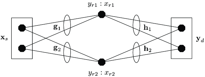
Refer to caption
Figure 1: System model
Refer to caption
Figure 2: Cut-set upper bounds

Refer to caption
(a) Optimal correlation versus φhsubscript𝜑\varphi_{h}
Refer to caption
(b) Optimal correlation versus SNRgsubscriptSNR𝑔\textsf{SNR}_{g}
Figure 3: Optimal correlation as a function of φhsubscript𝜑\varphi_{h} and SNRgsubscriptSNR𝑔\textsf{SNR}_{g}

Refer to caption
(a) φh=0subscript𝜑superscript0\varphi_{h}=0^{\circ}, |ρ|opt=1superscript𝜌𝑜𝑝𝑡1|\rho|^{opt}=1.
Refer to caption
(b) φh=25subscript𝜑superscript25\varphi_{h}=25^{\circ}, |ρ|opt=1superscript𝜌𝑜𝑝𝑡1|\rho|^{opt}=1.
Refer to caption
(c) φh=35subscript𝜑superscript35\varphi_{h}=35^{\circ}, |ρ|opt=0.5superscript𝜌𝑜𝑝𝑡0.5|\rho|^{opt}=0.5.
Refer to caption
(d) φh=90subscript𝜑superscript90\varphi_{h}=90^{\circ}, |ρ|opt=0superscript𝜌𝑜𝑝𝑡0|\rho|^{opt}=0.
Figure 4: SIMO MAC achievable regions with Pr1=Pr2=5subscript𝑃𝑟1subscript𝑃𝑟25P_{r1}=P_{r2}=5 and 𝐡𝟏=𝐡𝟐=1normsubscript𝐡1normsubscript𝐡21||\mathbf{h_{1}}||=||\mathbf{h_{2}}||=1

Refer to caption
(a) φh=0subscript𝜑superscript0\varphi_{h}=0^{\circ}, |ρ|opt=1superscript𝜌𝑜𝑝𝑡1|\rho|^{opt}=1.
Refer to caption
(b) φh=25subscript𝜑superscript25\varphi_{h}=25^{\circ}, |ρ|opt=1superscript𝜌𝑜𝑝𝑡1|\rho|^{opt}=1.
Refer to caption
(c) φh=35subscript𝜑superscript35\varphi_{h}=35^{\circ}, |ρ|opt=0.5superscript𝜌𝑜𝑝𝑡0.5|\rho|^{opt}=0.5.
Refer to caption
(d) φh=90subscript𝜑superscript90\varphi_{h}=90^{\circ}, |ρ|opt=0superscript𝜌𝑜𝑝𝑡0|\rho|^{opt}=0.
Figure 5: Sum-rate versus |ρ|𝜌|\rho| with Pr1=Pr2=5subscript𝑃𝑟1subscript𝑃𝑟25P_{r1}=P_{r2}=5 and 𝐡𝟏=𝐡𝟐=1normsubscript𝐡1normsubscript𝐡21||\mathbf{h_{1}}||=||\mathbf{h_{2}}||=1

Refer to caption
(a) Parallel channel vectors: φg=0subscript𝜑𝑔superscript0\varphi_{g}=0^{\circ}
Refer to caption
(b) Orthogonal channel vectors: φg=90subscript𝜑𝑔superscript90\varphi_{g}=90^{\circ}
Figure 6: MISO BC achievable regions with Ps=10subscript𝑃𝑠10P_{s}=10 and 𝐠1=𝐠2=1normsubscript𝐠1normsubscript𝐠21||\mathbf{g}_{1}||=||\mathbf{g}_{2}||=1

Refer to caption
(a) Three-dimensional region
Refer to caption
(b) Cross section along the surface R1=R2subscript𝑅1subscript𝑅2R_{1}=R_{2}
Figure 7: DF achievable region: P𝐬=10subscript𝑃𝐬10P_{\mathbf{s}}=10, Pr1=Pr2=4.17subscript𝑃𝑟1subscript𝑃𝑟24.17P_{r1}=P_{r2}=4.17, φg=φh=46.3942subscript𝜑𝑔subscript𝜑superscript46.3942\varphi_{g}=\varphi_{h}=46.3942^{\circ}, |ρ|opt=0.31superscript𝜌𝑜𝑝𝑡0.31\left|\rho\right|^{opt}=0.31 and Rcth=0.79superscriptsubscript𝑅𝑐𝑡0.79R_{c}^{th}=0.79.

Refer to caption
(a) Multiple DF optimal points.
Refer to caption
(b) Single DF optimal point.
Refer to caption
(c) No DF optimal point.
Refer to caption
(d) No DF optimal point.
Figure 8: Symmetric channels.

Refer to caption
(a) 𝐠1=1normsubscript𝐠11\left\|{\bf g}_{1}\right\|=1, 𝐠2=0.16normsubscript𝐠20.16\left\|{\bf g}_{2}\right\|=0.16 and bpeak=1.67superscript𝑏𝑝𝑒𝑎𝑘1.67b^{peak}=1.67
Refer to caption
(b) 𝐠1=1normsubscript𝐠11\left\|{\bf g}_{1}\right\|=1, 𝐠2=0.09normsubscript𝐠20.09\left\|{\bf g}_{2}\right\|=0.09 and bpeak=1.85superscript𝑏𝑝𝑒𝑎𝑘1.85b^{peak}=1.85
Figure 9: R(apeak,b)𝑅superscript𝑎𝑝𝑒𝑎𝑘𝑏R(a^{peak},b) versus b𝑏b with Ps=10subscript𝑃𝑠10P_{s}=10, Pr1=Pr2=5subscript𝑃𝑟1subscript𝑃𝑟25P_{r1}=P_{r2}=5, 𝐡1=𝐡2=1normsubscript𝐡1normsubscript𝐡21\left\|{\bf h}_{1}\right\|=\left\|{\bf h}_{2}\right\|=1 and φg=φh=46.40subscript𝜑𝑔subscript𝜑superscript46.40\varphi_{g}=\varphi_{h}=46.40^{\circ}

Refer to caption
(a) φg=90subscript𝜑𝑔superscript90\varphi_{g}=90^{\circ} and φh=90subscript𝜑superscript90\varphi_{h}=90^{\circ}.
Refer to caption
(b) φg=90subscript𝜑𝑔superscript90\varphi_{g}=90^{\circ} and φh=0subscript𝜑superscript0\varphi_{h}=0^{\circ}.
Refer to caption
(c) φg=46.3972subscript𝜑𝑔superscript46.3972\varphi_{g}=46.3972^{\circ} and φh=90subscript𝜑superscript90\varphi_{h}=90^{\circ}.
Refer to caption
(d) φg=46.3972subscript𝜑𝑔superscript46.3972\varphi_{g}=46.3972^{\circ} and φh=0subscript𝜑superscript0\varphi_{h}=0^{\circ}.
Refer to caption
(e) φg=0subscript𝜑𝑔superscript0\varphi_{g}=0^{\circ} and φh=90subscript𝜑superscript90\varphi_{h}=90^{\circ}.
Refer to caption
(f) φg=0subscript𝜑𝑔superscript0\varphi_{g}=0^{\circ} and φh=0subscript𝜑superscript0\varphi_{h}=0^{\circ}.
Figure 10: Upper bound and achievable rates versus relay power. Note that Ps=10subscript𝑃𝑠10P_{s}=10 (dB) and 𝐠1=𝐠2=𝐡1=𝐡2=1normsubscript𝐠1normsubscript𝐠2normsubscript𝐡1normsubscript𝐡21\left\|{\bf g}_{1}\right\|=\left\|{\bf g}_{2}\right\|=\left\|{\bf h}_{1}\right\|=\left\|{\bf h}_{2}\right\|=1.