A localization technique for ensemble Kalman filters

Abstract

Ensemble Kalman filter techniques are widely used to assimilate observations into dynamical models. The phase space dimension is typically much larger than the number of ensemble members which leads to inaccurate results in the computed covariance matrices. These inaccuracies can lead, among other things, to spurious long range correlations which can be eliminated by Schur-product-based localization techniques. In this paper, we propose a new technique for implementing such localization techniques within the class of ensemble transform/square root Kalman filters. Our approach relies on a continuous embedding of the Kalman filter update for the ensemble members, i.e., we state an ordinary differential equation (ODE) whose solutions, over a unit time interval, are equivalent to the Kalman filter update. The ODE formulation forms a gradient system with the observations as a cost functional. Besides localization, the new ODE ensemble formulation should also find useful applications in the context of nonlinear observation operators and observations arriving continuously in time.

Keywords. Data assimilation, ensemble Kalman filter, localization, continuous Kalman filter

1 Introduction

We consider ordinary differential equations

$$\dot{\bf x}=f({\bf x},t)$$ (1)

with state variable ${\bf x}\in\mathbb{R}^{n}$. Initial conditions at time $t_{0}$ are not precisely known and we assume instead that

$${\bf x}(t_{0})\sim{\rm N}({\bf x}_{0},{\bf B}),$$ (2)

where ${\rm N}({\bf x}_{0},{\bf B})$ denotes an $n$-dimensional Gaussian distribution with mean ${\bf x}_{0}\in\mathbb{R}^{n}$ and covariance matrix ${\bf B}\in\mathbb{R}^{n\times n}$. We also assume that we obtain measurements ${\bf y}(t_{i})\in\mathbb{R}^{k}$ at discrete times $t_{j}\geq t_{0}$, $j=0,1,\ldots,M$, subject to measurement errors, which are also Gaussian distributed with zero mean and covariance matrix ${\bf R}\in\mathbb{R}^{k\times k}$, i.e.,

$${\bf y}(t_{j})-{\bf H}{\bf x}(t_{j})\sim{\rm N}({\bf 0},{\bf R}).$$ (3)

Here ${\bf H}\in\mathbb{R}^{k\times n}$ is the (linear) measurement operator.

Data assimilation is the task to combine the model (1) (here assumed to be perfect), the knowledge about the initial conditions (2) and available measurements (3) in a prediction of the probability distribution of the solution at any time $t>t_{0}$. We refer to Lewis et al. (2006) for a detailed introduction and available approaches to data assimilation. In this paper, we focus on the ensemble Kalman filter (EnKF) method, originally proposed by Evensen (see Evensen (2006) for a recent account) and, in particular, on ensemble transform (Bishop et al., 2001), ensemble adjustment (Anderson, 2001), and ensemble square root filters (Tippett et al., 2003) and their sequential implementation (Whitaker and Hamill, 2002; Anderson, 2003).

The EnKF relies on the simultaneous propagation of $m$ independent solutions ${\bf x}_{i}(t)$, $i=1,\ldots,m$, from which we can extract an empirical mean

$$\overline{\bf x}(t)=\frac{1}{m}\sum_{i=1}^{m}{\bf x}_{i}(t)$$ (4)

and an empirical covariance matrix

$${\bf P}(t)=\frac{1}{m-1}\sum_{i=1}^{m}\left({\bf x}_{i}(t)-\overline{\bf x}(t)\right)\left({\bf x}_{i}(t)-\overline{\bf x}(t)\right)^{T}.$$ (5)

In typical applications from meteorology, the ensemble size $m$ is much smaller than the dimension $n$ of the model phase space and, more importantly, also much smaller than the number of positive Lyapunov exponents. Hence ${\bf P}(t)$ is highly rank deficient which can lead to unreliable predictions. Ensemble localization has been introduced by Houtekamer and Mitchell (2001) and Hamill et al. (2001) to overcome this problem. However, only two techniques are currently available to implement Schur-product-based localization within the framework of ensemble transform/square root Kalman filters. The first option is provided by a sequential processing of observations (Whitaker and Hamill, 2002; Anderson, 2003), while the deterministic ensemble Kalman filter (DEnKF) of Sakov and Oke (2008a) is a second, more recent, option. The DEnKF results in an approximate implementation of ensemble transform/square root Kalman filters. We also mention box/local analysis methods (Evensen, 2003; Ott et al., 2004; Hunt et al., 2007), which assimilate data locally in physical space and which therefore possess a “built in” localization.

In this paper, we demonstrate that techniques proposed by Bergemann et al. (2009) for the filter analysis step can be further generalized to an ordinary differential equation (ODE) formulation in terms of the ensemble members ${\bf x}_{i}$, $i=1,\ldots,m$. This formulation is subsequently used to derive an easy to implement localized ensemble Kalman filter, which can process observations simultaneously and can be extended to nonlinear observation operators.

2 Background material

We summarize a number of key results and techniques regarding ensemble Kalman filters. We refer to Evensen (2006) for an introduction and in-depth discussion of such filters.

2.1 Kalman analysis step

Let $n$ denote the dimension of the phase space of the problem. We consider an ensemble of $m$ members ${\bf x}_{i}(t)\in\mathbb{R}^{n}$ which we collect in a matrix ${\bf X}(t)\in\mathbb{R}^{n\times m}$. In terms of ${\bf X}$, the ensemble mean is given by

$$\overline{\bf x}(t)=\frac{1}{m}{\bf X}(t){\bf e}\in\mathbb{R}^{n}$$ (6)

and we introduce the ensemble deviation matrix

$${\bf X}^{\prime}(t)={\bf X}(t)-\overline{\bf x}(t){\bf e}^{T}\in\mathbb{R}^{n\times m},$$ (7)

where ${\bf e}=(1,\ldots,1)^{T}\in\mathbb{R}^{m}$.

We now describe the basic Kalman analysis step. Let $\overline{\bf x}_{f}$ and ${\bf X}^{\prime}_{f}$ denote the forecast mean and deviation matrix, respectively. The ensemble mean is updated according to

$$\overline{\bf x}_{a}=\overline{\bf x}_{f}-{\bf K}\left({\bf H}\overline{\bf x}_{f}-{\bf y}\right),$$ (8)

where

$${\bf K}={\bf P}_{f}{\bf H}^{T}\left({\bf H}{\bf P}_{f}{\bf H}^{T}+{\bf R}\right)^{-1}$$ (9)

is the Kalman gain matrix with empirical covariance matrix

$${\bf P}_{f}=\frac{1}{m-1}{\bf X}^{\prime}({\bf X}^{\prime})^{T},$$ (10)

and ${\bf R}\in\mathbb{R}^{k\times k}$ is the measurement error covariance matrix.

While the update of the mean is common to most ensemble Kalman filters, the update of the ensemble deviation matrix ${\bf X}^{\prime}_{f}$ can be implemented in several ways. In this paper, we focus on ensemble update techniques that employ either a transformation of the form

$${\bf X}^{\prime}_{a}={\bf A}{\bf X}^{\prime}_{f}$$ (11)

with an appropriate matrix ${\bf A}\in\mathbb{R}^{n\times n}$ (Anderson, 2001) or a transformation

$${\bf X}^{\prime}_{a}={\bf X}^{\prime}_{f}{\bf T}$$ (12)

with an appropriate ${\bf T}\in\mathbb{R}^{m\times m}$ (Bishop et al., 2001; Whitaker and Hamill, 2002; Tippett et al., 2003; Evensen, 2004). The matrices ${\bf A}$ and ${\bf T}$ are chosen such that the resulting ensemble deviation matrix ${\bf X}^{\prime}_{a}$ satisfies

$${\bf P}_{a}=\frac{1}{m-1}{\bf X}^{\prime}_{a}({\bf X}^{\prime}_{a})^{T}=\left({\bf I}-{\bf K}{\bf H}\right){\bf P}_{f}.$$ (13)

It has been shown by Tippett et al. (2003) that both formulations (11) and (12) can be made equivalent not only in terms of (13) but also in terms of the resulting ensemble deviation matrix ${\bf X}_{a}^{\prime}$. Since $n\gg m$ in most applications, formulation (12) is generally preferred except when working in a sequential framework (Anderson, 2003).

Note that the transformation matrix ${\bf T}$ should also satisfy ${\bf T}{\bf e}={\bf e}$ to guarantee ${\bf X}^{\prime}_{a}{\bf e}={\bf 0}$ (Wang et al., 2004; Livings et al., 2008; Sakov and Oke, 2008b). Otherwise, the update of the ensemble deviation matrix would affect the update of the ensemble mean.

Several methods have been proposed recently (including Sakov and Oke (2008a) and Bergemann et al. (2009)) that satisfy (13) only approximately. More specifically, Sakov and Oke (2008a) suggest to use (11) with

$${\bf A}={\bf I}-\frac{1}{2}{\bf K}{\bf H},$$ (14)

while Bergemann et al. (2009) use numerical approximations to the underlying ODE formulation

$$\frac{{\rm d}}{{\rm d}s}{\bf Y}=-\frac{1}{2m-2}{\bf Y}{\bf Y}^{T}{\bf H}^{T}{\bf R}^{-1}{\bf H}{\bf Y}$$ (15)

in a fictitious time $s\in[0,1]$ See, for example, Simon (2006) for a derivation of (15). The initial condition is ${\bf Y}(0)={\bf X}^{\prime}_{f}$ and the updated ensemble deviation matrix, which satisfies (13) exactly, is provided by the solution at time $s=1$, i.e.

$${\bf X}^{\prime}_{a}={\bf Y}(1).$$ (16)

A typical numerical implementation of (15) uses two or four time-steps with the forward Euler method (Bergemann et al., 2009). The resulting transformation of the forecast into the analyzed ensemble deviation matrix is of the form (11) with ${\bf A}$ defined through the time-stepping method.

Note that the Kalman gain matrix (9) is equivalent to

$${\bf K}={\bf P}_{a}{\bf H}^{T}{\bf R}^{-1},$$ (17)

which is advantageous in connection with (15) since only the inversion of the measurement error covariance matrix ${\bf R}\in\mathbb{R}^{k\times k}$ is now required to implement a complete Kalman analysis step. Algorithmically, one would first update the ensemble deviation matrix using (15), then form the analysed ensemble covariance matrix ${\bf P}_{a}={\bf X}_{a}^{\prime}[{\bf X}_{a}^{\prime}]^{T}/(m-1)$ as well as the Kalman gain matrix (17), and finally update the ensemble mean using (8).

All methods discussed so far have in common that the Kalman update increments for the ensemble mean and ensemble deviation matrix lie in a $m-1$ dimensional subspace, denoted by $\mathbb{S}_{f}\subset\mathbb{R}^{n}$. This space is defined by the range/image of the forecast ensemble deviation matrix ${\bf X}_{f}^{\prime}$. Bergemann et al. (2009) introduced a continuous matrix factorization algorithm for the ensemble ${\bf X}(t)$, which automatically produces orthogonal vectors that span $\mathbb{S}_{f}$.

It is common practice to apply variance inflation (Anderson and Anderson, 1999) to ${\bf X}^{\prime}(t_{j})$ before the forecasted ensemble is updated under the Kalman filter analysis step, i.e., the Kalman analysis step uses

$${\bf X}_{f}:=\overline{\bf x}(t_{j}){\bf e}^{T}+\delta\,{\bf X}^{\prime}(t_{j}),$$ (18)

where $\delta\geq 1$ is an inflation factor, instead of ${\bf X}_{f}={\bf X}(t_{j})$.

2.2 Localization

The idea of localization, as proposed by Houtekamer and Mitchell (2001), is to replace the matrices ${\bf H}{\bf P}_{f}$ and ${\bf H}{\bf P}_{f}{\bf H}^{T}$ in the Kalman gain matrix (9) by

$$\widetilde{{\bf H}{\bf P}_{f}}={\bf C}_{{\rm loc},1}\circ\left({\bf H}{\bf P}_{f}\right),\quad\widetilde{{\bf H}{\bf P}_{f}{\bf H}^{T}}={\bf C}_{{\rm loc},2}\circ\left({\bf H}{\bf P}_{f}{\bf H}^{T}\right),$$ (19)

respectively, where ${\bf C}_{{\rm loc},1}\in\mathbb{R}^{n\times k}$ and ${\bf C}_{{\rm loc},2}\in\mathbb{R}^{k\times k}$ are appropriate localization matrices based on filter functions suggested by (Gaspari and Cohn, 1999) and ${\bf C}\circ{\bf Y}$ denotes the Schur product of two matrices ${\bf C}$ and ${\bf Y}$ of identical dimension, i.e.,

$$\left({\bf C}\circ{\bf Y}\right)_{i,j}=({\bf C})_{i,j}\,({\bf Y})_{i,j}$$ (20)

for all indices $i,j$. We denote the resulting modified Kalman gain matrix by ${\bf K}_{\rm loc,f}$, i.e.,

$${\bf K}_{\rm loc,f}=(\widetilde{{\bf H}{\bf P}_{f}})^{T}\left(\widetilde{{\bf H}{\bf P}_{f}{\bf H}^{T}}+{\bf R}\right)^{-1}.$$ (21)

Localization was also proposed by Hamill et al. (2001) with the only difference that localization is not applied to ${\bf H}{\bf P}_{f}{\bf H}^{T}$.

Alternatively, one can localize the Kalman gain matrix formulation (17) and use

$${\bf K}_{\rm loc,a}=(\widetilde{{\bf H}{\bf P}_{a}})^{T}{\bf R}^{-1}$$ (22)

instead of (9) in an ensemble Kalman filter. Note that (21) and (22) are not equivalent in general and that formulation (22) is easier to implement.

Based on these modified Kalman gain matrices, a Schur-product-based localization is easy to apply to the update (8) of the ensemble mean and to ensemble deviation updates that use perturbed observations (Burgers et al., 1998), which is essentially the localization approach of Houtekamer and Mitchell (2001) and Hamill et al. (2001). However, the popular class of ensemble transform/square root filters, based on (12), has not yet been amenable to Schur-product-based localizations except when observations are treated sequentially, i.e., when $k=1$ in each transformation step (Whitaker and Hamill, 2002).

It is feasible that localizations can be implemented for ensemble deviation updates of the form (11) through an appropriate modification of the ensemble adjustment technique of Anderson (2001). However, such a modification would lead to a computationally expensive implementation of Schur-product-based localizations. The recently proposed DEnKF filter of Sakov and Oke (2008a), on the other hand, leads to a computationally feasible implementation with the localization directly applied to (14), i.e., one uses

$${\bf A}={\bf I}-\frac{1}{2}{\bf K}_{\rm loc,f}{\bf H}$$ (23)

in (11).

We note that localization implies in general that the update increments for the ensemble mean and the ensemble deviation matrix no longer lie in the subspace $\mathbb{S}_{f}$ defined by the range/image of ${\bf X}_{f}^{\prime}$. While this is a desirable property on the one hand, it can lead to unbalanced fields in the analyzed ensemble ${\bf X}_{a}$ on the other hand. This has been investigated, for example, by Houtekamer and Mitchell (2005) and Kepert (2009).

We finally mention an alternative approach to localization. The box/local EnKF filters of Evensen (2003); Ott et al. (2004); Hunt et al. (2007) assimilate data locally in physical space and possess a “built in” localization based on the spatial structure of the underlying partial differential equation model.

3 Localization based on continuous ensemble updates

We now describe an alternative for introducing localization, which is based on a generalization of the ODE formulation (15) and which leads to an ODE formulation directly in the ensemble members ${\bf x}_{i}$.

We first note that the Kalman update (8) for the ensemble mean can also be formulated in terms of an ODE, i.e.,

$$\frac{\rm d}{{\rm d}s}\overline{\bf x}=-\frac{1}{m-1}{\bf Y}{\bf Y}^{T}{\bf H}^{T}{\bf R}^{-1}\left({\bf H}\overline{\bf x}-{\bf y}\right)$$ (24)

with $\overline{\bf x}(0)=\overline{\bf x}_{f}$ and $\overline{\bf x}_{a}=\overline{\bf x}(1)$. See, for example, Simon (2006) for a derivation of (24).

To further reveal the underlying mathematical structure of (15) and (24), we introduce the cost functional

$$S({\bf x})=\frac{1}{2}\left({\bf H}{\bf x}-{\bf y}\right)^{T}{\bf R}^{-1}\left({\bf H}{\bf x}-{\bf y}\right)$$ (25)

for each set of observations. Next we combine (15) and (24) to give rise to the differential equations

$$\frac{\rm d}{{\rm d}s}{\bf x}_{i}=-\frac{1}{2}{\bf P}\left\{\nabla_{{\bf x}_{i}}S({\bf x}_{i})+\nabla_{\overline{\bf x}}S(\overline{\bf x})\right\}$$ (26)

in the ensemble members ${\bf x}_{i}$, $i=1,\ldots,m$. The equations are closed through the standard definition

$$\overline{\bf x}(s)=\frac{1}{m}\sum_{i=1}^{m}{\bf x}_{i}(s)$$ (27)

for the mean and covariance matrix

$${\bf P}(s)=\frac{1}{m-1}\sum_{i=1}^{m}\left({\bf x}_{i}(s)-\overline{\bf x}(s)\right)\left({\bf x}_{i}(s)-\overline{\bf x}(s)\right)^{T}.$$ (28)

Since the covariance matrix ${\bf P}$ is symmetric, a straightforward calculation reveals that

$$\frac{\rm d}{{\rm d}s}\left\{S(\overline{\bf x})+\frac{1}{m}\sum_{i=1}^{m}S({\bf x}_{i})\right\}\leq 0$$ (29)

along solutions of (26). More precisely, (26) is equivalent to the gradient system

$$\frac{\rm d}{{\rm d}s}{\bf x}_{i}=-{\bf P}\nabla_{{\bf x}_{i}}{\cal V}({\bf X}),$$ (30)

in the ensemble matrix ${\bf X}(s)$ with potential

$${\cal V}({\bf X})=\frac{m}{2}\left\{S(\overline{\bf x})+\frac{1}{m}\sum_{i=1}^{m}S({\bf x}_{i})\right\}.$$ (31)

The actual decay of the potential ${\cal V}$ along solutions of (30) depends crucially on the covariance matrix ${\bf P}$.

We note that Schur-product-based localizations can easily be applied to (26) to obtain, e.g.,

$$\frac{\rm d}{{\rm d}s}{\bf x}_{i}=-\frac{1}{2}\widetilde{\bf P}\left\{\nabla_{{\bf x}_{i}}S({\bf x}_{i})+\nabla_{\overline{\bf x}}S(\overline{\bf x})\right\},\qquad\widetilde{\bf P}={\bf C}_{\rm loc}\circ{\bf P},$$ (32)

or

$$\frac{\rm d}{{\rm d}s}{\bf x}_{i}=-\frac{1}{2}(\widetilde{\bf HP})^{T}{\bf R}^{-1}\left\{{\bf H}{\bf x}_{i}+{\bf H}\overline{\bf x}-2{\bf y}\right\},\qquad\widetilde{\bf HP}={\bf C}_{{\rm loc},1}\circ({\bf HP}),$$ (33)

in case of linear observation operators. These modified ensemble update formulations are easy to implement numerically. See Section 4 for details.

4 Numerical implementation aspects

The various ODE formulations for the ensemble members ${\bf x}_{i}$, $i=1,\ldots,m$, need to be solved over a unit time interval with initial conditions provided by the forecast values ${\bf x}_{i,f}$ of the ensemble members. We apply the forward Euler method with step-size $\Delta s=1/4$ (four time-steps) for our experiments. We found that $\Delta s=1$ (single time-step) and $\Delta s=1/3$ (three time-steps) lead to unstable simulations, while $\Delta s=1/2$ (two time-steps) leads to occasional instabilities for larger values of the ensemble inflation factor $\delta$ in (18). On the other hand, increasing the number of time-steps beyond four did not change the results significantly. We also expect that four time-steps will generally be sufficient in practical applications unless observations strongly contradict their forecast values and large gradient values are generated in (26). The same consideration can apply to simulations with large inflation factors $\delta$ in (18). As a safe guard, one can monitor the decay of the potential (31) along numerically generated solutions and adjust the step-size $\Delta s$ if necessary.

Note that the continuous formulations do not require matrix inversions/factorizations except for the computation of ${\bf R}^{-1}$. The computational cost of localization can be reduced even further by using the following approximation. The matrix $\widetilde{\bf HP}$ in (33) varies along solutions and an approximative formulation is obtained by replacing $\widetilde{{\bf H}{\bf P}}(s)$ by its value at $s=0$ for all $s>0$. This leads to a linear ODE in the ensemble members ${\bf x}_{i}$ with constant coefficient matrix, i.e.,

$$\frac{{\rm d}}{{\rm d}s}{\bf x}_{i}=-\frac{1}{2}(\widetilde{{\bf H}{\bf P}}(0))^{T}{\bf R}^{-1}\left\{{\bf H}{\bf x}_{i}+{\bf H}\overline{\bf x}-2{\bf y}\right\}.$$ (34)

Note that $\widetilde{\bf HP}$ and $\widetilde{{\bf HPH}^{T}}$ are sparse matrices for compactly supported filter functions (Gaspari and Cohn, 1999). Numerical implementations of (34) should first update the increments ${\bf z}_{i}={\bf H}{\bf x}_{i}-{\bf y}$ with Euler’s method, i.e.,

$${\bf z}_{i}^{l+1}={\bf z}_{i}^{l}-\frac{\Delta s}{2}\widetilde{{\bf HPH}^{T}}(0){\bf R}^{-1}\left\{{\bf z}_{i}^{l}+\frac{1}{m}\sum_{j=1}^{m}{\bf z}_{j}^{l}\right\},\qquad l=0,\ldots,L,$$ (35)

$L=1/\Delta s$ the number of integration steps, and then use the accumulated increments

$${\bf z}_{i}=\sum_{l=0}^{L-1}{\bf z}_{i}^{l}$$ (36)

to compute the final update of the ensemble members ${\bf x}_{i}$, $i=1,\ldots,m$. Overall matrix-vector-products will induce a computational complexity of ${\cal O}(k\,m)$ in the ensemble size $m$ and the number of observations $k$ independent of the system size $n$. The same order of complexity applies to the serial algorithm of Hamill et al. (2001) with the important difference that (34) can be implemented as a simultaneous update over all observations.

Bergemann et al. (2009) proposed a re-orthogonalization technique for the ensemble deviation matrix ${\bf X}^{\prime}$. It should be noted that the re-orthogonalization is not uniquely defined. We implemented several variants of re-orthogonalization in combination with localization but did not find any significant improvements in the results.

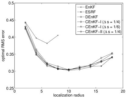
Figure 1: The best RMS error for the Lorenz-96 model with an ensemble size of $m=10$ and $k=20$ observations taken in intervals of $\Delta t_{\rm obs}=0.05$ over a total of 5000 assimilation cycles.

5 Numerical experiments

We now report results from two test problems and implementations of (33) and (34) with localization. The results are compared to those from standard ensemble Kalman filter techniques.

5.1 Lorenz-96 model

The standard implementation of the Lorenz-96 model (Lorenz, 1996; Lorenz and Emanuel, 1998) has state vector ${\bf x}=(x_{1},\ldots,x_{n})^{T}\in\mathbb{R}^{n}$, $n=40$, and its time evolution is given by the differential equations

$$\dot{x}_{j}=(x_{j+1}-x_{j-2})x_{j-1}-x_{j}+8$$ (37)

for $j=1,\ldots,n$. To close the equations, we define $x_{-1}=x_{39}$, $x_{0}=x_{40}$, and $x_{41}=x_{1}$.

The attractor of this standard implementation has a fractal dimension of about 27 and 13 positive Lyapunov exponents. Localization will be necessary for ensembles with $m\leq 13$ ensemble members. We use an ensemble size of $m=10$ in our experiments. We observe every second grid point, i.e., $k=20$, and the measurement error covariance is ${\bf R}={\bf I}_{20}$. Measurement are taken in time intervals of $\Delta t_{\rm obs}=0.05$. After a short spin-up period, a total of $J=5000$ analysis steps are performed in each experiment. The ”true” trajectory ${\bf x}_{\rm truth}(t_{n})$ is generated by integrating the Lorenz-96 model with the implicit midpoint rule and step-size $\Delta t=0.005$, i.e., we assume that there is no model error. The observations are obtained according to

$${\bf y}(t_{\rm obs})={\bf H}{\bf x}_{\rm truth}(t_{\rm obs})+{\bf r}(t_{\rm obs}),$$ (38)

where ${\bf r}(t_{\rm obs})$ are i.i.d. Gaussian random numbers with mean zero and covariance matrix ${\bf R}$.

We implement localization combined with standard ensemble inflation for the following five different ensemble Kalman filters: (i) EnKF with perturbed observations (Burgers et al., 1998; Houtekamer and Mitchell, 2005), (ii) ensemble square root filter (ESRF) with sequential treatment of observations (Whitaker and Hamill, 2002), (iii) DEnKF (Sakov and Oke, 2008a), (iv) formulation (33), denoted CEnKF-I, (v) formulation (34), denoted CEnKF-II. We implement CEnKF-I with $\Delta s=1/4$ and $\Delta s=1/6$, respectively, to demonstrate the impact of the discretization parameter on the results.

For simplicity, localization is performed by multiplying each element of the matrices ${\bf H}{\bf P}$ and ${\bf H}{\bf P}{\bf H}^{T}$, respectively, by a distance dependent factor $\rho_{i,i^{\prime}}$. This factor is defined by the compactly supported localization function (4.10) from Gaspari and Cohn (1999), distance $r_{i,i^{\prime}}=\min\{|i-i^{\prime}|,n-|i-i^{\prime}|\}$, where $i$ and $i^{\prime}$ denote the indices of the associated observation/grid points $x_{i}$ and $x_{i^{\prime}}$, respectively, and a fixed localization radius $r_{0}$. The localization radius is varied between $r_{0}=2$ and $r_{0}=30$. The inflation factor $\delta$ in (18) is taken from the range $[\sqrt{1.02},\sqrt{1.16}]$.

In Figure 1, we display the RMS error

$${\rm rmse}=\sqrt{\frac{1}{n\,J}\sum_{j=1}^{J}\|\overline{\bf x}(j\cdot\Delta t_{\rm obs})-{\bf x}_{\rm truth}(j\cdot\Delta t_{\rm obs})\|^{2}}$$ (39)

for an optimally chosen inflation factor $\delta$ as a function of the localization radius $r_{0}$. Results are displayed for those localization radii $r_{0}$ only, which lead to at least one simulation with a RMS error of less than one.

We conclude that EnKF yields the lowest filter skills while all other methods show an almost identical performance.

$\delta\backslash r_{0}$	5	10	15	20	25	30	35
1.02	0.59	0.62	0.72	0.96	1.41	Inf	Inf
1.06	0.80	0.67	0.62	0.65	0.79	0.99	1.66
1.10	1.09	0.85	0.72	0.69	0.75	1.04	1.13
1.14	1.38	1.01	0.84	0.77	0.78	0.88	1.40
1.18	Inf	1.18	0.96	0.84	0.82	0.86	1.35

Table 1: Mean RMS error for localized CEnKF-I over 4000 time steps as a functions of the localization radius $r_{0}$ and the inflation factor $\delta$. For clarity, the value Inf is assigned if the RMS error exceeds the value 2.0 (no filter skill).

$\delta\backslash r_{0}$	5	10	15	20	25	30	35
1.02	0.60	0.65	0.77	1.01	1.31	1.80	Inf
1.06	0.80	0.66	0.63	0.68	0.86	1.13	1.51
1.10	1.11	0.84	0.72	0.69	0.74	0.93	1.29
1.14	1.42	1.04	0.83	0.76	0.78	0.86	1.14
1.18	Inf	1.21	0.96	0.85	0.82	0.86	1.16

Table 2: Mean RMS error for localized CEnKF-II over 4000 time steps as a functions of the localization radius $r_{0}$ and the inflation factor $\delta$.

$\delta\backslash r_{0}$	5	10	15	20	25	30	35
1.02	0.59	0.62	0.75	0.94	1.06	Inf	Inf
1.06	0.82	0.69	0.64	0.68	0.73	0.98	Inf
1.10	1.16	0.89	0.75	0.70	0.72	0.85	1.22
1.14	1.50	1.11	0.89	0.80	0.77	0.85	0.99
1.18	Inf	1.33	1.05	0.91	0.87	0.87	1.01

Table 3: Mean RMS error for localized DEnKF over 4000 time steps as a functions of the localization radius $r_{0}$ and the inflation factor $\delta$.

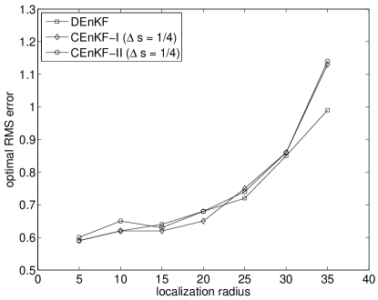
Figure 2: The best RMS error for the QG-model of Sakov and Oke (2008a) with an ensemble size of $m=25$ and $k=300$ observations taken in intervals of $\Delta t_{\rm obs}=4.0$ over a total of 1000 assimilation cycles.

5.2 A quasi-geostrophic (QG) model

We use the QG model of Sakov and Oke (2008a). The QG model is a numerical approximation of the following 1.5-layer reduced gravity quasi-geostrophic model with double-gyre wind forcing and biharmonic friction:

$$q_{t}=-\psi_{x}-\varepsilon J(\psi,q)-A\Delta^{3}\psi+2\pi\sin(2\pi y),$$ (40)

where $q=\Delta\psi-F\psi$, $J(\psi,q)=\psi_{x}q_{y}-\psi_{y}q_{x}$, $\Delta=\partial^{2}/\partial x^{2}+\partial^{2}/\partial y^{2}$. The coefficients are given by $F=1600$, $\varepsilon=$ 10^-5, $A=2\times$10^-12. The model domain is $(x,y)\in[0,1]\times[0,1]$ with zero Dirichlet boundary conditions. The model is discretized over this domain using a $129\times 129$ grid. For more details see Sakov and Oke (2008a).

We implement the deterministic ensemble Kalman filter (DEnKF) and our ensemble Kalman filters based on (33). All experiments use $m=25$ ensemble members. The dimension of the phase space is $n=16129$. The dimension of the attractor and the number of positive Lyapunov exponents are currently not known.

In line with Sakov and Oke (2008a), localization is performed by multiplying each element of the matrices ${\bf H}{\bf P}$ and ${\bf H}{\bf P}{\bf H}^{T}$, respectively, by a factor $\rho_{ij,i^{\prime}j^{\prime}}=\exp(-0.5r_{ij,i^{\prime}j^{\prime}}^{2}/r_{0}^{2})$. Here we use the distance $r_{ij,i^{\prime}j^{\prime}}=\sqrt{|i-i^{\prime}|^{2}+|j-j^{\prime}|^{2}}$, where $(i,j)$ and $(i^{\prime},j^{\prime})$ denote the indices of the associated observation/grid points $x_{ij}$ and $x_{i^{\prime}j^{\prime}}$, respectively, and $r_{0}$ is a fixed localization radius.

We test the performance of the filters for different values of the ensemble inflation factor $\delta$ in (18) and the localization radius $r_{0}$. For each pair $(\delta,r_{0})$ of simulation parameters, we run a single simulation over 4000 time steps with step-size $\Delta t=1.25$ and perform a total of 1000 assimilation cycles using 300 observations of $\psi$ with observation variance of 4.0 as described in Sakov and Oke (2008a) (after a spin-up period of 200 time steps and 50 assimilation cycles). All simulations are started from the same initial ensemble and use identical sets of observations.

Since the DEnKF has been compared with EnKF and ESRF by Sakov and Oke (2008a) and showed the best performance of all tested methods for this test problem, we only perform a comparison between the new formulations CEnKF-I (based on (33) with $\Delta s=1/4$), CEnKF-II (based on (34) with $\Delta s=1/4$) and DEnKF. The mean RMS errors of all three methods can be found in Tables 2 to 3. In Figure 2, we display the RMS error for an optimally chosen inflation factor $\delta$ as a function of the localization radius $r_{0}$. Curves are based on the data presented in Tables 2 to 3. We conclude from Figure 2 that all three filters display a nearly identical performance for an optimal $(\delta,r_{0})$ parameter choice and that DEnKF shows a slightly better performance for the largest localization radius $r_{0}=35$. A similar observation was made by Sakov and Oke (2008a) with regard to a comparison between DEnKF and ESRF. The differt results for $r_{0}=35$ could be due to the built-in overestimation of the analyzed ensemble covariance matrix (Sakov and Oke, 2008a).

It should be noted that CEnKF-II is the least computational expensive of the three methods considered in this study.

6 Conclusions and further extensions

Schur-product-based localization of covariance matrices has become a popular and powerful tool to make ensemble Kalman filters perform well even under small ensemble sizes. In this note, we have proposed a new approach to implement Schur-product-based localization seamlessly within the framework of ensemble Kalman filters. Our approach is based on the formulation of the Kalman update step as differential equations in terms of its ensemble members. We have demonstrated for the Lorenz-96 model that the resulting methods outperform EnKF with perturbed observations and perform as well as standard implementations of ensemble Kalman filters such as ESRF with serial processing of observations and the recently proposed DEnKF. We also implemented a QG model and found that our methods perform nearly as well as DEnKF which is currently the best available method for this model problem. From a computational point of view, the formulation (34) is particularly appealing since it leads to very efficient implementations without the need of matrix inversions (except when the error covariance matrix ${\bf R}$ is not diagonal) and only a single evaluation of the ensemble generated covariance matrix $\widetilde{\bf HP}$.

We now outline an number of possible extensions of the formulation (30).

First we note that (26) can be used in connection with any cost functional $S({\bf x})$ and, hence, provides a straightforward generalization of EnKF to nonlinear observation operators ${\bf y}={\bf h}({\bf x})$, i.e.,

$$S({\bf x})=\frac{1}{2}\left({\bf h}({\bf x})-{\bf y}\right)^{T}{\bf R}^{-1}\left({\bf h}({\bf x})-{\bf y}\right).$$ (41)

Second, as for other localization techniques, the formulation (32) leads to updates in the ensemble deviations ${\bf X}_{a}^{\prime}$ which lie outside the space $\mathbb{S}_{f}$ in general and, hence, may introduce imbalance into the analyzed ensemble members ${\bf x}_{i}$. It seems feasible to restore balance within the proposed framework by introducing additional cost functions $S_{\rm pseudo}({\bf x})$ into the formulations (32) or (33), respectively. For example, we might require that the divergence of a velocity field ${\bf v}$ remains “small” by including a cost functional

$$S_{\rm pseudo}=\frac{1}{2r}\int_{\Omega}\left(\nabla\cdot{\bf v}\right)^{2}\,{\rm d}V,$$ (42)

where $r>0$ is an appropriate constant. Hence we would modify (26) to

$$\frac{\rm d}{{\rm d}s}{\bf x}_{i}=-\frac{1}{2}{\bf P}\left[\nabla_{{\bf x}_{i}}\left\{S({\bf x}_{i})+S_{\rm pseudo}({\bf x}_{i})\right\}+\nabla_{\overline{\bf x}}\left\{S(\overline{\bf x})+S_{\rm pseudo}(\overline{\bf x})\right\}\right].$$ (43)

Third, we have focused on deterministic ensemble Kalman filter formulations in this paper. However, EnKF with perturbed observations (Burgers et al., 1998) can also be put into the framework of continuous updates and leads naturally to the formulation

$$\frac{\rm d}{{\rm d}s}{\bf x}_{i}=-{\bf P}{\bf H}^{T}{\bf R}^{-1}\left\{{\bf H}{\bf x}_{i}-{\bf y}_{i}\right\},$$ (44)

where ${\bf y}_{i}$ are now stochastically perturbed observations (Burgers et al., 1998). Alternatively, we may consider the stochastic differential equation

$${\rm d}{\bf x}_{i}=-{\bf P}{\bf H}^{T}{\bf R}^{-1}\left\{{\bf H}{\bf x}_{i}{\rm d}s-{\bf y}{\rm d}s+{\bf R}^{1/2}{\rm d}{\bf w}_{i}\right\}$$ (45)

in the ensemble members, where ${\bf w}_{i}(s)\in\mathbb{R}^{k}$ denotes standard $k$-dimensional Brownian motion. See, for example, Gardiner (2004) for an introduction to stochastic differential equations.

Fourth, we have extensively discussed the continuous formulation of a single Kalman filter analysis step for a set of observations given at some time instance $t_{j}$. We now come back to the complete ensemble Kalman filter formulation for sequences of observations at time instances $t_{j}$, $j=1,\ldots,M$, and intermediate propagation of the ensemble under the dynamics (1). The continuous formulation of the ensemble Kalman filter step allows for the following concise formulation in terms of a differential equation

$$\dot{\bf x}_{i}=f({\bf x}_{i})-\sum_{j=1}^{M}\delta(t-t_{j})\,{\bf P}\nabla_{{\bf x}_{i}}{\cal V}_{j}({\bf X})$$ (46)

in each ensemble member, where $\delta(\cdot)$ denotes the standard Dirac delta function and ${\cal V}_{j}({\bf X})$ is the potential (31) with $S({\bf x})$ replaced by

$$S_{j}({\bf x})=\frac{1}{2}\left({\bf H}{\bf x}-{\bf y}(t_{j})\right)^{T}{\bf R}^{-1}\left({\bf H}{\bf x}-{\bf y}(t_{j})\right).$$ (47)

One may view (46) as the original ODE (1) driven by a sequence of impluse like contributions due to observations. Numerically, it makes sense to regularize these impulses and to replace (46) by

$$\dot{\bf x}_{i}=f({\bf x}_{i})-\sum_{j=1}^{M}\delta_{\varepsilon}(t-t_{j})\,{\bf P}\nabla_{{\bf x}_{i}}{\cal V}_{j}({\bf X}),$$ (48)

where

$$\delta_{\varepsilon}(s)=\frac{1}{\varepsilon}\psi(s/\varepsilon),$$

$\psi(s)$ is the standard hat function (or a mollifier in the sense of Friedrichs (1944)), and $\varepsilon>0$ is an appropriate parameter. Formulation (48) can be solved numerically by any standard ODE solver. There is no longer a strict separation between ensemble propagation and filtering. Of course, the ODE (48) becomes extremely stiff as $\varepsilon\to 0$. A sensible choice is $\varepsilon\sim\Delta t$, where $\Delta t$ is the natural step-size for the ODE (1). The mollified formulation (48) might be of particular interest in the context of the assimilation of non-synoptic measurements, e.g., measurements which are arriving semi-continuously in time (see Evensen (2006) for a discussion of alternative approaches).

References

- Anderson [2001] J.L. Anderson. An ensemble adjustment filter for data assimilation. Mon. Wea. Rev., 129:2884–2903, 2001.
- Anderson [2003] J.L. Anderson. A local least squares framework for ensemble filtering. Mon. Wea. Rev., 131:634–642, 2003.
- Anderson and Anderson [1999] J.L. Anderson and S.L. Anderson. A Monte Carlo implementation of the nonlinear filtering problem to produce ensemble assimilations and forecasts. Mon. Wea. Rev., 127:2741–2758, 1999.
- Bergemann et al. [2009] K. Bergemann, G. Gottwald, and S. Reich. Ensemble propagation and continuous matrix factorization algorithms. Q. J. R. Meteorological Soc., 135:1560–1572, 2009.
- Bishop et al. [2001] C.H. Bishop, B. Etherton, and S.J. Majumdar. Adaptive sampling with the ensemble transform Kalman filter. Part I: Theoretical aspects. Mon. Wea. Rev., 129:420–436, 2001.
- Burgers et al. [1998] G. Burgers, P.J. van Leeuwen, and G. Evensen. On the analysis scheme in the ensemble Kalman filter. Mon. Wea. Rev., 126:1719–1724, 1998.
- Evensen [2006] G. Evensen. Data assimilation. The ensemble Kalman filter. Springer-Verlag, New York, 2006.
- Evensen [2003] G. Evensen. The Ensemble Kalman Filter: Theoretical formulation and practical implementation. Ocean Dynamics, 53:343–367, 2003.
- Evensen [2004] G. Evensen. Sampling strategies and square root analysis schemes for the EnKF. Ocean Dyn., 54:539–560, 2004.
- Friedrichs [1944] K.O. Friedrichs. The identity of weak and strong extensions of differential operators. Trans. Am. Math. Soc., 55:132–151, 1944.
- Gardiner [2004] C.W. Gardiner. Handbook on stochastic methods. Springer-Verlag, 3rd edition, 2004.
- Gaspari and Cohn [1999] G. Gaspari and S.E. Cohn. Construction of correlation functions in two and three dimensions. Q. J. Royal Meteorological Soc., 125:723–757, 1999.
- Hamill et al. [2001] Th.M. Hamill, J.S. Whitaker, and Ch. Snyder. Distance-dependent filtering of background covariance estimates in an ensemble Kalman filter. Mon. Wea. Rev., 129:2776–2790, 2001.
- Houtekamer and Mitchell [2001] P.L. Houtekamer and H.L. Mitchell. A sequential ensemble Kalman filter for atmospheric data assimilation. Mon. Wea. Rev., 129:123–136, 2001.
- Houtekamer and Mitchell [2005] P.L. Houtekamer and H.L. Mitchell. Ensemble Kalman filtering. Q. J. Royal Meteorological Soc., 131:3269–3289, 2005.
- Hunt et al. [2007] B.R. Hunt, E.J. Kostelich, and I. Szunyogh. Efficient data assimilation for spatialtemporal chaos: A local ensemble transform Kalman filter. Physica D, 230:112–137, 2007.
- Kepert [2009] J.D. Kepert. Covariance localisation and balance in an ensemble Kalman Filter. Q. J. Royal Meteorological Soc., 135:1157–1176, 2009.
- Lewis et al. [2006] J.M Lewis, S. Lakshmivarahan, and S.K. Dhall. Dynamic data assimilation: A least squares approach. Cambridge University Press, Cambridge, 2006.
- Livings et al. [2008] D.M. Livings, S.L. Dance, and N.K. Nichols. Unbiased ensemble square root filters. Physica D, 237:1021–1028, 2008.
- Lorenz [1996] E.N. Lorenz. Predictibility: A problem partly solved. In Proc. Seminar on Predictibility, volume 1, pages 1–18, ECMWF, Reading, Berkshire, UK, 1996.
- Lorenz and Emanuel [1998] E.N. Lorenz and K.E. Emanuel. Optimal sites for suplementary weather observations: Simulations with a small model. J. Atmos. Sci., 55:399–414, 1998.
- Ott et al. [2004] E. Ott, B.R. Hunt, I. Szunyogh, A.V. Zimin, E.J. Kostelich, M. Corazza, E. Kalnay, D.J. Patil, and J A. Yorke. A local ensemble Kalman filter for atmospheric data assimilation. Tellus, A 56:415–428, 2004.
- Sakov and Oke [2008a] P. Sakov and P.R. Oke. A deterministic formulation of the ensemble Kalman filter: An alternative to ensemble square root filters. Tellus, 60A:361–371, 2008a.
- Sakov and Oke [2008b] P. Sakov and P.R. Oke. Implications of the form of the ensemble transformation in the ensemble square root filter. Mon. Wea. Rev., 136:1042–1053, 2008b.
- Simon [2006] D.J. Simon. Optimal state estimation. John Wiley & Sons, Inc., New York, 2006.
- Tippett et al. [2003] M.K. Tippett, J.L. Anderson, G.H. Bishop, T.M. Hamill, and J.S. Whitaker. Ensemble square root filters. Mon. Wea. Rev., 131:1485–1490, 2003.
- Wang et al. [2004] X. Wang, C.H. Bishop, and S.J. Julier. Which is better, an ensemble of positive-negative pairs or a centered spherical simplex ensemble? Mon. Wea. Rev., 132:1590–1505, 2004.
- Whitaker and Hamill [2002] J. Whitaker and T.M. Hamill. Ensemble data assimilation without perturbed observations. Mon. Wea. Rev., 130:1913–1924, 2002.