Matter-wave dark solitons: stochastic vs. analytical results

Abstract

The dynamics of dark matter-wave solitons in elongated atomic condensates are discussed at finite temperatures. Simulations with the stochastic Gross-Pitaevskii equation reveal a noticeable, experimentally observable spread in individual soliton trajectories, attributed to inherent fluctuations in both phase and density of the underlying medium. Averaging over a number of such trajectories (as done in experiments) washes out such background fluctuations, revealing a well-defined temperature-dependent temporal growth in the oscillation amplitude. The average soliton dynamics is well captured by the simpler dissipative Gross-Pitaevskii equation, both numerically and via an analytically-derived equation for the soliton center based on perturbation theory for dark solitons.

Introduction. Atomic Bose-Einstein condensates (BECs) constitute ideal systems for studying nonlinear macroscopic excitations in quantum systems BEC_Book . Excitations in the form of dark solitons and vortices are known to arise spontaneously upon crossing the phase transition Spontaneous_Soliton ; Spontaneous_Vortex , a feature also studied in high-energy Kinks and condensed-matter Condensed_Solitons systems, in dynamical processes Soliton_Dynamical and through controlled engineering DarkSoliton_Burger ; DarkSoliton_Denschlag ; DarkSoliton_Hamburg_Nature ; DarkSoliton_Hamburg_PRL ; DarkSoliton_Heidelberg_PRL ; Vortex_Matthews_Madison . In the latter category dark solitons are imprinted in a controlled manner after the gas has equilibrated DarkSoliton_Burger ; DarkSoliton_Denschlag ; DarkSoliton_Hamburg_Nature ; DarkSoliton_Hamburg_PRL ; DarkSoliton_Heidelberg_PRL . Although thermal effects revealed rapid soliton decay near the condensate edge DarkSoliton_Burger ; Soliton_ZNG , recent experiments at reduced temperatures ($T\ll 0.5T_{c}$) DarkSoliton_Hamburg_Nature ; DarkSoliton_Hamburg_PRL ; DarkSoliton_Heidelberg_PRL found the predicted Busch_Anglin oscillatory pattern for the averaged soliton trajectories.

To date, finite temperature dynamics of dark solitons have been investigated with phenomenological Phenomenological , quasiparticle scattering Shlyapnikov , and generalised mean field Soliton_ZNG models; see also Quantum_Soliton_1 ; Quantum_Soliton_2 for quantum effects in various background potentials. The former predict oscillations with increasing amplitude (‘anti-damping’ Busch_Anglin ), and appear to reproduce the average soliton trajectories to varying degrees of accuracy, however fail to account for the random nature of the experiments. In particular, experiments showed variations from shot to shot DarkSoliton_Hamburg_Nature ; DarkSoliton_Hamburg_PRL ; DarkSoliton_Heidelberg_PRL , with single experimental realisations revealing the existence of dark solitons for times much longer than those for which a reproducible (or average) pattern can be generated, an effect attributed to ‘preparation errors’ DarkSoliton_Hamburg_Nature .

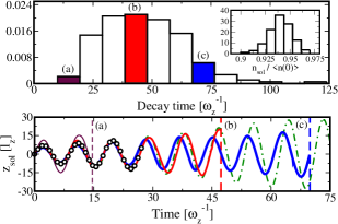
Figure 1: (Color online) Top: Normalised histograms of soliton decay times (main) and initial soliton depth, $n_{sol}$, scaled to the average peak density $\langle n(0)\rangle$ (inset) (based on 200 realisations). Bottom: Individual stochastic trajectories from marked histogram bins (for as long as they are numerically tractable), 10-realisation trajectory average (black circles) and DGPE trajectory (green, dash-dotted). (Parameters: $N\approx 20000$ ⁸⁷Rb atoms, $T=175$nK, $\omega_{z}=2\pi\times 10$Hz, $\omega_{\perp}=2\pi\times 2500$Hz, $|v|=0.25c$.)

In this Letter we show that a spread in the trajectories of dark solitons prepared in the same manner could also arise due to the critical dependence of individual solitons on local phase/density fluctuations. Modeling the soliton dynamics by the Stochastic Gross-Pitaevskii Equation (SGPE) SGPE_Stoof ; SGPE_Davis enables us to: (i) obtain an ab initio calculation of the spread of individual soliton trajectories (Fig. 1, top); (ii) demonstrate that although averaging over different trajectories generates a well-defined pattern, this is restricted to times much less than the longest observed trajectories (Fig. 1, bottom), consistent with experimental findings DarkSoliton_Hamburg_Nature ; DarkSoliton_Hamburg_PRL ; DarkSoliton_Heidelberg_PRL ; (iii) show that results based on stochastic trajectory averaging can be well captured by the dissipative GPE (DGPE) Phenomenological ; lp ; choi ; ueda , with an ab initio obtained damping coefficient; (iv) derive an analytical equation for the soliton center which captures such average dynamics very well at low temperatures.

Stochastic Dynamics: The SGPE SGPE_Stoof ; SGPE_Davis describes the condensate and lowest excitations in a unified manner, including both density and phase fluctuations, with irreversibility and damping arising from the coupling of such modes to a thermal particle reservoir. Assuming a ‘classical’ approximation for the mode occupations and a thermal cloud close to equilibrium, the SGPE reads SGPE_Stoof

$$i\hbar\partial_{t}\psi=(1-i\gamma)\left[\frac{\hbar^{2}}{2m}\partial_{z}^{2}+V(z)+g|\psi|^{2}-\mu\right]\psi+\eta\;,$$ (1)

where $g=2a\hbar\omega_{\perp}$ is the effective 1D coupling constant ($a$ is the scattering length, $\omega_{\perp}\gg\omega_{z}$ the transverse harmonic confinement), and $V(z)=(1/2)m\omega_{z}^{2}z^{2}$ the axial confining potential. $\gamma=i\beta\hbar\Sigma^{\rm K}(z,t)/4$ represents the ab initio determined dissipation arising due to the coupling to the thermal cloud ($\beta=1/k_{\rm B}T$). $\Sigma^{\rm K}(z,t)$ is the Keldysh self-energy due to incoherent collisions between condensate and non-condensate atoms and $\eta$ is a noise term with gaussian correlations $\langle\eta^{*}(z,t)\eta(z^{\prime},t^{\prime})\rangle=2\hbar k_{B}T\gamma(z,t)\delta(z-z^{\prime})\delta(t-t^{\prime})$ (see also SGPE_Stoof ; SGPE_Applications for further details and applications to condensate properties).

Soliton experiments are modelled by first letting the system equilibrate at a given temperature and then introducing a dark soliton of specified velocity $v$ in the trap center by multiplying $\psi$ by $\psi_{\rm sol}=\zeta{\rm tanh}(\zeta z/\xi)+i(v/c)$, where $\zeta=\sqrt{1-(v/c)^{2}}$ ($\xi$: healing length, $c$: speed of sound). Although the soliton generation is identical in all realisations (specified by $v/c$), fluctuations inherent in the atomic medium lead to a large variation in the imprinted soliton: The soliton speed $v/c=\sqrt{1-n_{d}/n}={\rm cos}(S/2)$ is closely related to the depth of the density minimum ($n_{d}$) and the phase slip $S$ across it. As a result, fluctuations in the background density upon generation should modify its depth, whereas the speed should also be affected by fluctuations in the condensate phase.

The combination of these two factors leads to a slightly asymmetric spread in the initial soliton depth (Fig. 1, top inset), also interpreted as a stochastic change in the initial soliton speed ($\approx 30\%$ for Fig. 1). Moreover, the ensuing trajectory is further modified by the local phase/density fluctuations during the SGPE evolution.

Soliton experiments are typically conducted in highly elongated geometries, in order to avoid dynamical instabilities Dynamical_Instabilities . Phase fluctuations in such geometries set in at a characteristic temperature $T_{\phi}$ Low_D_Geometries , which can be much lower than the corresponding ‘critical’ temperature $T_{c}$ K_vD_Tc1d . Although recent experiments DarkSoliton_Hamburg_Nature ; DarkSoliton_Hamburg_PRL ; DarkSoliton_Heidelberg_PRL were conducted in the regime $T\ll T_{\phi},T_{c}$, where both density and phase fluctuations are largely suppressed, soliton oscillations can still be observed in the presence of phase fluctuations ($T\gg T_{\phi}$), provided $T\ll T_{c}$. To amplify the differences between individual trajectories, we thus choose realistic experimental parameters ($N\approx 20000$ ⁸⁷Rb atoms, $\omega_{z}=2\pi\times 10$Hz, $\omega_{\perp}=250\omega_{z}$) corresponding to this intermediate regime $T_{\phi}\ll T\ll T_{c}$. This gives a phase coherence length $L_{\phi}\approx(0.1-0.25)R$ ($R$: Thomas-Fermi radius), with solitons allowed by $L_{\phi}\gg\xi$. We focus on a relatively deep soliton which is more prone to this effect; we also anticipate phase imprinting to further enhance differences in trajectories due to the effect of fluctuations during the initial state preparation Quantum_Soliton_2 .

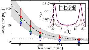
Figure 2: (Color online) Mean soliton decay times as a function of temperature obtained from the SGPE (red circles), or single DGPE realisations with ab initio determined $\gamma(z)$ (green diamonds), or averaged $\bar{\gamma}$ over $[-R/2,R/2]$ (blue squares). Grey band indicates SGPE values within one standard deviation of the mean decay time (for 200 runs); DGPE data shows time for soliton to decay to a depth comparable to the average background density fluctuations, with error bars corresponding to depths within the standard deviation of the fluctuations. Dotted horizontal line indicates time for one oscillation. Inset: $\gamma(z)$ (solid) for $T=150$ nK (bottom) and $300$ nK with $\bar{\gamma}$ (horizontal) for T=300nK; vertical lines show $R=28l_{z}$ (parameters as in Fig. 1; characteristic temperatures in 1D: $T_{\phi}=N(\hbar\omega_{z})^{2}/k_{B}\mu\approx 25$ nK Low_D_Geometries , $T_{c}=N\hbar\omega_{z}/k_{B}{\rm ln}(2N)\approx 900$ nK K_vD_Tc1d ).

Typical trajectories are shown in Fig. 1 (bottom) up to the point where the soliton can be numerically identified over the fluctuating background, which sets a decay time for each realisation. We find an asymmetric distribution of decay times, with some very long-lived trajectories. The spread in the decay times can be best visualised via characteristic trajectories from different histogram bins (labelled (a)-(c)). Despite their apparent differences, averaging over a sufficient number of trajectories (typically $\geq 10$) washes out such sensitivity, generating an antidamped oscillatory pattern, with a temperature-dependent shift in both amplitude and phase (black circles). The average trajectory is only defined up to the earliest decay time within the set of trajectories considered (here $27\omega_{z}^{-1}$), in analogy to the experimentally reproducible soliton dynamics being restricted to much shorter times than those of individual long-lived trajectories DarkSoliton_Hamburg_Nature ; DarkSoliton_Hamburg_PRL ; DarkSoliton_Heidelberg_PRL . The average trajectory is practically indistinguishable from an individual trajectory taken from the mean decay time bin (solid red), enabling us to infer the subsequent average soliton evolution from a single trajectory with a decay time close to the mean.

Fig. 2 shows the dependence of the soliton decay time on temperature (red circles) in the intermediate temperature range of noticeable anti-damping: At higher $T$ the soliton is lost to the fluctuating background, prior to executing one full oscillation, thus leading to a decrease in the width of the decay time histogram, and to smaller error bars in the mean decay time; although our model predicts very little damping for $T\leq 100$ nK $\approx 10\%T_{\rm c}$, consistent with recent pure condensate experiments DarkSoliton_Heidelberg_PRL , our results may overestimate the actual lifetimes, due to the neglected role of collisions in the thermal cloud Soliton_ZNG .

The distribution of imprinted solitons and decay times is the main numerical result of this paper. Nonetheless, dynamics consistent with the average stochastic results can also be obtained by a simpler model discussed below.

The DGPE and its comparison with the SGPE. A dissipative mean-field equation similar in form to Eq. (1), but without a noise term, was first introduced in a phenomenological manner by Pitaevskii lp ; in the BEC context this was applied to damping of excitations choi , vortex lattice growth ueda ; gard and dark soliton decay Phenomenological . A numerical advantage of the DGPE (which also restricts its predictive ability) is that only a single realisation is required under the assumption that trajectory-averaged properties should only depend on the dissipation; this is shown in Fig. 2 (inset): the self-consistent inclusion Footnote_Gamma of the mean field potential $2g\langle|\psi|^{2}\rangle$ in the expression for $\gamma$ generates a relatively flat profile around the trap center, with peaks at the condensate edges where the thermal cloud density is greatest. Since in the relevant dark soliton studies, the soliton spends most of its time well within the condensate, we can extract an averaged dissipation $\bar{\gamma}$, over a spatially-restricted region, e.g. $\bar{\gamma}=\int\gamma(z)dz/R$, within $[-R/2,\,\,R/2]$. A simple analytical formula in the literature predicts $\gamma(0)=\alpha(ma^{2}k_{B}T/\pi\hbar^{2})$, with $\alpha\approx 3$ gard . We find the spatially averaged rate $\bar{\gamma}$ reveals a more pronounced scaling with temperature, though a reasonable first estimate can be obtained in the examined temperature range using this formula with $1/2<\alpha<4$.

At low temperatures, the DGPE soliton oscillations are practically indistinguishable from the SGPE ones (Fig. 1, bottom). A systematic comparison can be done by quantitatively comparing soliton decay times (Fig. 2): in the DGPE, these are identified by the time taken for the soliton to decay to a depth comparable to the background density fluctuations (as predicted here by a single SGPE run, or, in general, measured experimentally). We find very good agreement for both $\gamma(z)$ and $\bar{\gamma}$, within the error bars (grey bands), with a smaller relative error at lower temperatures. Since the DGPE reproduces the averaged results well in this regime (see also Fig. 3 below), we now provide an analytical solution for the soliton evolution.

Analytical Results. Upon dropping the position dependence of $\gamma(z)$ and further introducing the transformation $t\rightarrow(1+\gamma^{2})t$, the 1D DGPE takes the form:

$$(i-\gamma)\partial_{t}\psi=\left[\frac{1}{2}\partial_{z}^{2}+V(z)+|\psi|^{2}-\mu\right]\psi,$$ (2)

where the density $|\psi|^{2}$, length, time and energy are respectively measured in units of $2a$, $a_{\perp}=\sqrt{\hbar/m\omega_{\perp}}$, $\omega_{\perp}^{-1}$ and $\hbar\omega_{\perp}$, and $V(z)=(1/2)\Omega^{2}z^{2}$, with $\Omega=\omega_{z}/\omega_{\perp}\ll 1$. We seek a solution of Eq. (2) in the form $\psi(z,t)=\psi_{b}(z,t){\rm e}^{-i\theta(t)}\upsilon(z,t)$, where $\psi_{b}(z,t)$ and $\theta(t)$ denote the background amplitude and phase respectively, while the dark soliton $\upsilon(z,t)$ is governed by

$$i\partial_{t}\upsilon+\frac{1}{2}\partial_{z}^{2}\upsilon-\psi_{b}^{2}(|\upsilon|^{2}-1)\upsilon=-\frac{\partial_{z}\psi_{b}}{\psi_{b}}\partial_{z}\upsilon+\gamma\partial_{t}\upsilon.$$ (3)

We assume that the condensate dynamics involves a fast scale of relaxation of the background to the ground state (justified a posteriori) and that the dark soliton subsequently evolves on top of the relaxed ground state. In the Thomas-Fermi limit, $\psi_{b}^{2}\approx\mu-V(z)$, and rescaling $t\rightarrow\mu t$, $z\rightarrow\sqrt{\mu}z$, we obtain from Eq. (3) a perturbed nonlinear Schrödinger (NLS) equation:

$$i\partial_{t}\upsilon+\frac{1}{2}\partial_{z}^{2}\upsilon-(|\upsilon|^{2}-1)\upsilon=P(\upsilon),$$ (4)

where $P(\upsilon)$ stands for the total perturbation, namely,

$$P(\upsilon)=\frac{1}{2\mu^{2}}\left[2\left(1-|\upsilon|^{2}\right)V\upsilon+\frac{dV}{dz}\partial_{z}\upsilon+2\gamma\mu\partial_{t}\upsilon\right],$$ (5)

and all terms in $P$ are assumed to be of the same order ($\gamma\sim\Omega$). We now apply the perturbation theory for matter-wave dark solitons review : starting from the dark soliton solution of the unperturbed system, we seek a solution in the form $\upsilon(z,t)=\cos\varphi(t)\tanh\eta+i\sin\varphi(t)$, where $\eta\equiv\cos\varphi(t)\left[z-z_{0}(t)\right]$, and $\varphi(t)$ and $z_{0}(t)$ are the slowly-varying phase ($|\varphi|\leq\pi/2$) and center of the soliton. The resulting perturbation-induced evolution equations for $\varphi$ and $z_{0}$, namely $d\varphi/dt=-(1/2)\cos\varphi dV/dz+(2/3)\gamma\mu\cos\varphi\sin\varphi$, and $dz_{0}/dt=\sin\varphi$, lead to the following equation of motion for the soliton center,

$$\frac{d^{2}z_{0}}{dt^{2}}=\left[\frac{2}{3}\gamma\mu\frac{dz_{0}}{dt}-\left(\frac{\Omega}{\sqrt{2}}\right)^{2}z_{0}\right].\left[1-\left(\frac{dz_{0}}{dt}\right)^{2}\right].$$ (6)

The nonlinear Eq. (6) can be integrated directly to yield the soliton trajectory: Fig. 3 shows very good agreement between the prediction of Eq. (6) (red) and the full DGPE (black) based on the spatially integrated $\bar{\gamma}$, which are also consistent with the SGPE predictions with $\gamma(z)$.

In the case of a nearly black soliton (for $dz_{0}/dt$ sufficiently small), Eq. (6) is reduced to the linearized equation $d^{2}z_{0}/dt^{2}-(2/3)\gamma\mu(dz_{0}/dt)+(\Omega/\sqrt{2})^{2}z_{0}=0$. This includes the temperature-induced anti-damping term $\propto-\gamma dz_{0}/dt$, and is reminiscent of the equation of motion derived by means of a kinetic theory approach Shlyapnikov . For $T=0$ ($\gamma=0$) the linearized equation recovers the constant amplitude oscillation of frequency $\Omega/\sqrt{2}$ Busch_Anglin ; review . For $T\neq 0$ ($\gamma\neq 0$), the solutions of the linearized Eq. (6) are $z_{0}(t)\propto\exp(s_{1,2}t)$, where $s_{1,2}=\gamma\mu/3\pm\sqrt{\Delta}(\Omega/\sqrt{2})$ are the roots of the resulting characteristic equation. The discriminant $\Delta\equiv(\gamma/\gamma_{cr})^{2}-1$ (with $\gamma_{cr}=(3/\mu)(\Omega/\sqrt{2})=0.053$ in our units) determine the type of motion: soliton trajectories are classified into sub-critical weak anti-damping ($\Delta<0$, $\gamma<\gamma_{cr}$), critical ($\Delta=0$, $\gamma=\gamma_{cr}$), and super-critical strong anti-damping ($\Delta>0$, $\gamma>\gamma_{cr}$) cases. Assuming an initial soliton location $z_{0}(0)=0$ and velocity $\dot{z}_{0}(0)$, the sub-critical soliton trajectory reads:

$$z_{0}(t)=\frac{\dot{z}_{0}(0)}{\omega_{\rm o}}{\rm e}^{\gamma\mu t/3}\cos(\omega_{\rm o}t),\,\,\omega_{\rm o}=\frac{\Omega}{\sqrt{2}}\sqrt{1-\frac{\gamma^{2}}{\gamma_{cr}^{2}}},$$ (7)

indicating an exponential increase in its maximum amplitude (Fig. 3 top, dashed green line), whose magnitude depends on both temperature and chemical potential; the oscillation frequency $\omega_{\rm o}$ is also shifted from its $T=0$ value Soliton_ZNG . Corresponding trajectories in the critical and super-critical cases read: $z_{0}(t)=\dot{z}_{0}(0)t\exp(\gamma\mu t/3)$ and $z_{0}(t)=[\dot{z}_{0}(0)/(s_{1}-s_{2})][\exp(s_{1}t)-\exp(s_{2}t)]$.

Figure 3: (Color online) Top: Soliton DGPE trajectories (black) vs. analytical results (nonlinear: solid red; linear: dashed green) with $\gamma=\bar{\gamma}=0.00014$, and stochastic ones with $\gamma(z)$ (stars: 10-trajectory average, circles: single mean-bin trajectory). Bottom: Dependence of the real part (left; instability growth rate) and imaginary part (right; oscillation frequency) of the unstable eigenmode of the excitation spectrum on $\gamma$: analytical results (solid red) vs. DGPE numerics (blue circles) (Parameters as in Fig. 1, with $T=150$ nK.)

The above results are also supported by a linear stability analysis around the stationary dark soliton, $\psi_{ds}$. This waveform makes the right hand side of Eq. (2) vanish and is, thus, an exact solution of the $T\neq 0$ problem. As rigorously proven sand , the anomalous (or negative Krein signature) mode of the dark soliton leads to an instability, upon dissipative perturbations. In particular, the relevant mode of the linearization around the soliton (solution of the eigenvalue problem arising from $\psi=\psi_{ds}+\epsilon(\exp(\lambda t)a(x)+\exp(\lambda^{\star}t)b^{\star}(x))$ for the eigenvalue-eigenvector pair $\{\lambda,(a,b)\}$) acquires Re$(\lambda)>0$ for $\gamma>0$. Fig. 3 (bottom) demonstrates an excellent agreement between the analytical prediction for the relevant eigenvalue and the numerical result for the excitation spectrum of the DGPE.

Discussion: A full description of the rich experimental features observed in dark soliton experiments requires a stochastic model incorporating density and phase fluctuations, in order to model experimantally relevant shot-to-shot variations. The stochastic Gross-Pitaevskii equation was shown to capture these features well, leading to specific predictions for the spread of soliton decay times with different realisations of the dynamical noise, in close analogy to different experimental realisations. Nonetheless, even within the phase-fluctuating regime, mean soliton trajectories/decay times are captured reasonably by the simpler dissipative Gross-Pitaevskii equation (with additional experimental or theoretical input required to obtain the dissipation term). A fully analytical solution of the dark soliton motion in excellent agreement with the dissipative Gross-Pitaevskii equation applied to the finite temperature was given, paving the way for future analytical studies of other macroscopic excitations, such as vortices, in atomic condensates.

We acknowledge discussions with C.F. Barenghi and funding from EPSRC, NSF and S.A.R.G of U. of Athens.

References

- (1) Emergent Nonlinear Phenomena in Bose Einstein-Condensates, P. G. Kevrekidis, D. J. Frantzeskakis and R. Carretero-Gonzalez (Eds.) (Springer, 2008).
-
(2)
W. H. Zurek, Phys. Rev. Lett. 102, 105702 (2009);
B. Damski and W. H. Zurek, arXiv:0909.0761v1. - (3) C. N. Weiler et al., Nature 455, 948 (2008).
- (4) T. W. B. Kibble, J. Phys. A 9, 1387 (1976).
- (5) W. H. Zurek, Phys. Rep. 276, 177 (1996).
- (6) Z. Dutton et al., Science 293, 663 (2001); P. Engels and C. Atherton, Phys. Rev. lett. 99, 160405 (2007).
- (7) S. Burger et al., Phys. Rev. Lett. 83, 5198 (1999).
- (8) J. Denschlag et al., Science, 287, 97 (2000).
- (9) C. Becker et al., Nature Phys. 4, 496 (2008).
- (10) S. Stellmer et al., Phys. Rev. Lett. 101, 120406 (2008).
- (11) A. Weller et al., Phys. Rev. Lett. 101 130401 (2008).
- (12) M. R. Matthews et al., Phys. Rev. Lett. 83, 2498 (1999); K. W. Madison et al., Phys. Rev. Lett. 84, 806 (2000).
- (13) B. Jackson et al., Phys Rev. A 75, 051601 (2007).
- (14) Th. Busch and J. R. Anglin, Phys. Rev. Lett. 84, 2298 (2000).
- (15) I. V. Barashenkov et al., Phys. Rev. Lett. 90, 054103 (2003).
- (16) P. O. Fedichev et al. Phys. Rev. A 60, 3220 (1999).
-
(17)
J. Dziarmaga and K. Sacha, Phys. Rev. A 66, 043620 (2002);
A. Negretti el al., Phys. Rev. A 77, 043606 (2008);
R. V. Mishmash et al., arXiv:0906.4949v2;
D. M. Gangardt and A. Kamenev, arXiv:0908.4513v1. - (18) C.K. Law, Phys. Rev. A 68, 015602 (2003); A. D. Martin and J. Ruostekoski, arXiv:0909.2621v1.
-
(19)
H. T. C. Stoof, J. Low Temp. Phys. 114, 11 (1999);
H. T. C. Stoof and M. J. Bijlsma, ibid. 124, 431 (2001). - (20) C. W. Gardiner and M. J. Davis, J. Phys. B 36, 4731 (2003).
- (21) L. P. Pitaevskii, Zh. Eksp. Teor. Fiz. 35, 408 (1958) [Sov. Phys. JETP 35, 282 (1959)].
- (22) S. Choi et al. Phys. Rev. A 57, 4057 (1998).
- (23) M. Tsubota et al. Phys. Rev. A 65, 023603 (2002).
- (24) R. A. Duine et al., Phys. Rev. A 65, 013603 (2001); ibid. 69, 053623 (2004); N. P. Proukakis et al., ibid. 73, 053603 (2006); ibid. 74, 053617 (2006).
- (25) A. Muryshev et al., Phys. Rev. Lett. 89 110401 (2002).
-
(26)
D. S. Petrov et al., Phys. Rev. Lett. 85, 3745 (2000);
U. Al Khawaja et al., Phys. Rev. A 66, 013615 (2002). - (27) W. Ketterle and N. J. van Druten, Phys. Rev. A 54, 656 (1996).
- (28) A. A. Penckwitt et al. Phys. Rev. Lett. 89, 260402 (2002).
- (29) Replacing the mean SGPE density by an approximate Hartree-Fock density does not significantly affect the central region of .
- (30) R. Carretero-González et al., Nonlinearity 21, R139 (2008).
- (31) T. Kapitula et al., Physica D 195, 263 (2004).