Globular clusters in modified Newtonian dynamics: velocity-dispersion profiles from self-consistent models

Abstract

We test the modified Newtonian dynamics (MOND) theory with the velocity-dispersion profiles of Galactic globular clusters populating the outermost region of the Milky Way halo, where the Galactic acceleration is lower than the characteristic MOND acceleration ${a_{0}}$. For this purpose, we constructed self-consistent, spherical models of stellar systems in MOND, which are the analogues of the Newtonian King models. The models are spatially limited, reproduce well the surface-brightness profiles of globular clusters, and have velocity-dispersion profiles that differ remarkably in shape from the corresponding Newtonian models. We present dynamical models of six globular clusters, which can be used to efficiently test MOND with the available observing facilities. A comparison with recent spectroscopic data obtained for NGC2419 suggests that the kinematics of this cluster might be hard to explain in MOND.

1 Introduction

Modified Newtonian dynamics (MOND; Milgrom 1983) represents one of the most popular alternative to the commonly accepted dark-matter paradigm. This theory was put forward in the early eighties as a way to explain the observed flat rotation curves of disk galaxies without the need of hidden matter. In Bekenstein & Milgrom’s (1984) formulation of MOND, Poisson’s equation $\nabla^{2}\phi_{\rm N}=4\pi G\rho$ is replaced by the field equation

$$\nabla\cdot\left[\mu\left({\|\nabla\phi\|\over{a_{0}}}\right)\nabla\phi\right]=4\pi G\rho,$$ (1)

where $\|...\|$ is the standard Euclidean norm, and $\phi$ is the gravitational potential for MOND. The gravitational acceleration is ${\bf g}=-\nabla\phi$ just as the Newtonian acceleration ${\bf g}_{\rm N}=-\nabla\phi_{\rm N}$. For a system of finite mass, $\|\nabla\phi\|\to 0$ as $\|{\bf x}\|\to\infty$, where ${\bf x}$ is the position vector relative to the system’s centre of mass. The function $\mu(y)$ is constrained by the theory only to the extent that it must run smoothly from $\mu(y)\sim y$ at $y\ll 1$ (the so-called “deep-MOND” regime) to $\mu(y)\sim 1$ at $y\gg 1$ (the Newtonian regime), with the transition taking place at $y\approx 1$ (i.e., when $\|\nabla\phi\|$ is of order of the characteristic acceleration ${a_{0}}\simeq 1.2\times 10^{-10}{\rm m}\,{\rm s}^{-2}$). In spherical symmetry equation (1) reduces to Milgrom’s (1983) original phenomenological relation

$$\mu\left(\frac{\|{\bf g}\|}{a_{0}}\right){\bf g}={\bf g}_{\rm N},$$ (2)

in which ${\bf g}$ and ${\bf g}_{\rm N}$ are parallel, $g\sim g_{\rm N}$ when $g/{a_{0}}\gg 1$ and $g\sim\sqrt{{a_{0}}g_{\rm N}}$ when $g/{a_{0}}\ll 1$.

Over more than two decades the theory has been quite successful, resisting several attempts at falsification (see, e.g. Sanders & McGaugh 2002; Bekenstein 2006; Milgrom 2008; Bekenstein 2009). However, there are cases in which MOND appears to have difficulties in explaining the observed data: the X-ray and gravitational lensing properties of clusters of galaxies (e.g., The & White 1988; Sanders 2007; Natarajan & Zhao 2008), and in particular the ”Bullet” cluster (Clowe et al. 2006; Angus et al. 2007), the internal dynamics of dwarf spheroidal galaxies (Kleyna et al. 2001; Sánchez-Salcedo, Reyes-Iturbide & Hernandez 2006; Nipoti et al. 2008; Angus 2008; Angus & Diaferio 2009), the phenomenon of galaxy merging (Nipoti, Londrillo & Ciotti 2007a), and the vertical kinematics of the Milky Way (Nipoti et al. 2007b; Bienaymé et al. 2009). Here we present a further test of MOND using the Milky Way Globular Clusters (GCs).

Typical globular clusters are not ideal systems to test the MOND hypothesis because they are characterized by high stellar-mass surface density and internal acceleration larger than ${a_{0}}$. However, there are several cases of less dense GCs, with internal acceleration comparable to or smaller than ${a_{0}}$, which represent good candidates to test MOND (Baumgardt, Grebel & Kroupa 2005, hereafter BGK05). A complication that arise in testing MOND with GCs is the so-called “external field effect” (Bekenstein & Milgrom 1984). In MOND the internal dynamics of a system is affected by the presence of even an uniform external gravitational field ${\bf g}_{\rm ext}$. As a consequence, the interpretation in the context of MOND of GC dynamics is typically difficult because one needs to account for the presence of the external gravitational field due to the Galaxy. An exception is represented by the GCs populating the outermost region of the Galactic halo, which are far enough to experience only a negligible acceleration from the Milky Way ($g_{\rm ext}\ll{a_{0}}$), and therefore constitute an ideal laboratory to test MOND.

The application of MOND to GCs has been studied by different authors by estimating the overall velocity dispersions of GCs through the virial theorem (e.g. BGK05) or by deriving the their MOND velocity-dispersion profiles through the Jeans equations (e.g. Moffat & Toth 2008). As in Newtonian gravity, also in MOND the latter approach has the limitation that it is not based on self-consistent models, so that it is not guaranteed that there is a non-negative distribution function corresponding to the assumed density distribution. Haghi et al. (2009) solved this problem by obtaining equilibrium MOND GC models as end-products of N-body simulations run with the numerical code n-mody (Londrillo & Nipoti 2008), based on the MOND potential solver described in Ciotti, Londrillo & Nipoti (2006). N-body models are useful when the external field is important and the GC is not spherically symmetric. When the external field is weak, the GC can be well represented by a spherical stellar system and it is possible to construct self-consistent models without resorting to simulations.

In this paper we present self-consistent, spherically symmetric models of stellar systems that are MOND steady-state solutions of the Fokker-Planck equation, which are the analogues of Newtonian King (1966) models. We use them to predict the MOND velocity-dispersion profiles of GCs belonging to the outer Galactic halo, which can be used to discriminate between MOND and Newtonian gravity. In Section 2 we describe the theoretical basis of our models and discuss their structural and kinematic properties. Section 3 is devoted to the application of the models to a sample of six GCs located in the external parts of the Galaxy. Finally, we summarize and discuss our results in Section 4.

2 Self-consistent spherical models of globular clusters in MOND

To describe the phase-space distribution of a spherically symmetric star cluster in MOND we choose the steady-state solution of the Fokker-Planck equation proposed by King (1966), but with equation (1) replacing Poisson’s equation. The distribution function is

$$f(r,v)=f_{0}\exp\left({-\frac{\psi-\psi_{0}}{\sigma_{\rm K}^{2}}}\right)\left[{\exp\left({-\frac{v^{2}}{2\sigma_{\rm K}^{2}}}\right)-\exp\left({-\frac{v_{\rm e}^{2}}{2\sigma_{\rm K}^{2}}}\right)}\right],$$ (3)

where the effective potential $\psi$ is the difference between the cluster potential at a given radius $r$ and the potential outside the cluster tidal extent $\psi\equiv\phi-\phi_{\rm ext}$, $\psi_{0}$ is the central effective potential, $f_{0}$ is a scale factor, $v_{\rm e}=\sqrt{-2\psi}$ is the cluster escape velocity, and $\sigma_{\rm K}$ is a normalization term which is proportional to the central velocity dispersion. The density $\rho$ and the 3D velocity dispersion $\sigma_{\rm v}$ can be obtained by integrating the distribution function:

$$\rho(r) = \int_{0}^{v_{\rm e}}4\pi v^{2}~{}f(r,v)~{}{\rm d}v,$$ (4)

$$\sigma_{\rm v}^{2}(r) = \frac{1}{\rho(r)}\int_{0}^{v_{\rm e}}4\pi v^{4}~{}f(r,v)~{}{\rm d}v.$$ (5)

The above equations can be written in terms of dimensionless quantities by substituting

$$W=-{\psi\over\sigma_{\rm K}^{2}}, \eta={v^{2}\over 2\sigma_{\rm K}^{2}},$$ (6)

$$\tilde{\rho}={\rho\over\rho_{0}}, \tilde{r}={r\over r_{\rm c}},$$ (7)

where $\rho_{0}=\rho(0)$ is the central cluster density and

$$r_{\rm c}\equiv\left({9\sigma_{\rm K}^{2}\over 4\pi G\rho_{0}}\right)^{1/2}$$ (8)

is the core radius (King 1966), so we get

$$\tilde{\rho}=e^{(W-W_{0})}\frac{\int_{0}^{W}\eta^{\frac{3}{2}}e^{-\eta}~{}{\rm d}\eta}{\int_{0}^{W_{0}}\eta^{\frac{3}{2}}e^{-\eta}~{}{\rm d}\eta}$$ (9)

and

$$\sigma_{\rm v}^{2}=\frac{6}{5}\sigma_{\rm K}^{2}\frac{\int_{0}^{W}\eta^{\frac{5}{2}}e^{-\eta}~{}{\rm d}\eta}{\int_{0}^{W}\eta^{\frac{3}{2}}e^{-\eta}~{}{\rm d}\eta}.$$ (10)

The above expressions give the density and velocity-dispersion radial profiles as functions of the dimensionless potential $W(\tilde{r})$, which can be calculated by solving the modified Poisson equation (1) with the boundary conditions at the centre

$$W=W_{0},$$

$$\frac{{\rm d}W}{{\rm d}\tilde{r}}=0.$$ (11)

In spherical symmetry equation (1) can be written in the form

$$\frac{1}{r^{2}}\frac{{\rm d}}{{\rm d}r}\left[r^{2}\mu\left({{1\over{a_{0}}}\left|{{\rm d}\psi\over{\rm d}r}\right|}\right)\frac{{\rm d}\psi}{{\rm d}r}\right]=4\pi G\rho$$ (12)

or, using dimensionless quantities,

$$\frac{1}{\tilde{r}^{2}}\frac{{\rm d}}{{\rm d}\tilde{r}}\left[\tilde{r}^{2}\mu\left({\xi\left|{{\rm d}W\over{\rm d}\tilde{r}}\right|}\right)\frac{{\rm d}W}{{\rm d}\tilde{r}}\right]=-9\tilde{\rho},$$ (13)

where $\xi\equiv\sigma_{\rm K}^{2}/{a_{0}r_{\rm c}}$ is a dimensionless parameter, which is smaller for systems closer to the deep-MOND regime.

For a given choice of the ($W_{0},\xi$) pair, $W(\tilde{r})$ has been obtained by numerically integrating equation (13) from the centre imposing the boundary conditions indicated in equation (2) (see Appendix). The corresponding radial density and 3D velocity-dispersion profiles are then projected on the plane of the sky, giving the line-of-sight (LOS) velocity dispersion $\sigma_{\mathrm{LOS}}$ as

$$\sigma_{\rm LOS}^{2}(R)={2\over\Sigma(R)}\int_{R}^{\infty}{\rho(r)~{}\sigma_{\rm v}^{2}(r)r{\rm d}r\over 3\sqrt{r^{2}-R^{2}}},$$ (14)

where

$$\Sigma(R)=2\int_{R}^{\infty}{\rho(r)r{\rm d}r\over\sqrt{r^{2}-R^{2}}}$$ (15)

is the surface density. The described procedure is straightforward and produces self-consistent equilibrium models, truncated at a tidal radius $r_{\rm t}$.

A particular case of this family of models was studied by Brada & Milgrom (2000), who constructed steady state King models of stellar systems in deep-MOND [$\mu(y)=y$] regime as initial conditions for their N-body simulations of dwarf galaxies. Here we extend their models to general MOND cases in which the internal acceleration is not necessarily everywhere small as compared to ${a_{0}}$.

2.1 Limits of validity of the models

The models presented in the above Section were constructed neglecting the effects of an external field on the modified Poisson equation (1), so some considerations on the limits of validity of the models are necessary. The MOND field of a system with density distribution $\rho(r)$ in the presence of the external field ${\bf g}_{\rm ext}$ can be obtained by solving equation (1) with boundary conditions $\nabla\phi\to{\bf g}_{\rm ext}$ for $\|{\bf x}\|\to\infty$ (Bekenstein & Milgrom 1984). Computing such a field is in general a difficult task, because the presence of an external field breaks the symmetry of the system. However, the departure from spherical symmetry can be safely neglected in the external acceleration regime $g_{\rm ext}\ll{a_{0}}$ (Milgrom & Bekenstein 1987), so our spherically symmetric models are not valid when the external field is comparable to or larger than ${a_{0}}$.

Another important issue is the concept of escape velocity in MOND models. In the formulation presented in Section 2, the velocity distribution at a given radius is truncated at the local escape velocity $v_{\rm e}=\sqrt{-2\psi}$ (see also Sanchez-Salcedo & Hernandez 2007; Wu et al. 2008). This condition is no longer valid in the case of an isolated MOND model ($g_{\rm ext}=0$), in which a particle with arbitrarily large speed remains bound to the cluster. In a more realistic case, when the system is surrounded by other objects ($g_{\rm ext}>0$), the total gravitational potential will admit a maximum value $\phi_{\rm ext}$ at a finite distance from the cluster centre (see Wu et al. 2007). A cluster star located at a distance $r$ from the cluster centre, with a speed $v>v_{\rm e}$, will reach the radius $r_{\rm t}$ with non-null velocity, feel the external potential as dominant and never return.

Summarizing, on the basis of the above considerations on the external field effect and on the escape velocity in MOND, our models are acceptable approximations of GCs when the external acceleration field lies in the range $0<g_{\rm ext}\ll{a_{0}}$.

Figure 1: Density (top panel), gravitational potential (middle panel) and internal acceleration modulus $g$ (bottom panel) as functions of the distance from the cluster centre for a Newtonian King model with $W_{0}=6$, $\log(M/M_{\odot})=5$ and $r_{\rm c}=5$ pc (solid lines) and of a MOND model with $W_{0}=9.5$, $\log(M/M_{\odot})=5$ and $\xi=0.53$ (dashed lines).

2.2 Structural and kinematic properties of the models

Figure 2: Projected surface-density and LOS velocity-dispersion profiles of $W_{0}=6$ MOND models with $\xi=0.1$ (dot-dashed lines), $\xi=1$ (dotted lines) and $\xi=10$ (dashed lines). For comparison, the profiles of $W_{0}=6$ King Newtonian models are shown in both panels as solid lines.

Figure 3: Projected surface-density and LOS velocity-dispersion profiles of $\xi=1$ MOND models with $W_{0}=3$ (dot-dashed lines), $W_{0}=6$ (dotted lines) and $W_{0}=9$ (dashed lines). The $\xi=1$ MOND isothermal sphere profiles (Milgrom 1984) are shown for comparison in both panels as solid lines.

We describe here the structural and kinematic properties of the models presented in the previous Section. For a given interpolating function $\mu$, a given choice of $W_{0}$ and $\xi$ corresponds to a different model. Here (and below, when not specified otherwise) we adopt the interpolating function (Famaey & Binney 2005)

$$\mu(y)={y\over 1+y}.$$ (16)

The knowledge of the cluster mass $M$ allows us to determine $r_{\rm c}$, $\rho_{0}$ and $\sigma_{\rm K}$ using the relations

$$r_{\rm c}=\left[\frac{GM}{9a_{0}\xi I(W_{0},\xi)}\right]^{\frac{1}{2}},$$ (17)

$$\rho_{0}=\frac{9\xi a_{0}}{4\pi Gr_{\rm c}},$$ (18)

and

$$\sigma_{\rm K}=\left[\frac{GM\xi a_{0}}{9I(W_{0},\xi)}\right]^{\frac{1}{4}},$$ (19)

where

$$I(W_{0},\xi)\equiv\int_{0}^{\tilde{r}_{\rm t}}\tilde{r}^{2}\tilde{\rho}~{}d\tilde{r},$$ (20)

with $\tilde{r}_{\rm t}\equiv r_{\rm t}/r_{\rm c}$. The above expressions can be used to transform the dimensionless quantities to physical ones.

In Fig. 1 we plot the density profile (top panel), the gravitational potential (central panel) and the acceleration modulus (bottom panel) of a Newtonian King model (solid curves) with $W_{0}=6,~{}\log(M/M_{\odot})=5$ and $r_{\rm c}=5~{}{\rm pc}$ and, for comparison, the same quantities for a MOND model (dashed curves) having the same mass and reproducing the same surface-density profile ($W_{0}=9.5,~{}\xi=0.53$). As can be seen, the MOND model has a potential well $\sim$3 times deeper than the Newtonian model’s one. Correspondingly, the MOND model has a substantially higher acceleration than the Newtonian model at all radii (see the bottom panel of Fig. 1). It must be noted that in the considered example, which is representative of a low surface-density cluster, the Newtonian acceleration is at all radii significantly lower than ${a_{0}}$, so the effects of MOND are large at any distance from the cluster centre.

In Figs. 2 and 3 the surface-density and LOS velocity-dispersion profiles for a set of models with different choices of $W_{0}$ and $\xi$ are shown. From Fig. 2 it is apparent that MOND models predict steeper density and velocity-dispersion profiles with respect to Newtonian models having the same values of $W_{0}$. Indeed, the larger acceleration predicted by MOND at large distances from the cluster centre implies a steeper increase of the effective potential $\psi$ that reaches zero at a smaller radius ($r_{\rm t}$) with respect to the Newtonian case. MOND models tend to Newtonian ones when large values of $\xi$ are considered (see Fig. 2): the Newtonian case can be reproduced for ${a_{0}}\to 0$ (i.e. no characteristic acceleration). In this limit, $\xi\rightarrow\infty$, $\mu\to 1$, and equation (13) approaches Poisson’s equation. $W_{0}$ measures the depth of the gravitational potential well, so — like in Newtonian King models — as $W_{0}\rightarrow\infty$, the escape velocity goes to infinity at any distance from the cluster centre, the velocity distribution tends to the Maxwellian distribution, and the models approach the isothermal sphere (see Fig. 3).

We note that, with the exception of the isothermal sphere, in our MOND models $\sigma_{\rm LOS}$ goes to zero when $r$ approaches the tidal radius (see right panels of Fig. 2 and Fig. 3), as it must for the system to be bounded. In fact, as $r\rightarrow r_{\rm t}$ the effective potential $\psi\rightarrow 0$ and the velocity distribution defined in equation (3) tends to a null width function. This is not the case for the isothermal sphere whose distribution function has the same shape regardless of the potential, and it is not truncated, though having finite mass in MOND (Milgrom 1984).

3 Application to globular clusters in the outer Galactic halo

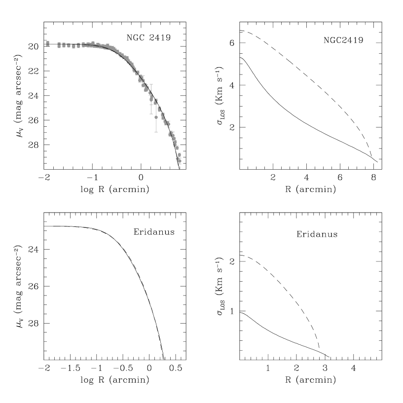
Figure 4: Surface-brightness (left panel) and LOS velocity-dispersion (right panel) profiles according to MOND (dashed lines) and Newtonian (solid lines) models for the globular clusters NGC2419 and Eridanus. The surface-brightness measures for NGC2419 from Trager et al. (1995) are overplotted in the upper left panel with grey points.

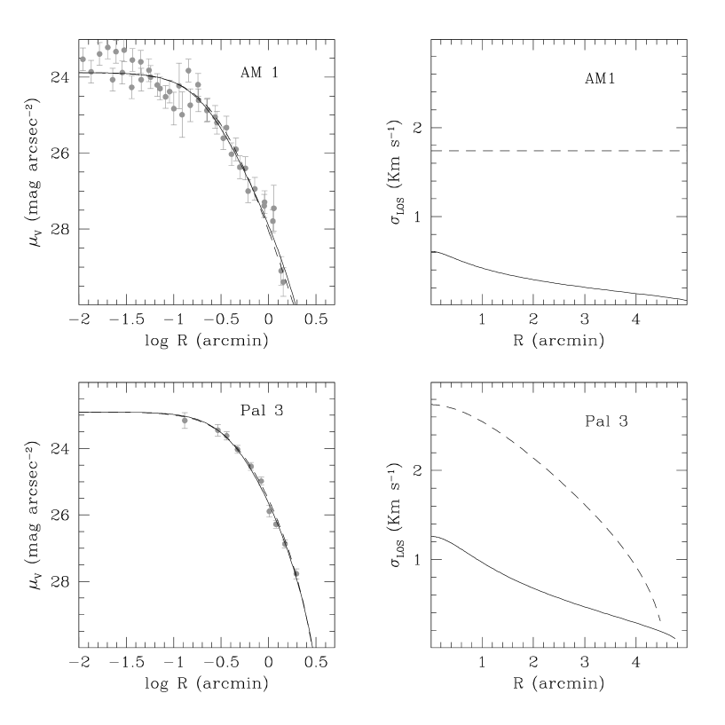
Figure 5: Same as Fig. 4, but for the globular clusters AM 1 and Pal 3.

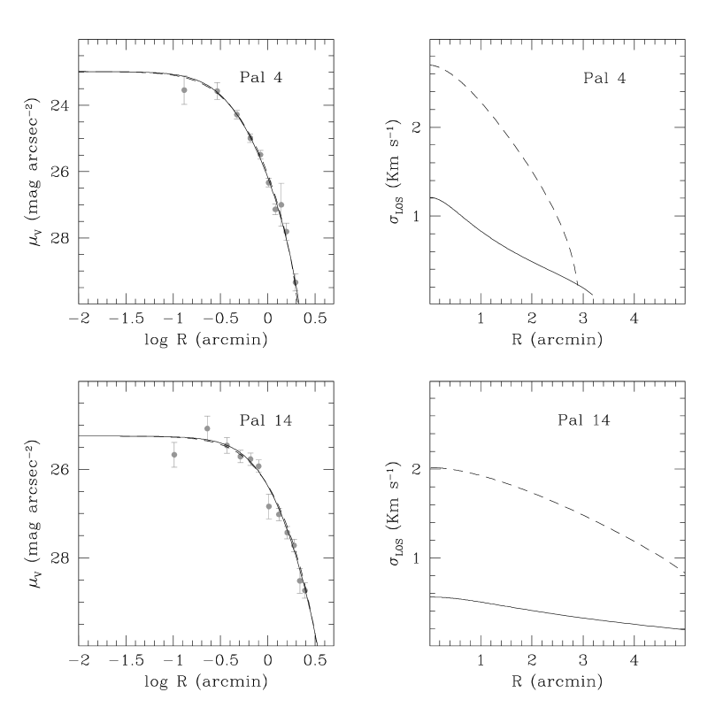
Figure 6: Same as Fig. 4, but for the globular clusters Pal 4 and Pal 14.

The examples shown in the previous Section suggest that the shape of the velocity-dispersion profile of a GC of given density profile can be quite different in MOND and Newtonian gravity. This makes the velocity-dispersion profiles of GCs a useful tool for distinguishing between MOND and Newtonian gravity. Here we apply our models to specific GCs, which may be used to test the MOND theory by combining measures of surface-brightness and LOS velocity-dispersion profiles. The models presented in this paper are valid in the external acceleration range $0<g_{\rm ext}\ll a_{0}$ (see Section 2.1). In spite of this limitation, a number of GCs belonging to the Galactic halo satisfy this constraint. Unfortunately, although the surface-brightness profiles of these clusters are well measured (McLaughlin & van der Marel 2005, hereafter MvdM05), to date none of them have accurate velocity-dispersion profiles. A first attempt at estimating the velocity-dispersion profile of NGC2419 has been done recently by Baumgardt et al. (2009).

Here we compare the velocity-dispersion profiles predicted by the Newtonian and MOND models that reproduce the surface-brightness profiles of six GCs located in the outer halo of the Milky Way (at distances $>50$ kpc from the Galactic centre). These clusters (listed in Table 1) are subject to an external Galactic acceleration $g_{\rm ext}{\mathrel{\mathchoice{\lower 2.9pt\vbox{\halign{$\m@th\displaystyle\hfil#\hfil$\cr<\crcr\sim\crcr}}}{\lower 2.9pt\vbox{\halign{$\m@th\textstyle\hfil#\hfil$\cr<\crcr\sim\crcr}}}{\lower 2.9pt\vbox{\halign{$\m@th\scriptstyle\hfil#\hfil$\cr<\crcr\sim\crcr}}}{\lower 2.9pt\vbox{\halign{$\m@th\scriptscriptstyle\hfil#\hfil$\cr<\crcr\sim\crcr}}}}}3\times 10^{-11}{\rm\,m\,s^{-1}}\ll a_{0}$, so they are fully in the regime of validity of our models.

3.1 MOND and Newtonian velocity-dispersion profiles for given mass and size

Though the masses and physical sizes of GCs are known only with non-negligible uncertainties, it is useful to discuss first the idealized case in which these quantities are given. In other words, for each object we fix a value of the mass-to-light ratio $M/L$ and of the cluster distance, valid for both Newtonian and MOND models, which is used to convert surface brightness in surface mass density. We defer to Section 3.2 a discussion of the effects of varying $M/L$ and distance. For Newtonian models we adopt the central dimensionless potentials $W_{0}$, core radii $r_{\rm c}$ and masses $M$ from MvdM05. For MOND models, we adopt the cluster mass estimated by MvdM05 and search for the values of $W_{0}$ and $\xi$ that best reproduce the surface-density profile of the corresponding Newtonian models.

In Table 1 the main structural properties derived for the six considered clusters are summarized. For Eridanus (which is not included in the catalog of MvdM05) we adopted the concentration, core radius, visual absolute magnitude given by Harris (1996) and estimated its mass by adopting a mass–V-band-luminosity ratio $M/L_{V}=1.892$ (the same value adopted by MvdM05 for Pal 4, which has similar age and metallicity; Catelan 2000). In both Newtonian and MOND cases, the central LOS velocity dispersion $\sigma_{\rm LOS,0}$ has been calculated by using equation (14).

Figures 4, 5 and 6 show the surface-brightness profiles (left panels) and velocity-dispersion profiles (right panels) of the Newtonian and MOND models of the six considered GCs. In the left panels we report also, where available, surface-brightness measures from Trager, King & Djorgovski (1995). As can be noted, MOND predictions significantly differ from Newtonian ones: in particular, it is apparent that the shape of MOND and Newtonian LOS velocity-dispersion profiles are remarkably different. As expected, MOND models predict a larger velocity dispersion along the entire cluster extent with respect to Newtonian models with the same mass. The physical reason at the basis of this result is that, as showed in Fig. 1, the same observed surface mass density profile is fitted by MOND models with a deeper potential well and larger core radii. As a consequence, at a given radius, the corresponding escape velocity is larger and according to equation (3) the width of the velocity distribution turns out to be larger. The same qualitative results have been obtained by Moffat & Toth (2008) and Haghi et al. (2009), who adopted different methods to calculate the velocity-dispersion profiles of the sample of GCs indicated by BGK05.

We note that the MOND $\sigma_{\rm LOS}$ profiles of our clusters are in general decreasing functions of radius and $\sigma_{\rm LOS}$ goes to zero when $r$ approaches the truncation radius, consistent with the fact that the no stars can cross the system’s boundary (see Sect. 2.2). An exception is the GC AM1, for which the predicted MOND velocity-dispersion profile in AM1 is flat along the entire cluster extent. The surface-brightness profile of this cluster is indeed well fitted by the MOND isothermal sphere model (Milgrom 1984) corresponding to its mass. The maximum difference in the velocity dispersion predicted by MOND and Newtonian theories ranges from $1.2{\rm\,km\,s^{-1}}$ (Eridanus) to $2.4{\rm\,km\,s^{-1}}$ (NGC2419), well above the accuracy currently achievable with high-resolution spectroscopic analyses.

Table 1: Structural parameters of the six considered outer halo globular clusters.

				Newtonian			MOND
Name	$\log(M/M_{\odot})$	$g_{\rm ext}/{a_{0}}$	$M/L_{V}$	$W_{0}$	$r_{\rm c}$	$\sigma_{\rm LOS,0}$	$W_{0}$	$\xi$	$\kappa$	$\sigma_{\rm LOS,0}$	$\Delta\sigma_{\rm LOS}^{max}$
			$M_{\odot}/L_{V,\odot}$		(pc)	$({\rm km}~{}{\rm s}^{-1})$				$({\rm km}~{}{\rm s}^{-1})$	$({\rm km}~{}{\rm s}^{-1})$
NGC2419	5.95	0.12	1.903	6.5	8.41	5.31	10.0	1.25	11.470	6.59	2.43
Eridanus	4.21	0.11	1.892	5.3	6.56	0.97	8.5	0.10	0.118	2.13	1.23
AM1	4.01	0.09	1.868	6.6	7.16	0.61	$\infty$	0.04	0.028	1.74	1.69
Pal 3	4.65	0.11	1.869	5.3	10.68	1.26	8.5	0.10	0.118	2.74	1.58
Pal 4	4.58	0.10	1.892	4.5	12.16	1.21	7	0.09	0.079	2.70	1.51
Pal 14	4.09	0.16	1.885	4.3	19.60	0.56	6.5	0.02	0.004	2.02	1.46

3.2 Dependence on mass-to-light ratio and distance

Figure 7: LOS velocity-dispersion profiles of a Newtonian King model with $W_{0}=6$ (solid line) compared with a family of MOND models with different values of $\kappa$, but with the same shape of the surface-brightness profile.

While the shape of the density and velocity-dispersion profiles of Newtonian King models does not depend on the structural parameters (mass and core radius), this is not the case for the corresponding MOND models. In these cases, the shape of the profiles varies for varying $r_{\rm c}$ and/or $M$. In other words, while Newtonian King models of given $W_{0}$ can be rescaled to represent systems of arbitrary values (in physical units) of $r_{\rm c}$ and $M$, a MOND model of given $W_{0}$ and $\xi$ represents only systems such that

$$\kappa\equiv\frac{GM}{a_{0}r_{\rm c}^{2}}=9\xi I(W_{0},\xi)$$ (21)

(see also Nipoti, Londrillo & Ciotti 2007c, for a detailed discussion of scaling of MOND models). For each value of $\kappa$ there is a unique pair of parameters ($W_{0},~{}\xi$) that reproduces a given shape of the surface-brightness profile. The shape of the corresponding velocity-dispersion profiles is different for different values of $\kappa$. This is illustrated in Fig. 7, where the velocity-dispersion profile of a Newtonian model with $W_{0}=6$ is compared with a family of MOND models that share the same surface-brightness profile, but have different values of $\kappa$. Here the LOS velocity dispersion and the radius are normalized to $\sigma_{\rm LOS,0}$ and $r_{\rm c}$ , respectively, to highlight the different shape of the profiles. It is evident that while small values of $\kappa$ produce steep profiles, the MOND profiles approach the Newtonian one for increasing $\kappa$. In fact, the larger $\kappa$ the larger the internal acceleration of the cluster, which eventually exceeds ${a_{0}}$ over most of the cluster extent.

In a practical application, once the surface-brightness profile of a given cluster is known, a unique pair of parameters ($W_{0},~{}\xi$) that reproduces the shape of the observed surface-brightness profile can be determined only when an estimate of $M$ and $r_{\rm c}$ is provided. On the other hand, the uncertainties on the mass-luminosity ratio and distance produce an uncertainty on $M$ and $r_{\rm c}$ and, consequently, on the predicted shape of the velocity-dispersion profile.

To illustrate this issue, in Fig. 8 we show the velocity-dispersion profiles of the models that reproduce the surface-brightness profile of NGC2419 assuming a different mass (central panel) and a different core radius (top panel). In particular, we let the cluster mass vary by $\Delta~{}\log\,(M/M_{\odot})=\pm 0.15$, with respect to the reference value $\log\,(M/M_{\odot})=5.95$ (therefore exploring the cases $M/L_{V}=2.7$ and $M/L_{V}=1.35$, beside the reference case $M/L_{V}=1.9$), and we let the cluster core radius vary by $\Delta~{}r_{\rm c}=\pm 0.1~{}r_{\rm c}$ (exploring the cases of cluster distance $d=81$ kpc and $d=99$ kpc, beside the reference case $d=90$ kpc). The corresponding overall cluster velocity dispersions (calculated by integrating $\sigma_{\rm LOS}$ over the entire cluster extent) are listed in Table 2. While a change in the core radius does not significantly affect either the shape or the central value of the velocity-dispersion profile, an even relatively small variation of $M$ significantly alters the overall value of the velocity dispersion.

It must be noted that even comparing the highest $M/L$ (and smallest distance) Newtonian model with the lowest $M/L$ (and larger distance) MOND model, the resulting LOS velocity-dispersion profiles are remarkably different and thus observationally distinguishable.

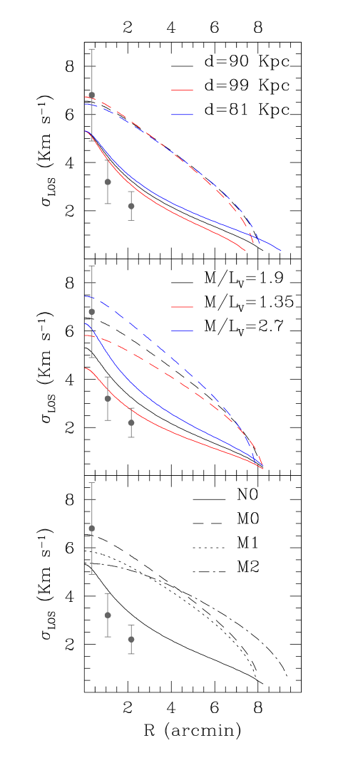
Figure 8: LOS velocity-dispersion profiles for NGC2419. In the top panel Newtonian models (solid lines) are compared with MOND models (dashed lines) with different assumptions on the cluster distance $d$. In the central panel Newtonian models (solid lines) are compared with MOND models (dashed lines) with different assumptions on the mass-to-light ratio. In the bottom panel the Newtonian model N0 (solid line) is compared with MOND models M0 (dashed line), M1 (dotted line) and M2 (dot-dashed line) differing in the choice of the interpolating function $\mu$ (see Table 2). The data by Baumgardt et al. (2009) are overplotted in the three panels.

3.3 Dependence on the interpolating function $\mu$

An additional uncertainty is related to the adopted form of the interpolating function $\mu$ (appearing in equation 1), which is not constrained theoretically, except for the asymptotic behaviour (see Section 1). The choice of the functional form of $\mu$ determines the behaviour of the MOND acceleration strength of the MOND effects in the intermediate acceleration regime (when $g$ is of the order of ${a_{0}}$), thus changing the overall shape of the velocity-dispersion profile.

In the bottom panel of Fig. 8 we show the velocity-dispersion profiles of the models that reproduce the surface-brightness profile of NGC2419 assuming different forms of the interpolating function $\mu$ (see Table 2), but keeping fixed $M$ and $r_{\rm c}$. As expected, both the morphology of the velocity-dispersion profile and its average value depend on $\mu$. However, the effect of varying $\mu$ is typically small if we limit ourselves to standard proposal such as equation (16) (model M0) or Milgrom’s (1983) $\mu(y)=y/\sqrt{1+y^{2}}$ (model M1), and we exclude unrealistic cases such as the step function adopted in model M2.

3.4 Comparison with velocity-dispersion measures

Table 2: Predicted overall velocity dispersion for different MOND and Newtonian models of NGC2419.

Model	$\mu(y)$	$\log\,(M/M_{\odot})$	$r_{\rm c}$	$<\sigma_{\rm LOS}>$
			(pc)	$({\rm\,km\,s^{-1}})$
N0	1	5.95	8.41	4.40
Nm-	1	5.80	8.41	3.70
Nm+	1	6.10	8.41	5.23
Nr-	1	5.95	7.57	4.64
Nr+	1	5.95	9.25	4.20
M0	$y/(1+y)$	5.95	9.50	6.18
M1	$y/\sqrt{1+y^{2}}$	5.95	8.50	5.56
M2	$\max(y,1)$	5.95	7.96	5.22
Mm-	$y/(1+y)$	5.80	10.28	5.51
Mm+	$y/(1+y)$	6.10	9.23	6.93
Mr-	$y/(1+y)$	5.95	8.54	6.28
Mr+	$y/(1+y)$	5.95	11.08	6.07

We have seen that, at least for the representative case of NGC2419, while the same overall velocity dispersion can be predicted by both Newtonian and MOND models with different choices of the mass-to-light ratio or of the interpolating function (compare, e.g., model Nm+ with models M1, M2, and Mm- in Table 2), MOND profiles can be always easily distinguished from Newtonian ones. The analysis of the shape of the velocity-dispersion profile represents therefore a robust method to discriminate between the two gravity theories. This method is indeed less sensitive to the errors on the cluster mass with respect to the simple comparison between the overall cluster velocity dispersion proposed by BGK05. Moreover, the approach suggested by these authors favours low-mass GCs whose internal acceleration is lower than ${a_{0}}$ at any distance from the cluster centre. The low mass of these clusters, together with their large distances, imply a poor efficiency in measuring radial velocities for a meaningful sample of stars.

Of course, measuring the velocity-dispersion profile is observationally more challenging than estimating the overall velocity dispersion, but these kinds of measures are becoming feasible even for relatively distant GCs. In Fig. 8 we overplot the three velocity-dispersion measures obtained by Baumgardt et al. (2009) from spectroscopic observations of 40 stars of NGC2419. Though there are large uncertainties due to the poor statistics, the overall trend defined by these observations appears hard to reconcile with MOND, at least under the considered assumption of spherical symmetry and isotropic velocity distribution. This preliminary result confirms that NGC 2419 might be a crucial object to test MOND (as also suggested by Baumgardt et al. 2009) and strongly encourages future studies of this object combining higher resolution observations of a larger number of stars of NGC2419 as well as a systematic study of the possible effects of orbital anisotropy, rotation and deviation from spherical symmetry. Among these effects, that of orbital anisotropy is likely the most important, because the shape of the LOS velocity-dispersion profile can depend significantly on the distribution of stellar orbits. In particular, a radially anisotropic system is expected to have centrally steeper $\sigma_{\rm LOS}$ profile than an isotropic system with the same spatial distribution. Therefore, it is worth investigating whether radially anisotropic MOND models can be reconciled with the velocity dispersion data for NGC2419. We address this question in the next Section.

3.5 Radially anisotropic models of NGC2419

Ideally, to explore the effect of orbital anisotropy on the $\sigma_{\rm LOS}$ profiles of GCs, one would need self-consistent anisotropic MOND models derived from the distribution function. Constructing such models is beyond the purpose of the present work: here we perform a preliminary analysis based on the numerical integration of the Jeans equations. We follow the standard procedure (Binney & Mamon 1982), but with the MOND gravitational field replacing the Newtonian field. In practice, we take the spherically symmetric density distribution of the King model of NGC2419 (parameters in Table 1), rescale it for the assumed value of $M/L_{V}$, and compute the MOND field generated by this density distribution using equation (2). We then solve the Jeans equations assuming an anisotropy-parameter profile $\beta(r)\equiv 1-\sigma^{2}_{\rm t}(r)/2\sigma^{2}_{r}(r)$, where $\sigma^{2}_{\rm t}$ and $\sigma^{2}_{r}$ are the tangential and radial components of the velocity dispersion tensor. Finally, we obtain the $\sigma_{\rm LOS}(r)$ by deprojecting $\sigma^{2}_{r}(r)$. For comparison, we also obtain $\sigma_{\rm LOS}$ profiles of anisotropic Newtonian models using the same procedure.

As stressed in the Introduction, the Jeans-equations approach does not guarantee that the obtained models are self-consistent. However, we can at least use some necessary conditions for consistency (e.g., Ciotti & Pellegrini 1992; An & Evans 2006; Ciotti & Morganti 2009) to exclude unphysical $\beta(r)$. We note that these necessary conditions, though derived in the context of Newtonian gravity, apply to our self-gravitating MOND models, because each of this models can be formally interpreted as a non-self-gravitating distribution of tracer stars in the presence of a dominant mass distribution having the same gravitational potential as the MOND potential of the cluster. An & Evans (2006) show that a necessary condition for consistency is $\beta(0)\leq\gamma/2$, where $\gamma\equiv-\lim_{r\to 0}d\ln\rho/{\rm d}\ln r$ is the central logarithmic slope of the stellar density distribution. For NGC2419 $\gamma\sim 0$, so models with $\beta(0){\mathrel{\mathchoice{\lower 2.9pt\vbox{\halign{$\m@th\displaystyle\hfil#\hfil$\cr>\crcr\sim\crcr}}}{\lower 2.9pt\vbox{\halign{$\m@th\textstyle\hfil#\hfil$\cr>\crcr\sim\crcr}}}{\lower 2.9pt\vbox{\halign{$\m@th\scriptstyle\hfil#\hfil$\cr>\crcr\sim\crcr}}}{\lower 2.9pt\vbox{\halign{$\m@th\scriptscriptstyle\hfil#\hfil$\cr>\crcr\sim\crcr}}}}}0$ are inconsistent, implying that spherical, radially anisotropic models with $\beta$ independent of radius are unphysical. We then consider Osipkov-Merritt (hereafter OM) models (Ospikov 1979; Merritt 1985), which are isotropic in the centre and radially anisotropic at large radii, having

$$\beta(r)={r^{2}\over r^{2}+r_{\rm a}^{2}},$$ (22)

where $r_{\rm a}$ is the anisotropy radius. A necessary condition for the consistency of OM models is that $(r^{2}+r_{\rm a}^{2})\rho(r)$ is a non-increasing function of radius (Ciotti & Pellegrini 1992). In the considered model of NGC2419 this condition is satisfied for $r_{\rm a}{\mathrel{\mathchoice{\lower 2.9pt\vbox{\halign{$\m@th\displaystyle\hfil#\hfil$\cr>\crcr\sim\crcr}}}{\lower 2.9pt\vbox{\halign{$\m@th\textstyle\hfil#\hfil$\cr>\crcr\sim\crcr}}}{\lower 2.9pt\vbox{\halign{$\m@th\scriptstyle\hfil#\hfil$\cr>\crcr\sim\crcr}}}{\lower 2.9pt\vbox{\halign{$\m@th\scriptscriptstyle\hfil#\hfil$\cr>\crcr\sim\crcr}}}}}9.43\,{\rm pc}\simeq 1.12r_{\rm c}$, where $r_{\rm c}$ is the core radius given in Table 1. In Fig. 9 we plot the $\sigma_{\rm LOS}$ profile for maximally radially anisotropic ($r_{\rm a}=1.12r_{\rm c}$) MOND and Newtonian OM models of NGC2419 for the three reference values of $M/L_{V}$ adopted in Fig. 8: as expected, radially anisotropic models predict higher $\sigma_{\rm LOS}$ in the centre and lower $\sigma_{\rm LOS}$ in the outer regions than the corresponding isotropic models (middle panel in Fig. 8). While radially anisotropic Newtonian models reproduce well the observational data from Baumgardt et al. (2009), MOND anisotropic models still tend to predict too high velocity dispersion.

Given the large uncertainties in the observational data, it is not excluded that the velocity-dispersion profile of NGC2419 can be reproduced by a MOND radially anisotropic model with low stellar mass-to-light ratio. However, it must be stressed that the models plotted in Fig. 9 are extreme cases: they satisfy only the necessary condition for consistency, so they may have to be excluded as unphysical or unstable.

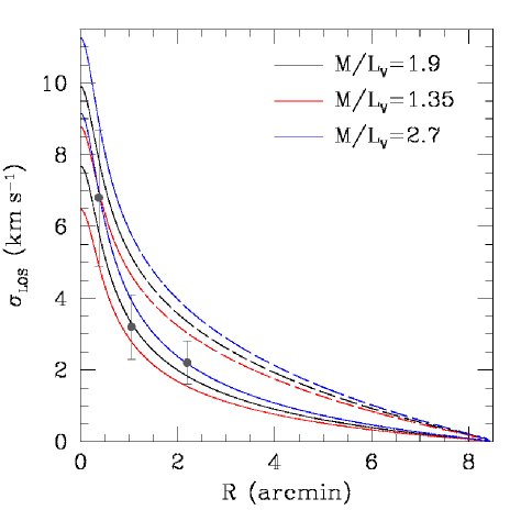
Figure 9: Same as the middle panel of Fig. 8, but for radially anisotropic (Osipkov-Merritt) Newtonian (solid lines) and MOND (dashed lines) models of NGC2419.

4 Summary and conclusions

We have presented self-consistent dynamical models of stellar systems in MOND that can be used to study GCs in the outer Galactic regions. These models, which are the analogues of the Newtonian King models, are able to reproduce the observed surface-brightness profiles of GCs and can be used to predict their projected velocity-dispersion profiles in MOND. By comparing our models with the corresponding Newtonian ones, we found that it is impossible to reproduce simultaneously the same density and velocity-dispersion profiles with both gravitational theories regardless of any choice of the free parameters of the models. This indicates GCs are one of the best laboratories to test the gravity theory in the low-acceleration regime, as already suggested by various authors (Scarpa, Marconi & Gilmozzi 2003; BGK05; Scarpa et al. 2007; Moffat & Toth 2008; Haghi et al. 2009; Lane et al. 2009).

Of course, the same effect produced by MOND on the velocity-dispersion profile can by reproduced by an $ad~{}hoc$ distribution of dark matter. The presence of dark-matter halos in GCs is predicted by some theories of GC formation and evolution (see Mashchenko & Sills 2005 and references therein) and its observational evidence is still matter of debate (Moore 1996; Forbes et al. 2008). Thus, the detection of velocity-dispersion profiles in agreement with the predictions of MOND would not necessarily be a problem for the dark-matter paradigm. On the other hand, it must be stressed that the detection of velocity-dispersion profiles expected on the basis of Newtonian dynamics (without dark matter) could invalidate MOND.

Testing MOND by using nearby GCs has been already attempted by Scarpa et al. (2003) who found that their velocity-dispersion profiles deviate from the prediction of Newtonian dynamics (without dark matter) at large distance from their centres. However, the nearby clusters analysed by these authors experience an external acceleration due to the Milky Way gravitational field that is larger than the critical acceleration $a_{0}$ (BGK05; Moffat & Toth 2008). BGK05 indicated a sample of eight GCs where the predictions of MOND and Newtonian theories on the overall LOS velocity dispersion significantly differ. However, the method proposed by these authors is very sensitive to the adopted mass and distance of these clusters. Given the large distances and low mass of these clusters, it is very difficult to observe the significant number of cluster member stars necessary to an accurate estimate of the velocity dispersion. In this regard, the difference between the MOND and Newtonian predictions estimated by these authors never exceeds $\Delta\sigma_{\rm LOS}<1.3{\rm\,km\,s^{-1}}$. Given the best accuracy achievable by the current observing facilities ($\sim 0.5{\rm\,km\,s^{-1}}$), it is hard to reach a firm conclusion on the validity of MOND using this approach. Nevertheless, the first results of the application of this method to Pal 14 suggests that the observed kinematic of this system might be a problem for MOND (Jordi et al. 2009).

A more robust test is to compare the observed shape of the velocity-dispersion profile with the prediction of Newtonian and MOND models (see also Moffat & Toth 2008; Haghi et al. 2009). We demonstrated that this method always allows an unambiguous distinction between Newtonian and MOND scenarios even when large uncertainties on the cluster mass and core radii are present. The best target GC, for which this approach is expected to be particularly efficient, is NGC2419. Indeed, although not included in the list of BGK05, this cluster is the one with the largest absolute difference in the predicted velocity-dispersion profile by Newtonian and MOND models. Moreover, it is not significantly affected by Galactic tidal effects (Gnedin & Ostriker 1999) that can alter the shape of the velocity-dispersion profile in the outermost regions (Johnston, Sigurdsson & Hernquist 1999) and is massive enough to ensure a large number of stars at magnitudes easily reachable by the current generation of spectrographs. Recently Baumgardt et al. (2009) measured the velocity dispersion at three different radii in this cluster. The two outermost data points are significantly lower than the velocity-dispersion profiles predicted by our isotropic MOND models of NGC2419, at least for stellar mass-to-light ratios in the range $1.35{\mathrel{\mathchoice{\lower 2.9pt\vbox{\halign{$\m@th\displaystyle\hfil#\hfil$\cr<\crcr\sim\crcr}}}{\lower 2.9pt\vbox{\halign{$\m@th\textstyle\hfil#\hfil$\cr<\crcr\sim\crcr}}}{\lower 2.9pt\vbox{\halign{$\m@th\scriptstyle\hfil#\hfil$\cr<\crcr\sim\crcr}}}{\lower 2.9pt\vbox{\halign{$\m@th\scriptscriptstyle\hfil#\hfil$\cr<\crcr\sim\crcr}}}}}M/L_{V}{\mathrel{\mathchoice{\lower 2.9pt\vbox{\halign{$\m@th\displaystyle\hfil#\hfil$\cr<\crcr\sim\crcr}}}{\lower 2.9pt\vbox{\halign{$\m@th\textstyle\hfil#\hfil$\cr<\crcr\sim\crcr}}}{\lower 2.9pt\vbox{\halign{$\m@th\scriptstyle\hfil#\hfil$\cr<\crcr\sim\crcr}}}{\lower 2.9pt\vbox{\halign{$\m@th\scriptscriptstyle\hfil#\hfil$\cr<\crcr\sim\crcr}}}}}2.7$. Only assuming quite strong radial orbital anisotropy and lower stellar mass-to-light ratio the velocity dispersion predicted by MOND can be reconciled with the observed data of NGC2419. Reproducing the observed kinematics of NGC2419 represents a challenge for MOND, although better data sets (larger number of stars and higher spectral resolution) and more sophisticated modelling are needed.

A limitation of the present study is that our models are spherically symmetric, non rotating and with isotropic velocity distribution. The assumption of spherical symmetry and absence of significant rotation is in general justified by the round appearance of GCs. In general, non-sphericity can be a problem in the determination of surface brightness and velocity dispersion profiles when large ellipticities are present (Perina et al. 2009). This effect should have only a minor impact in GCs which have generally symmetric density contours, at least within few core radii. The amount of anisotropy in many GCs is estimated to be relatively small (Ashurov & Nuritdinov 2001), though a non-negligible degree of anisotropy is likely to be present in few GCs (Meylan & Heggie 1997 and references therein). Orbital anisotropy is also predicted by N-body simulations as a result of both primordial and evolutionary reasons (Giersz 2006). These effects are expected to be at least partially erased in Galactic GCs by the strong tidal interaction with the Milky Way which removes the initial velocity anisotropies and angular momentum making them more spherical (Goodwin 1997). A preliminary exploration of the effects of an extreme radial anisotropy shows a significant degeneracy between gravity law and orbital anisotropy. Nevertheless, the MOND and Newtonian models can be distinguished when high precision data are available. Another possible complication can be due to the presence of a significant fraction of unresolved binaries which can inflate the observed velocity dispersions (Cote et al. 2002). For instance, in NGC2419 the orbital velocity of a pair of equal-mass 0.8 $M_{\odot}$ stars separated by $a\leq 14~{}AU$ could be as high as 10 $Km~{}s^{-1}$, remaining stable against collisional disruption (Hills 1984). A significant fraction of binaries can therefore increase the observed velocity dispersion by few $Km~{}s^{-1}$. This effect is particularly important in the central part of the cluster where binaries preferentially sink as a result of mass segregation. This could explain why the measured central velocity dispersion in NGC2419 seems higher than the prediction of both Newtonian and MOND models. Note however that, in the case of NGC2419, the ”binary-corrected” velocity dispersion would stray even more from the prediction of MOND models in the external region of the cluster. Given these uncertainties, a systematic exploration of the effects on the cluster kinematics of orbital anisotropy, rotation and deviation from spherical symmetry in general would be valuable also in MOND as well as in Newtonian dynamics (see Bertin & Varri 2008, and references therein).

Appendix A Numerical integration

We describe briefly the procedure used to numerically integrate equation (13), from $\tilde{r}=0$ to a given radius $\tilde{r}$, to obtain $W(\tilde{r})$. Equation (13) can be written as

$$\left[\frac{2}{\tilde{r}}\frac{{\rm d}W}{{\rm d}\tilde{r}}+\frac{{\rm d}^{2}W}{{\rm d}\tilde{r}^{2}}\right]\mu\left(\xi\left|{{\rm d}W\over{\rm d}\tilde{r}}\right|\right)-\frac{{\rm d}W}{{\rm d}\tilde{r}}\xi\frac{{\rm d}^{2}W}{{\rm d}\tilde{r}^{2}}\mu^{\prime}\left(\xi\left|{{\rm d}W\over{\rm d}\tilde{r}}\right|\right)=-9\tilde{\rho}$$ (23)

where

$$\mu^{\prime}(y)\equiv\frac{d\mu(y)}{dy}.$$ (24)

The term ${\rm d}^{2}W/{\rm d}\tilde{r}^{2}$ diverges at the centre, but, for any choice of the MOND interpolating function $\mu$, substitutions of power series show that

$$\lim_{\tilde{r}\rightarrow 0}\frac{{\rm d}^{2}W}{{\rm d}\tilde{r}^{2}}=-\sqrt{\frac{3}{4\xi}}\tilde{r}^{-\frac{1}{2}}$$ (25)

whose integral converges and admits the exact solution

$$\left.\frac{{\rm d}W}{{\rm d}\tilde{r}}\right|_{\tilde{r}\rightarrow 0}=-\sqrt{\frac{3}{\xi}}\tilde{r}^{\frac{1}{2}},$$

$$W|_{\tilde{r}\rightarrow 0}=W_{0}-\sqrt{\frac{4}{3\xi}}\tilde{r}^{\frac{3}{2}}.$$

We used the above equations to calculate the dimensionless potential and its derivatives at the centre. For the subsequent integration steps we adopted a radial step $\Delta\tilde{r}$ such that

$$\max\left(\frac{{\rm d}W}{{\rm d}\tilde{r}}\Delta\tilde{r},\frac{{\rm d}^{2}W}{{\rm d}\tilde{r}^{2}}\Delta\tilde{r}\right)<0.01,$$ (26)

in order to ensure a negligible numerical error in the integrations.

References

- An & Evans (2006) An J.H., Evans N.W., 2006, ApJ, 642, 752
- Angus (2008) Angus G. W., 2008, MNRAS, 387, 1481
- Angus et al. (2007) Angus G. W., Shan H. Y., Zhao H. S., Famaey B., 2007, ApJ, 654, L13
- Angus & Diaferio (2009) Angus G. W., Diaferio A., 2009, MNRAS, 396, 887
- Ashurov & Nuritdinov (2001) Ashurov A., Nuritdinov S., 2001, in Deiters S., Fuchs B., Sprutzem R., Just A., Wielen R., eds., Dynamics of Star Clusters and the Milky Way, 228, 371
- Baumgardt et al. (2005) Baumgardt H., Grebel E. K., Kroupa P., 2005, MNRAS, 359, L1 (BGK05)
- Baumgardt et al. (2009) Baumgardt H., Côté P., Hilker M., Rejkuba M., Mieske S., Djorgovski S. G., Stetson P., 2009, MNRAS, 396, 2051
- Bekenstein (2006) Bekenstein J., 2006, ConPh, 47, 387
- Bekenstein (2009) Bekenstein J. D., 2009, NuPhA, 827, 555
- Bekenstein & Milgrom (1984) Bekenstein J., Milgrom M., 1984, ApJ, 286, 7
- Bertin & Varri (2008) Bertin G., Varri A. L., 2008, ApJ, 689, 1005
- Bienaymé et al. (2009) Bienaymé O., Famaey B., Wu X., Zhao H. S., Aubert D., 2009, A&A, 500, 801
- Binney & Mamon (1982) Binney J., Mamon G.A., 1982, MNRAS, 200, 361
- Brada & Milgrom (2000) Brada R., Milgrom M., 2000, ApJ, 541, 556
- Catelan (2000) Catelan M., 2000, ApJ, 531, 826
- Ciotti, Londrillo, & Nipoti (2006) Ciotti L., Londrillo P., Nipoti C., 2006, ApJ, 640, 741
- Ciotti & Pellegrini (1992) Ciotti L., Pellegrini S., 1992, MNRAS, 255, 561
- Ciotti & Morganti (2009) Ciotti L., Morganti L., 2009, MNRAS, 393, 179
- Clowe et al. (2006) Clowe D., Bradač M., Gonzalez A. H., Markevitch M., Randall S. W., Jones C., Zaritsky D., 2006, ApJ, 648, L109
- Côté et al. (2002) Côté P., Djorgovski S. G., Meylan G., Castro S., McCarthy J. K., 2002, ApJ, 574, 783
- Evans, An & Walker (2009) Evans N.W., An J.H., Walker M.G., 2009, MNRAS, 393, L50
- Famaey & Binney (2005) Famaey B., Binney J., 2005, MNRAS, 363, 603
- Forbes et al. (2008) Forbes D. A., Lasky P., Graham A. W., Spitler L., 2008, MNRAS, 389, 1924
- Giersz (2006) Giersz M., 2006, MNRAS, 371, 484
- Gnedin & Ostriker (1999) Gnedin O. Y., Ostriker J. P., 1999, ApJ, 513, 626
- Goodwin (1997) Goodwin S. P., 1997, MNRAS, 286, L39
- Haghi et al. (2009) Haghi H., Baumgardt H., Kroupa P., Grebel E. K., Hilker M., Jordi K., 2009, MNRAS, 395, 1549
- Harris (1996) Harris W. E., 1996, AJ, 112, 1487
- Hills (1984) Hills J. G., 1984, AJ, 89, 1811
- Johnston et al. (1999) Johnston K. V., Sigurdsson S., Hernquist L., 1999, MNRAS, 302, 771
- Jordi et al. (2009) Jordi K., et al., 2009, AJ, 137, 4586
- King (1966) King I. R., 1966, AJ, 71, 64
- Kleyna et al. (2001) Kleyna J. T., Wilkinson M. I., Evans N. W., Gilmore G., 2001, ApJ, 563, L115
- Lane et al. (2009) Lane R. R., Kiss L. L., Lewis G. F., Ibata R. A., Siebert A., Bedding T. R., Székely P., 2009, arXiv, arXiv:0908.0770
- Londrillo & Nipoti (2009) Londrillo P., Nipoti C., 2009, MSAIS, 13, 89
- Mashcenko & Sills (2005) Mashchenko S., Sills A., 2005, ApJ, 619, 243
- McLaughlin & van der Marel (2005) McLaughlin D. E., van der Marel R. P., 2005, ApJS, 161, 304 (MvdM05)
- Meylan & Heggie (1997) Meylan G., Heggie D. C., 1997, A&ARv, 8, 1
- Merritt (1985) Merritt D., 1985, AJ, 90, 102
- Milgrom (1983) Milgrom M., 1983, ApJ, 270, 365
- Milgrom (1984) Milgrom M., 1984, ApJ, 287, 571
- Milgrom (2008) Milgrom M., 2008, in Matter and Energy in the Universe: From Nucleosynthesis to Cosmology. XIX Rencontres de Blois, arXiv:0801.3133
- Milgrom & Bekenstein (1987) Milgrom M., Bekenstein J., 1987, in Dark matter in the universe, D. Reidel Publishing Co., Dordrecht, 117, 319
- Moffat & Toth (2008) Moffat J. W., Toth V. T., 2008, ApJ, 680, 1158
- Moore (1996) Moore B., 1996, ApJ, 461, L13
- Natarajan & Zhao (2008) Natarajan P., Zhao H., 2008, MNRAS, 389, 250
- Nipoti, Londrillo & Ciotti (2007) Nipoti C., Londrillo P., Ciotti L., 2007a, MNRAS, 381, L104
- Nipoti et al. (2007b) Nipoti C., Londrillo P., Zhao H.S., Ciotti L., 2007b, MNRAS, 379, 597
- Nipoti, Londrillo, & Ciotti (2007c) Nipoti C., Londrillo P., Ciotti L., 2007c, ApJ, 660, 256
- Nipoti et al. (2008) Nipoti C., Ciotti L., Binney J., Londrillo P., 2008, MNRAS, 386, 2194
- Osipkov (1979) Osipkov L.P., 1979, Soviet Astron. Lett., 5, 42
- Perina et al. (2009) Perina S., et al., 2009, A&A, 494, 933
- Sánchez-Salcedo, Reyes-Iturbide & Hernandez (2006) Sánchez-Salcedo F.J., Reyes-Iturbide J., Hernandez X., 2006, 370, 1829
- Sánchez-Salcedo & Hernandez (2007) Sánchez-Salcedo F. J., Hernandez X., 2007, ApJ, 667, 878
- Sanders (2007) Sanders R. H., 2007, MNRAS, 380, 331
- Sanders & McGaugh (2002) Sanders R. H., McGaugh S. S., 2002, ARA&A, 40, 263
- Scarpa et al. (2003) Scarpa R., Marconi G., Gilmozzi R., 2003, A&A, 405, L15
- Scarpa et al. (2007) Scarpa R., Marconi G., Gilmozzi R., Carraro G., 2007, A&A, 462, L9
- The & White (1988) The L. S., White S. D. M., 1988, AJ, 95, 1642
- Trager et al. (1995) Trager S. C., King I. R., Djorgovski S., 1995, AJ, 109, 218
- Wu et al. (2008) Wu X., Famaey B., Gentile G., Perets H., Zhao H., 2008, MNRAS, 386, 2199
- Wu et al. (2007) Wu X., Zhao H., Famaey B., Gentile G., Tiret O., Combes F., Angus G. W., Robin A. C., 2007, ApJ, 665, L101