Hybrid-functional calculations with plane-wave basis sets: The effect of the singularity correction on total energies, energy eigenvalues, and defect energy levels

Abstract

When described through a plane-wave basis set, the inclusion of exact nonlocal exchange in hybrid functionals gives rise to a singularity, which slows down the convergence with the density of sampled $k$ points in reciprocal space. In this work, we investigate to what extent the treatment of the singularity through the use of an auxiliary function is effective for $k$-point samplings of limited density, in comparison to analogous calculations performed with semilocal density functionals. Our analysis applies for instance to calculations in which the Brillouin zone is sampled at the sole $\Gamma$-point, as often occurs in the study of surfaces, interfaces, and defects or in molecular dynamics simulations. In the adopted formulation, the treatment of the singularity results in the addition of a correction term to the total energy. The energy eigenvalue spectrum is affected by a downwards shift of the energy eigenvalues of the occupied states, while those of the unoccupied states remain unaffected. Analogous corrections also speed up the convergence of screened exchange interactions despite the absence of a proper singularity. Focusing first on neutral systems, both finite and extended, we show that the account of the singularity corrections bears convergence properties which are quantitatively similar to those observed with semilocal density functionals. We emphasize that this is not the case for uncorrected energies, particularly for elongated simulation cells for which qualitatively different trends are found. We then consider differences between total energies of systems differing by their charge state. For systems involving localized electron states, such as ionization potentials and electron affinities of molecular systems or charge transition levels of point defects, the proper account of the singularity correction yields convergence properties which are similar to those of neutral systems. In the case of extended systems, such energy differences provide an alternative way to determine the band edges, but are found to converge more slowly with simulation cell than in corresponding semilocal functionals because of the exchange selfinteraction associated to the extra charge.

I Introduction

In the past decades, density functional theoryHohenberg_PR_1964 ; Kohn_PR_1965 has become the mainstream technique for electronic structure calculations of large molecules, clusters, liquids, and solids. In condensed matter applications, the most common functional has initially been based on the local density approximation (LDA),Kohn_PR_1965 but generalized gradient approximations have become increasingly popular in the last two decades.Perdew_PRB_1986 ; Becke_JCP_1986 ; Becke_PRA_1988 ; Perdew_PRB_1992 ; Perdew_PRL_1996 A class of functionals that could potentially lead to higher accuracy include a fraction of exact nonlocal exchange in the exchange-correlation potential.Becke_JCP_1993a ; Becke_JCP_1993b This class of functionals, referred to as hybrid functionals, has become the standard electronic-structure approach in quantum-chemistry applications. For molecular systems, these functionals achieve a more accurate description not only of atomization energies,Curtiss_JCP_1997 but also of ionization potentials and electron affinities.Curtiss_JCP_1998 However, several shortcomings still remain. For instance, the desired chemical accuracy is not always attained and no solution is offered for the treatment of Van-der-Waals interactions. Nevertheless, it appears quite clearly that the inclusion of exact exchange constitutes an improvement, which might be particularly useful in several circumstances.

When applied to semiconductors and insulators, hybrid functionals provide a superior description to semilocal functionals. For instance, structural parameters are found to be closer to experimental values.Heyd_JCP_2005 ; Paier_JCP_2006 Furthermore, hybrid functionals give electronic band gaps which are systematically larger than those achieved with semilocal functionals, generally leading to a better agreement with experiment.Muscat_CPL_2001 ; Heyd_JCP_2005 ; Paier_JCP_2006 In particular, the improvement achieved by hybrid functionals in which the Coulomb potential is screened is remarkable,Heyd_JCP_2005 ; Paier_JCP_2006 and the origin of this successful description can be rationalized.Janesko_PCCP_2009 A more accurate description of the band gap is especially important in certain classes of problems, such as the study of surface and interface statesPaier_JCP_2005 ; DiValentin_PRL_2006 and the determination of defect energy levels.VanDeWalle_JAP_2004 Indeed, a physically meaningful description of electronic states lying in the band gap can only be achieved when the calculated band gap approaches the experimental one.VanDeWalle_JAP_2004 ; Pacchioni_PRB_2000 ; Zhang_PRB_2001 ; Knaup_PRB_2005 ; Deak_JPCM_2005 ; Xiong_APL_2005 ; Gavartin_APL_2006 ; Broqvist_APL_2006 ; DiValentin_PRL_2006 ; Lany_PRL_2007 ; Janotti_PRB_2007 ; Broqvist_APL_2008 ; Alkauskas_PRL_2008 ; Broqvist_PRB_2008 ; Paudel_PRB_2008 ; Oba_PRB_2008 ; Alkauskas_PRB_2008 ; Lany_PRB_2008

For the treatment of condensed systems, hybrid functionals have been available for some time in codes combining Gaussian basis sets and periodic boundary conditions.Pisani_IJQC_1980 ; Gaussian03 However, it is expected that the treatment of the electronic structure through hybrid functionals carries potential to be much more widely used in an implementation based on plane-wave basis sets and pseudopotentials.Payne_RMP_1992 In this respect, the treatment of exact exchange poses several new problems with respect to the use of standard semilocal functionals.

First, the calculation of exact exchange entails a significantly higher computational cost. To address this issue, efficient algorithms have been developed to optimize the scaling with respect to the number of plane waves.Chawla_JCP_1998 ; Sorouri_JCP_2006 ; Todorova_JPCB_2006 A further gain is achieved through optimal adaptation to new massively parallel computer platforms.CPMD Despite these improvements, plane-wave based hybrid-functional calculations for a system of 1000 electrons still yield a computational cost exceeding that of semilocal ones by more than two orders of magnitude.Broqvist_APL_2008 ; Alkauskas_PRL_2008b Nevertheless, such calculations are attracting increasing interest as larger computational resources become available.

Second, the expression for exact exchange includes an integrable divergence,Kittel_1963 which hinders its straightforward use within plane-wave formulations because of its slow convergence with the density of $k$ points. Gygi and Baldereschi proposed a numerical treatment of the divergence based on the analytic integration of an auxiliary function showing the same singularity.Gygi_PRB_1986 Such auxiliary functions are nowadays available for arbitrary unit cells.Massidda_PRB_1993 ; Sorouri_JCP_2006 ; Carrier_PRB_2007 Alternative treatments consist in truncating the Coulomb operator,Spencer_PRB_2008 using a screened Coulomb potential,Todorova_JPCB_2006 or transforming the Bloch functions in order to compute real-space Coulomb integrals.Wu_PRB_2009

Third, the nonlocal exchange coupling between valence and core states also intervenes in the basic pseudopotential approximation. Such interactions can be accounted for within an all-electron scheme in which the pseudopotential approximation consists in freezing the wave functions of the core states.Paier_JCP_2005 The core-valence interactions due to exchange then lead to a modification of the nonlocal pseudopotential term. In consideration of the fact that current hybrid functionals generally only include a fraction of exact exchange (about 25%), pseudopotentials derived within semilocal formulations have often been transferred to hybrid schemes without any modificationTodorova_JPCB_2006 ; Wang_JACS_2007 ; Broqvist_APL_2008 ; Alkauskas_PRL_2008 or through the only use of nonlinear core corrections.Broqvist_PRB_2008 However, when core-valence interactions are sizable, these practices require particular care, and it has recently been pointed out that they might lead to inconsistencies.Stroppa_NJP_2008

In this work, we focus specifically on aspects associated with the treatment of the integrable singularity when calculating the exact exchange expresssion in electronic-structure schemes based on plane-wave basis sets. Following Gygi and Baldereschi,Gygi_PRB_1986 we adopt a formulation in which the divergence is treated analytically. This scheme can be recast in such a way that the treatment of the divergence results in a correction term formally corresponding to the Fourier component of the exchange potential at vanishing wavevector in the Brillouin zone.Carrier_PRB_2007 We first address the degree of convergence that can be achieved with a $k$-point sampling of finite density for both the total energy and the energy eigenvalues, in comparison with a similar calculation that does not include exact exchange. This aspect is particularly important to validate calculations based on large simulations cells with the Brillouin zone sampled only at the $\Gamma$ point, a configuration which is often used in surface, interface, and defect calculations or in ab initio molecular dynamics simulations. We also consider exchange interactions based on screened Coulomb potentials. While this case formally does not show a singularity, there are specific circumstances in which the same convergence deficiency occurs as for the bare Coulomb potential. We then study the effect of the singularity correction on the total energy of charged systems. Differences between total energies of systems involving a different number of electrons are relevant for determining the electron affinity, the ionization potential, the band gap, and the charge transition levels of defects. We discuss the effect of the correction on these quantities for the cases of both finite and extended systems. In particular, in the case of extended systems, we clarify the way the singularity correction affects the band edges obtained from the energy eigenvalues and those obtained through total-energy differences.

This paper is organized as follows. In Sec. II, we review the treatment of the singularity of the exact exchange operator in the case of plane-wave basis sets following the scheme of Gygi and Baldereschi.Gygi_PRB_1986 An extension of this method to the case of large supercells with sparse $k$-point sampling is described. A generalized procedure for treating the case of screened exchange is also given. In Sec. III, we describe the computational setups used in this work. Section IV presents convergence tests for total energies, energy eigenvalues, and single-particle energy gaps of neutral systems including molecules and solids. Results obtained with $\Gamma$-point sampling are studied for increasing supercell size. In the case of extended systems, a comparison is carried out with converged calculations achieved with small unit cells and dense $k$-point samplings. In Secs. V and VI, we study charged systems with localized and delocalized charge states, respectively. In particular, we focus on total energies, single-electron eigenvalues, electron addition energies, electron removal energies, and charge transition levels of defects. We study the convergence of these quantities as a function of the singularity correction and emphasize the difference between localized and delocalized states. The conclusions are drawn in Sec. VII.

We note that a method related to hybrid functionals consists of including exact exchange in a local way through the use of an optimized effective potential.Kummel_RMP_2008 ; Stadele_PRB_99 While this scheme is not explicitly discussed in the following, our considerations regarding the singularity correction also apply in this case.

II Treatment of the singularity

II.1 Exact exchange

The exchange energy of a solid is a finite quantity if expressed per one unit cell.Kittel_1963 In a basis of plane waves, the matrix element of the Fock exchange operator $\hat{V}_{\text{x}}$ is given byGygi_PRB_1986

$$\left\langle\mathbf{k}+\mathbf{G}\left|\hat{V}_{\text{x}}\right|\mathbf{k}+\mathbf{G}^{\prime}\right\rangle = -\frac{1}{2\pi^{2}}\sum_{m,\mathbf{G}^{\prime\prime}}\int\limits_{\text{BZ}}\!d\mathbf{q}\frac{c^{*}_{m\mathbf{q}}\left(\mathbf{G}^{\prime}+\mathbf{G}^{\prime\prime}\right)c_{m\mathbf{q}}\left(\mathbf{G}+\mathbf{G}^{\prime\prime}\right)}{\left|\mathbf{k}-\mathbf{q}-\mathbf{G}^{\prime\prime}\right|^{2}},$$ (1)

where the sum over $m$ runs over the occupied states and the integral is carried out over the Brillouin zone (BZ). Since the integrand diverges for $\mathbf{q}=\mathbf{k}$, special numerical care is required when replacing the integral with a sum over a finite number of $k$-points. To treat the singularity, Gygi and Baldereschi used an auxiliary function, periodic in reciprocal space and showing the same $\sim 1/(\mathbf{k-q})^{2}$ divergence as the integrand in Eq. (1). The integral of this function is then subtracted and added to the right hand side of Eq. (1). The subtracted term eliminates the divergence of the integrand and turns it into a smooth function of $\mathbf{q}$, which can accurately be evaluated through a sampling of special $k$-points. The singularity is effectively transferred to the added term and is taken care of through analytical integration.Gygi_PRB_1986 ; Carrier_PRB_2007 ; Nguyen_PRB_2009

The method of Gygi and Baldereschi requires to be adapted in order to be applied to calculations with large supercells and sparse $k$-point samplings. First, it is convenient to adopt the notation $\mathbf{Q}=\mathbf{q}+\mathbf{G}^{\prime\prime}$ and $c_{m\mathbf{q}}(\mathbf{G}+\mathbf{G}^{\prime\prime})=c_{m}(\mathbf{G+Q})$:

$$\left\langle\mathbf{k}+\mathbf{G}\left|\hat{V}_{\text{x}}\right|\mathbf{k}+\mathbf{G}^{\prime}\right\rangle = -\frac{1}{2\pi^{2}}\sum_{m}\int\!d\mathbf{Q}\frac{c^{*}_{m}\left(\mathbf{G}^{\prime}+\mathbf{Q}\right)c_{m}\left(\mathbf{G}+\mathbf{Q}\right)}{\left|\mathbf{k}-\mathbf{Q}\right|^{2}},$$ (2)

where the integral is over the whole of reciprocal space. For illustration, we focus in the following on a $k$-point sampling based on the sole $\Gamma$ point, i.e. $\mathbf{k}=\Gamma$. Application of the procedure proposed by Gygi and Baldereschi transforms the right hand side of Eq. (2) to

$$-\frac{1}{2\pi^{2}}\sum_{m}\int d{\mathbf{Q}}\left[\frac{c^{*}_{m}\left(\mathbf{G}^{\prime}+\mathbf{Q}\right)c_{m}\left(\mathbf{G}+\mathbf{Q}\right)}{\mathbf{Q}^{2}}-c^{*}_{m}\left(\mathbf{G}^{\prime}\right)c_{m}\left(\mathbf{G}\right)f\left(\mathbf{Q}\right)\right]-\frac{1}{2\pi^{2}}\sum_{m}c^{*}_{m}\left(\mathbf{G}^{\prime}\right)c_{m}\left(\mathbf{G}\right)\int f\left(\mathbf{Q}\right)d\mathbf{Q},$$ (3)

where the auxiliary function needs to chosen in such a way that $f(\mathbf{Q})\rightarrow 1/Q^{2}$ when $\mathbf{Q}\rightarrow 0$. In addition, the function $f$ must be integrable in the whole of reciprocal space. The term in parentheses is now a smooth function of $\mathbf{Q}$ in which the divergence is cancelled. Therefore, it is justified to approximate the integral over $\mathbf{Q}$ in the first term in Eq. (3) with a discrete sum via

$$\frac{\Omega}{(2\pi)^{2}}\int d\mathbf{Q}\rightarrow\sum_{\mathbf{Q}_{i}\neq 0},$$ (4)

where $\Omega$ is the volume of the simulation cell. We here assume that the discretization in $\mathbf{Q}$-space corresponds to the $k$ points for which the wave functions are determined. The second term in Eq. (3) is to be evaluated through an analytical integration. The final expression reads:

$$\left\langle\mathbf{G}\left|\hat{V}_{\text{x}}\right|\mathbf{G}^{\prime}\right\rangle=-\frac{4\pi}{\Omega}\sum_{m}\sum_{\mathbf{Q}_{i}\neq 0}\left[\frac{c^{*}_{m}\left(\mathbf{G}^{\prime}+\mathbf{Q}_{i}\right)c_{m}\left(\mathbf{G}+\mathbf{Q}_{i}\right)}{\mathbf{Q}_{i}^{2}}-c^{*}_{m}\left(\mathbf{G}^{\prime}\right)c_{m}\left(\mathbf{G}\right)f\left(\mathbf{Q}_{i}\right)\right]-\frac{1}{2\pi^{2}}\sum_{m}c^{*}_{m}\left(\mathbf{G}^{\prime}\right)c_{m}\left(\mathbf{G}\right)\int f\left(\mathbf{Q}\right)d\mathbf{Q}$$

In the case of $\Gamma$ point sampling, the sum over ${\mathbf{Q}_{i}}$ simply corresponds to a sum over the reciprocal lattice vectors $\mathbf{G}^{\prime\prime}$ from which $\mathbf{G}^{\prime\prime}=0$ needs to be excluded.

We emphasize that the closer $f(\mathbf{Q})$ is to $1/\mathbf{Q}^{2}$, the smoother the integrand in the parentheses, and the more accurate the approximation of the integral by a sum of discrete terms. Hence, this condition should guide the choice of the optimal function $f$. We note that in the formulation of Gygi and Baldereschi, the auxiliary function is to a certain extent arbitrary, because ultimate convergence can always be achieved by increasing the density of the $k$-point sampling. In the case of a fixed $k$-point sampling, the converged result is achieved by considering simulation cells of increasing size. However, in practice, this limit is computationally more prohibitive. For instance, as a word of caution, we emphasize that for small band-gap materials very large supercells might be required in calculations relying only on the $\Gamma$-point even at the semilocal level. Generally, a satisfactory target for calculations including exact exchange corresponds to the achievement of the same level of convergence as that attained for a semilocal functional under the same $k$-point sampling conditions. For this reason, it is important to chose a function $f$ which yields the best convergence properties for the chosen $k$-point sampling.

By reorganizing the order of the terms in Eq. (II.1), we obtain the following appealing form:

$$\left\langle\mathbf{G}\left|\hat{V}_{\text{x}}\right|\mathbf{G}^{\prime}\right\rangle=$$

$$-\sum_{m,\mathbf{G}^{\prime\prime}}c^{*}_{m}\left(\mathbf{G}^{\prime}+\mathbf{G}^{\prime\prime}\right)c_{m}\left(\mathbf{G}+\mathbf{G}^{\prime\prime}\right)\Phi\left(\mathbf{G}^{\prime\prime}\right),$$ (5)

where $\Phi\left(\mathbf{G}\right)$ represents a suitable generalization of the Fourier transform of the exchange potential and is given by:

$$\Phi\left(\mathbf{G}\right)=\left\{\begin{array}[]{ll}\displaystyle\frac{1}{\Omega}\frac{4\pi}{G^{2}}&\textrm{for }\mathbf{G}\neq 0,\\ \chi&\textrm{for }\mathbf{G}=0,\end{array}\right.$$ (8)

with

$$\chi=\frac{1}{2\pi^{2}}\int\limits_{\text{All}}f\left(\mathbf{Q}\right)d\mathbf{Q}-\frac{4\pi}{\Omega}\sum_{\mathbf{G}\neq 0}f\left(\mathbf{G}\right).$$ (9)

This form is particularly convenient since it implies that only the $\mathbf{G}=0$ term needs to be modified in practical implementations. We note that standard numerical implementations do not experience any difficulty for treating the differences between large numbers that this reorganization of terms implies.

A suitable form of the auxiliary function $f$ is:Massidda_PRB_1993 ; Sorouri_JCP_2006

$$f\left(\mathbf{Q}\right)=\frac{e^{-\gamma Q^{2}}}{Q^{2}}$$ (10)

For this particular choice of auxiliary function, the $\mathbf{G}$=$0$ term of the exchange potential becomes:

$$\chi\left(\gamma\right)=\frac{1}{\sqrt{\pi\gamma}}-\frac{4\pi}{\Omega}\sum_{\mathbf{G}}\frac{e^{-\gamma G^{2}}}{G^{2}}.$$ (11)

For illustration, we show in Fig. 1 the dependence of $\chi$ on $\gamma$ in the case of a cubic cell with a side of 20 bohr. As mentioned above, the approximation of replacing the integral in Eq. (3) with a discrete sum is the more accurate, the closer $f(\mathbf{Q})$ is to $1/\mathbf{Q}^{2}$. This leads to the following well-defined expression for $\chi$:

$$\chi=\chi(0)=\lim_{\gamma\rightarrow 0}\left[\frac{1}{\sqrt{\pi\gamma}}-\frac{4\pi}{\Omega}\sum_{\mathbf{G}}\frac{e^{-\gamma G^{2}}}{G^{2}}\right].$$ (12)

Figure 1: The function $\chi$ [Eq. (11] vs the parameter $\gamma$ for a cubic simulation cell with a side of 20 bohr and $\Gamma$-point sampling. The optimal singularity correction is achieved for $\gamma=0$.

We now analyze the effect of the singularity correction on eigenvalues and total energies. In our notation, the superscript “corr” indicates that the correction $\chi$ has been accounted for, whereas the superscript “uncorr” is used for quantities obtained with $\Phi(\mathbf{G}$=$0)=0$ in the definition (8).

The exact exchange term contributes to the eigenvalue $\varepsilon_{n}$ of the state $n$ through the following expression:

$$\Delta\varepsilon_{n}=\sum_{\mathbf{G},\mathbf{G^{\prime}}}c^{*}_{n}\left(\mathbf{G}\right)c_{n}\left(\mathbf{G^{\prime}}\right)\left\langle\mathbf{G}\left|\hat{V}_{\text{x}}\right|\mathbf{G^{\prime}}\right\rangle,$$ (13)

where we used the matrix element $\left\langle\mathbf{G}\left|\hat{V}_{\text{x}}\right|\mathbf{G^{\prime}}\right\rangle$ given in Eq. (5). The singularity correction affects the eigenvalue as follows:

$$\Delta\varepsilon_{n}^{\text{corr}}-\Delta\varepsilon_{n}^{\text{uncorr}}=$$

$$=-\chi\sum_{\mathbf{G},\mathbf{G^{\prime}}}\sum_{m}c^{*}_{n}\left(\mathbf{G}\right)c_{n}\left(\mathbf{G^{\prime}}\right)c^{*}_{m}\left(\mathbf{G}\right)c_{m}\left(\mathbf{G^{\prime}}\right)$$

$$=-\chi\sum_{m}\delta^{2}_{nm}=\left\{\begin{array}[]{ll}-\chi&\text{for {\it n} occupied,}\\ 0&\text{for {\it n} unoccupied,}\end{array}\right.$$ (16)

where $m$ runs over the occupied states and where we used the orthonormalization condition of the eigenstates. Thus, all the eigenvalues of occupied states shift down by $\chi$, whereas those of unoccupied states remain unaffected:

$$\begin{array}[]{lcl}\varepsilon_{n}^{\text{corr}}=\varepsilon_{n}^{\text{uncorr}}-\chi&&\text{for {\it n} occupied},\\ \varepsilon_{n}^{\text{corr}}=\varepsilon_{n}^{\text{uncorr}}&&\text{for {\it n} unoccupied}.\end{array}$$ (17)

In this derivation, we assumed that the ordering of the states is not affected by the application of the singularity correction.

The exact exchange part of the total energy is given by

$$E_{\text{x}}=\frac{1}{2}\sum_{n}\sum_{\mathbf{G},\mathbf{G^{\prime}}}c^{*}_{n}\left(\mathbf{G}\right)c_{n}\left(\mathbf{G^{\prime}}\right)\left\langle\mathbf{G}\left|\hat{V}_{\text{x}}\right|\mathbf{G^{\prime}}\right\rangle,$$ (18)

where the contribution of the singularity correction is

$$-\frac{\chi}{2}\sum_{\mathbf{G},\mathbf{G^{\prime}}}\sum_{n,m}c^{*}_{n}\left(\mathbf{G}\right)c_{n}\left(\mathbf{G^{\prime}}\right)c^{*}_{m}\left(\mathbf{G}\right)c_{m}\left(\mathbf{G^{\prime}}\right)=-\frac{\chi N_{\text{el}}}{2},$$ (19)

with $N_{\text{el}}$ corresponding to the number of electrons in the supercell. Thus:

$$E_{\text{tot}}^{\text{corr}}=E_{\text{tot}}^{\text{uncorr}}-\frac{\chi N_{\text{el}}}{2},$$ (20)

i.e. a correction of $-\chi/2$ for each electron.

In the limit $\gamma\rightarrow 0$ [cf. Eq. (12)], the correction $-\chi/2$ corresponds to the electrostatic energy of a point charge interacting with a uniform compensating background charge in the periodic cell. Indeed, following the method proposed by Ewald,Ewald_AP_1921 one replaces the point charge by a Gaussian charge distribution,

$$\rho(\mathbf{r})=\frac{1}{8\gamma^{3}\pi^{3/2}}e^{-r^{2}/(2\gamma)^{2}}.$$ (21)

The second term in Eq. (11) then corresponds to the electrostatic energy of the Gaussian charge distribution interacting with the background and is evaluated in Fourier space. The first term in Eq. (11) compensates for the selfinteraction of the Gaussian charge. The complete Ewald method also gives a third term, which accounts for the difference between the point charge and the Gaussian charge and which is generally evaluated in real space. The absence of this term in Eq. (11) accounts for the variation of $\chi$ with $\gamma$ in Fig. 1. However, in the limit $\gamma\rightarrow 0$, the latter term vanishes and the correction $-\chi/2$ precisely corresponds to the electrostatic energy of the point charge. This connection has been pointed out earlier in the case of isolated molecules in large supercells on the basis of an intuitive reasoning.Paier_JCP_2005 The present derivation shows that the same correction term also applies to the case of extended systems.

II.2 Screened exchange

We note that the methodology described above does not only apply in the presence of a divergence, but might also be useful when the interaction potential only shows a rapidly varying behavior. Indeed, the direct treatment of such a potential in Fourier space is difficult when the density of $k$ points cannot easily be increased. For instance, this applies to screened exchange interactions.

We here illustrate this point by focusing on the screened exchange interaction recently proposed in functionals developed by Heyd, Scuseria, and Ernzerhof (HSE),HSE03 but the scheme also applies analogously to other forms of screened exchange. In the HSE functional, a complementary error function is used to describe the short-range exchange interaction:

$$V_{\text{sr}}=\frac{\text{erfc}(\omega r)}{r},$$ (22)

where $\omega$ is a suitable parameter defining the extent of the potential. For simplicity, let us again consider the $\Gamma$-point approximation. The matrix element of the screened exchange operator in a plane-wave basis set is given by an expression analogous to Eq. (5). The interaction potential is given by the Fourier transform of the potential defined in Eq. (22), i.e.

$${\Phi_{\text{sr}}\left(\mathbf{G}\right)=\frac{1}{\Omega}\frac{4\pi}{G^{2}}\displaystyle\left[1-e^{-G^{2}/(2\omega)^{2}}\right]}.$$ (23)

The $\mathbf{G}$=$0$ component of this potential $\Phi_{\text{sr}}\left(\mathbf{G}=0\right)$ is not divergent, and is equal to $\pi/(\Omega\omega^{2})$. However, the latter expression cannot be used for any value of $\omega$. Indeed, when the screened exchange interaction approaches the exact one (viz. in the limit $\omega\rightarrow 0$), $\Phi_{\text{sr}}\left(\mathbf{G}=0\right)$ diverges rather than converging to the correct value given in Eq. (12).

We derive a suitable expression of $\Phi_{\text{sr}}\left(\mathbf{G}=0\right)$ by proceeding in the same way as in the previous section. The correction is again given by Eq. (9), where we now choose as auxiliary function:

$$f\left(\mathbf{Q}\right) = \frac{e^{-\gamma Q^{2}}}{Q^{2}}\left[1-e^{-{Q^{2}}/(2\omega)^{2}}\right]$$ (24)

$$= \frac{e^{-\gamma Q^{2}}}{Q^{2}}-\frac{e^{-\left(\gamma+\frac{1}{4\omega^{2}}\right)Q^{2}}}{Q^{2}}.$$

Using the definition given in Eq. (11) and taking the limit as in Eq. (12), we find the correct expression for the $\mathbf{G}$=$0$ component of the screened exchange potential:

$$\Phi_{\text{sr}}\left(\mathbf{G}=0\right)=\chi(0)-\chi\left(\frac{1}{4\omega^{2}}\right)=\tilde{\chi}(\omega),$$ (25)

which defines the function $\tilde{\chi}(\omega)$. This leads us to the following form for the interaction potential:

$$\Phi_{\text{sr}}\left(\mathbf{G}\right)=\left\{\begin{array}[]{ll}\displaystyle\frac{1}{\Omega}\frac{4\pi}{G^{2}}\displaystyle\left[1-e^{-{G^{2}}/(2\omega)^{2}}\right]&\textrm{for }\mathbf{G}\neq 0,\\ \\ \tilde{\chi}(\omega)&\textrm{for }\mathbf{G}=0.\end{array}\right.$$ (29)

Figure 2: (a) The singularity correction for screened exchange $\tilde{\chi}$ [Eq. (25)] as a function of the screening parameter $\omega$ for a cubic simulation cell of 20 bohr (solid line). At large $\omega$ the singularity correction coincides with the analytical expression $\tilde{\chi}(\omega)\rightarrow\pi/(\Omega\omega^{2})$ (dashed line). (b) $\tilde{\chi}$ vs the side $L$ of the cubic simulation cell at fixed $\omega=0.106$ bohr^-1 (solid line), corresponding to the value set in the Heyd-Scuseria-Ernzerhof functional (Ref. HSE06, ). At large $L$, $\tilde{\chi}$ approaches $\pi/(L^{3}\omega^{2})$ (dashed line). The Brillouin zone is sampled at the $\Gamma$ point.

To illustrate the behavior of this correction as a function of $\omega$, we considered a cubic simulation cell with a side of 20 bohr. Figure 2(a) shows that the function $\tilde{\chi}(\omega)$ is nearly indistinguishable from the analytical expression $\pi/(\Omega\omega^{2})$ when $\omega>0.1$ bohr^-1. However, for lower values of $\omega$, the screened potential approaches the bare Coulomb interaction and the analytical expression gives erroneous results. Instead, the function $\tilde{\chi}(\omega)$ correctly reproduces the Coulomb limit for $\omega=0$.

For comparison, the parameter $\omega$ assumes the value of 0.106 bohr^-1 in the HSE functional.HSE06 Hence, for the case illustrated in Fig. 2(a), the proposed treatment would not produce a sizable correction. However, the situation changes when smaller simulation cells are used. We show in Fig. 2 the dependence of the singularity correction on the size of the cubic cell for $\omega=0.106$ bohr^-1. It is seen that the analytical expression deviates from the proper correction $\tilde{\chi}$ for cell sizes smaller than 18 bohr. This behavior reflects the fact that at these cell sizes the $\Gamma$-point sampling in reciprocal space is too sparse for properly treating the spatial varations of the screened exchange potential defined by $\omega=0.106$ bohr^-1.

III Methods

The semilocal density-functional calculations in this work were performed within the generalized gradient approximation proposed by Perdew, Burke, and Ernzerhof (PBE).Perdew_PRL_1996 We considered the class of hybrid functionals which are obtained by replacing a fraction $\alpha$ of the PBE exchange with exact exchange:Perdew_JCP_1996

$$E_{\text{x}}^{\text{hybrid}}=\alpha E_{\text{x}}^{\text{exact}}+\left(1-\alpha\right)E_{\text{x}}^{\text{PBE}}.$$ (30)

In this work, we used the functional defined by $\alpha=0.25$, which is referred to as PBE0.Perdew_JCP_1996 The singularity correction then corresponds to a fraction $\alpha$ of the correction pertaining to full exact exchange:

$$\beta=\alpha\chi=0.25\chi.$$ (31)

In our electronic structure scheme based on plane-waves, only valence electrons are treated explicitly and core-valence interactions are described by normconserving pseudopotentials.Troullier_PRB_1991 ; Goedecker_PRB_1996 Pseudopotentials were generated at the PBE level and were also used in the calculations based on hybrid functionals. This is expected to be a valid approximation for the atoms considered in this work, i.e. C, N, O, and Si, in which core-valence exchange interactions are weak. We used a kinetic energy cutoff of 20 Ry for systems involving only Si atoms, but increased the cutoff to 70 Ry when any of the other atoms occurred. These cutoffs are sufficiently high to ensure converged total energies and energy eigenvalues. For all calculations involving small supercells and dense $k$-point meshes, we used the code PWSCF of the Quantum-ESPRESSO package,quantum-espresso in which exact exchange and the singularity correction are implemented.Nguyen_PRB_2009 All calculations involving large supercells and $\Gamma$-point samplings were carried out with the CPMD code. In this code, we extended the available implementation of exact exchange to account for the singularity following the scheme outlined in Sec. II.1.

We also performed electronic structure calculations for molecules with the Gaussian03 suite of programs.Gaussian03 We used the large cc-pVTZ basis set. This method does not give rise to any divergence of the interaction potential and allowed us to obtain reliable benchmarks.

IV Neutral systems

IV.1 Finite systems

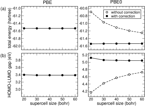
Figure 3: (a) Total energies and (b) energy eigenvalue gaps of naphthalene calculated using the PBE (left panels) and PBE0 (right panels) functionals vs supercell size. To allow a fair comparison, the same energy scales are used in the left and right panels. For PBE0, closed and open symbols indicate values obtained with the singularity correction turned on and off, respectively.

In this section, we present calculations for total energies and energy eigenvalues of small organic molecules. For these calculations, we used the electronic structure scheme based on plane waves and pseudopotentials with large supercells of varying size and $\Gamma$-point sampling. We considered the molecules of naphthalene (C₁₀H₈) and pyridine (C₅H₅N), which are sufficiently small to allow us to investigate the asymptotic behavior for large simulation cells. Furthermore, the eigenvalue of the lowest unoccupied molecular orbital (LUMO) of these molecules is found below the vacuum level, both in PBE and PBE0. In Fig. 3, the total energies and the energy eigenvalue gaps of naphthalene calculated in PBE and PBE0 are plotted as a function of the size of the cubic simulation cell. In hybrid functional calculations, we explicitly compare results obtained with and without the singularity correction $\beta$, i.e. obtained by turning on and off the $\mathbf{G}=0$ component of the exact exchange potential. One notices that both the total energies and the energy eigenvalue gaps calculated in PBE0 show a convergence behavior similar to that achieved in PBE provided the singularity is accounted for. Note that for the largest considered supercell (side of 60 bohr) the singularity correction $\beta$ is still quite sizable and amounts to about 0.2 eV. A similar behavior is observed for pyridine (not shown). These results therefore indicate that in the case of isolated molecular systems, the singularity correction is crucial to achieve well-converged values of total energies and energy eigenvalues in hybrid functional calculations based on plane-wave basis sets.

Table 1: Energy eigenvalues of the highest occupied molecular orbitals ($\varepsilon_{\text{HOMO}}$) and of the lowest unoccupied molecular orbitals ($\varepsilon_{\text{LUMO}}$), energy eigenvalue band gaps ($E_{\text{g}}$), and ionization potentials (IP) of naphthalene and pyridine calculated with the PBE0 functional through a plane-wave (CPMD, Ref. CPMD, ) and an all-electron scheme (Gaussian03, Ref. Gaussian03, ). The eigenvalues are referred to the vacuum level.

		CPMD	Gaussian03
naphthalene	$\varepsilon_{\text{HOMO}}$	$-$6.34	$-$6.28
	$\varepsilon_{\text{LUMO}}$	$-$1.29	$-$1.20
	$E_{\text{g}}$	5.05	5.08
	IP	7.96	7.94
pyridine	$\varepsilon_{\text{HOMO}}$	$-$7.51	$-$7.43
	$\varepsilon_{\text{LUMO}}$	$-$0.98	$-$0.83
	$E_{\text{g}}$	6.53	6.60
	IP	9.51	9.46

To benchmark our hybrid-functional results, we also used an all-electron electronic-structure scheme based on localized atomic orbitals and open boundary conditions.Gaussian03 Total energies cannot be compared because of the different number of electrons that are treated explicitly. The energy eigenvalues and energy gaps are compared with those obtained with the plane-wave scheme in Table 1. The eigenvalues are referred to the vacuum level corresponding to local potential far from the molecule. The agreement between the two sets of calculations is very good. This agreement further supports the validity of the singularity correction derived in Sec. II. To the extent that basis set errors for these molecules are small, the differences also provide an estimate of the way the different treatments of core electrons affect the energy eigenvalues obtained with hybrid functionals. Table 1 also contains calculated ionization potentials, of which the discussion is deferred to Sec. V.1.

IV.2 Extended systems

In this section, we study the effect of the singularity correction in hybrid functional calculations on the total energies and energy eigenvalues of bulk systems. In particular, our purpose is (i) to illustrate the convergence of small-cell calculations with $k$-point sampling (cf. Refs. Carrier_PRB_2007, ; Spencer_PRB_2008, ) and (ii) to study the convergence of $\Gamma$-point calculations with supercell size. In the latter case, one issue of interest is whether the achieved level of convergence is similar to that of corresponding calculations with semilocal functionals.

We chose silicon and $\alpha$-quartz SiO₂ to examine systems with different band gaps. To allow a comparison between PBE and PBE0 calculations of the electronic structure, we used the lattice parameters optimized in the PBE also in the hybrid functional calculations.

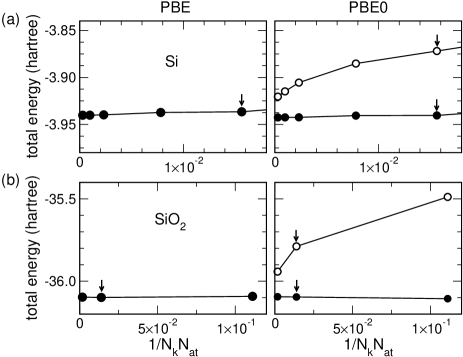
Figure 4: Total energies of (a) Si and (b) $\alpha$-quartz SiO₂ per formula unit versus 1/$N_{k}N_{\text{at}}$, where $N_{k}$ is the total number of $k$-points and $N_{\text{at}}$ the total number of atoms in the supercell. Results obtained in the PBE and the PBE0 are reported in left and right panels, respectively. For PBE0, closed and open symbols indicate values obtained with the singularity correction turned on and off, respectively. Arrows show data points which were also obtained with $\Gamma$-point sampling.

We first considered the convergence of total energies. PBE and PBE0 results for silicon and $\alpha$-quartz are displayed in Fig. 4. The data points illustrate how convergence is achieved with increasing density of $k$-point sampling. For both systems, the inclusion of the singularity correction in the hybrid functional calculations leads to a faster convergence, very similar to that achieved by the semilocal functional. It is apparent that the singularity correction is sizable and that its inclusion significantly speeds up the convergence. For comparison, we also calculated total energies employing large supercells and $\Gamma$-point sampling. In the respective limits of dense $k$-point samplings and large supercell size, the two kinds of calculations give the same converged energies. When the energies calculated in the latter scheme are reported in Fig. 4 (see arrows), they are found to correspond to energies obtained with primitive cells and dense $k$-point samplings. In particular, for finite supercell size, the degree of convergence achieved with hybrid functionals when the singularity is treated is comparable to that obtained with semilocal functionals. These results highlight the importance of including the singularity correction when using hybrid functionals with $\Gamma$-point sampling. This is particularly important when total energies obtained with supercells of different size are comparatively evaluated, such as in the optimization of lattice parameters or in constant-pressure molecular dynamics simulations.

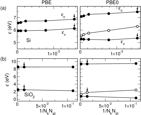
Figure 5: Eigenvalues corresponding to the valence ($\varepsilon_{\rm v}$) and conduction ($\varepsilon_{\rm c}$) band edges of (a) Si and (b) $\alpha$-quartz SiO₂ vs 1/($N_{k}$$N_{\text{at}}$), where $N_{k}$ is the total number of $k$-points and $N_{\text{at}}$ the total number of atoms in the supercell. Results obtained in the PBE and the PBE0 are reported in left and right panels, respectively. For PBE0, closed and open symbols indicate values obtained with the singularity correction turned on and off, respectively. Arrows show data points which were also obtained with $\Gamma$-point sampling. The energies obtained with the two functionals are aligned through the local electrostatic potential (cf. Ref. Alkauskas_PRL_2008, ).

Next, we addressed the convergence of energy band edges and band gaps. The band gap is obtained from the energy eigenvalues:

$$E_{\text{g}}=\varepsilon_{\text{c}}-\varepsilon_{\text{v}}$$ (32)

where $\varepsilon_{\text{c}}$ and $\varepsilon_{\text{v}}$ are the conduction band minimum and the valence band maximum, respectively. In Fig. 5, we give the band gaps of silicon and SiO₂ as a function of $k$-point sampling or supercell size, as obtained within both the PBE and the PBE0. The results obtained with the hybrid functional are given with and without the singularity correction. In analogy with the convergence of the total energy (Fig. 4), the convergence of the band gap is very slow when omitting this correction. The improvement is more clear for SiO₂, for which the band gap converges at a sparser $k$-point density. Results obtained with large supercells and $\Gamma$-point sampling coincide with those obtained with small unit cells and dense $k$-point meshes. We note that in the case of SiO₂ a converged value of the PBE0 band gap is already achieved with a simulation cell of 72 atoms, well within current computationally accessible limits. In the case of Si, the convergence is slower because of the smaller band gap, but the convergence of the hybrid functional result is similar to that achieved with the semilocal functional when the singularity correction is included. In Fig. 5, the convergence of the respective band edges is shown. The singularity correction only affects the occupied states by introducing a constant downward shift of the energies (cf. Sec. II).

Figure 6: Silicon band gap calculated with the PBE (left panel) and PBE0 (right panel) functionals for a cubic simulation cell containing 8 atoms vs number of $k$-points in the [001] direction, $N_{kz}$, with fixed $k$-point sampling in the orthogonal directions ($N_{kx}$=$N_{ky}$=2). For PBE0, closed and open symbols indicate values obtained with the singularity correction turned on and off, respectively.

In many applications concerning surfaces and interfaces, the supercells have an elongated shape to describe the transition across the boundary region. For such systems, the omission of the singularity correction in a hybrid functional calculation in which a $\Gamma$-point sampling is used leads to a peculiar behavior of total energies and single particle eigenvalues. To simulate these conditions, we considered a cubic 8-atom simulation for bulk silicon and increased the $k$-point sampling along the [001] direction, while keeping the $k$-point sampling in the orthogonal directions constant. This description is equivalent to that achieved with an elongated supercell calculation in which the Brillouin zone is sampled at the sole $\Gamma$ point. Figure 6 shows the calculated band gap vs. the number of $k$-points in the [001] direction. Omitting the singularity correction leads in this case to a linear increase of the band gap. A similar linear increase is also found for the total energy (not shown). In neither case, it is therefore possible to obtain a converged value. Including the singularity correction reestablishes a converging behavior that resembles that found in semilocal density functional calculations.

From the result in Fig. 6, we infer that the singularity corrections for elongated simulation cells may change sign in comparison with cubic unit cells and/or isotropic $k$-point meshes. To understand this behavior, it is useful to recall that, in the case of $\Gamma$-point sampling, the singularity correction is proportional to the energy per unit cell of a periodically repeated point charge immersed in a compensating background. In case of nearly cubic supercells the latter energy is negative, i.e. the attractive interaction of the point charge with the uniform background is larger than the repulsive interactions between the point charge and its images. When the shape of the cell elongates in one or two directions, the repulsive interaction with the image charges in the orthogonal directions grows because of the reduced screening. For sufficiently elongated shapes, this repulsive interaction dominates and the sign of the point-charge energy switches.

To summarize the results of this section, we showed that the singularity correction is needed to obtain converged total energies and single-electron eigenvalues in hybrid functional calculations with small unit cell and dense $k$-point samplings, in accord with previous studies.Carrier_PRB_2007 ; Spencer_PRB_2008 Furthermore, we showed that hybrid functional calculations with large supercells and $\Gamma$-point samplings also benefit from the singularity correction, yielding levels of convergence which are similar to those achieved with semilocal functionals. In the case of $\Gamma$-point samplings, the singularity correction applies to both molecular and extended systems in a qualitatively similar way.

V Charged systems: Localized states

In the following, we discuss convergence issues associated to charged systems when using hybrid functional schemes based on plane wave basis sets. Charged systems occur in several circumstances, such as, for example, when studying charged molecules, defects, ions in liquids, etc. We here focus on the determination of total energy differences between different charge states and the way the singularity correction affects the convergence properties. We are particularly interested in assessing how the convergence properties of hybrid functional calculations compare with those of semilocal density functional calculations. For simplicity, we consider from now on only systems in which the electronic structure is sampled through the sole $\Gamma$ point. The convergence is therefore studied with respect to increasing simulation cell, or equivalently with respect to decreasing singularity correction. Generalization to convergence with $k$-point samplings is trivial. In this section, we deal with atomically localized states, either in finite systems or as defect states in solids. Infinitely delocalized states are discussed in Sec. VI. In this work, we do not consider states showing intermediate degrees of localization. For a discussion of the latter, we defer the reader to Refs. Ogut_PRL_1998, .

V.1 Finite systems

To illustrate the convergence of total energy differences between different charge states, we considered the calculation of the ionization potential (IP) of an isolated molecule:

$$\text{IP}=E_{N-1}-E_{N},$$ (33)

where $E_{N}$ is the total energy of the neutral molecule and $E_{N-1}$ the total energy of the same molecule in which one electron has been removed. The total energy calculations correspond to an isolated molecule placed in a large supercell and subject to periodic boundary conditions. This technical constraint introduces a spurious interaction between the localized charge and the neutralizing background charge, which needs to be considered in order to speed up the convergence.Makov_PRB_1995 This correction depends on the size of the simulation cell, but applies indifferently to both hybrid functionals and semilocal density functionals. In our calculations, the dominant correction corresponding to the charge monopole has systematically been included.Makov_PRB_1995

Figure 7: Ionization potential (IP) of naphthalene calculated with the PBE (left panel) and PBE0 (right panel) functionals for cubic simulation cells vs singularity correction $\beta$, which scales like the inverse of the simulation cell size. For PBE0, closed and open symbols indicate values obtained with the singularity correction turned on and off, respectively.

In Fig. 7, we give the ionization potentials of naphthalene calculated within both the PBE and the PBE0 for different supercell sizes. The PBE0 results are obtained by both including and dismissing the singularity correction. The results are plotted as a function of the singularity correction, which scales like the inverse of the simulation cell size. For the simulation cells considered (cubic cells with sides ranging between 20 and 60 bohr), the PBE results are already close to the converged values obtained by linear extrapolation. The same consideration applies for the PBE0 results which include the singularity correction. However, in absence of singularity correction, the error with respect to the converged values is significantly larger. The converged PBE0 values for the ionization potentials of naphthalene and pyridine are reported in Table 1, where they are compared with results obtained with an all-electron scheme based on localized orbitals. The values calculated within the two schemes differ by less than 0.05 eV.

It is of interest to extend our comparative study between PBE and PBE0 calculations to the approximate scheme based on Slater’s transition state.Slater_AQC_1972 According to the integral form of Janak’s theorem,Janak_PRB_1978 the total-energy difference of Eq. (33) is given by

$$E_{N-1}-E_{N}=-\int_{0}^{1}\varepsilon_{n}(f)df,$$ (34)

where $\varepsilon_{n}(f)$ describes the eigenvalue of the highest occupied eigenstate $n$ as it varies with its fractional occupation $f$. Using the trapezoidal rule for the integral, we obtain Slater’s approximation:

$$E_{N-1}-E_{N}\approx-\varepsilon_{n}({1}/{2})\approx-\left[\varepsilon_{n}(0)+\varepsilon_{n}(1)\right]/2,$$ (35)

where we further approximated the eigenvalue at half-filling by an average at integer occupations. For the molecules investigated here, this approximation is found to give accurate results for both the semilocal and the hybrid functional (not shown). Note that, in the latter case, the singularity corrections of energies and eigenvalues are compatible with the relation in Eq. (35). Indeed, this approximation equally holds for corrected energies and eigenvalues as for uncorrected ones. Similar considerations apply to electron removal energies.

V.2 Defects in solids

The discussion pertaining to total energy differences of finite systems (Sec. V.1) applies with minor modifications to the study of localized defect states in solids. In this case, the relevant physical quantities, the charge transition levels, are also expressed as total energy differences. Defect formation energies are first determined for varying electron chemical potential $\mu$:VanDeWalle_JAP_2004

$$E_{\text{f}}^{q}(\mu)=E^{q}_{\text{tot}}-E^{\text{bulk}}_{\text{tot}}-\sum_{\alpha}n_{\alpha}\eta_{\alpha}+q(\mu+\varepsilon_{\text{v}}+\Delta V)+E_{\text{corr}}^{q},$$ (36)

where $E^{q}_{\text{tot}}$ is the total energy of the defect system carrying a charge $q$, $E^{\text{bulk}}_{\text{tot}}$ the total energy of the unperturbed system, $n_{\alpha}$ the number of extra atoms of species $\alpha$ needed to create the defect, and $\eta_{\alpha}$ the corresponding atomic chemical potential. The chemical potential $\mu$ is referred to the valence band maximum $\varepsilon_{\text{v}}$. $\Delta V$ is a correction which is applied in order to align the local potential far away from the neutral defect to that of the unperturbed bulk.VanDeWalle_JAP_2004 The correction $E_{\text{corr}}^{q}$ describes the spurious interaction of the added charge with the compensating background charge.Makov_PRB_1995 As commented in Sec. II.1, the leading term of this correction pertaining to the monopole can be expressed as

$$E_{\text{corr}}^{q}=\frac{q^{2}\chi}{2\epsilon},$$ (37)

where $\chi$ is defined in Eq. (12) and $\epsilon$ is the dielectric constant of the unperturbed bulk system. In our calculations, this correction is applied systematically in both PBE and PBE0 calculations.

Charge transition levels correspond to specific values of the electron chemical potential for which two charge states have equal formation energies. For example, the charge transition level $\mu_{q/q^{\prime}}$ between two charge states $q$ and $q^{\prime}$ is defined by the condition $E_{\text{f}}^{q}=E_{\text{f}}^{q^{\prime}}$ and is thus given by the following expression:

$$\mu_{q/q^{\prime}}=\frac{\left(E_{\text{\text{f}}}^{q^{\prime}}-E_{\text{\text{f}}}^{q}\right)+\left(E_{\text{corr}}^{q^{\prime}}-E_{\text{corr}}^{q}\right)}{q-q^{\prime}}-(\varepsilon_{\text{v}}+\Delta V).$$ (38)

In this expression the dependence on the atomic chemical potentials $\eta$ drops out and the defect charge transition level is basically determined by a total energy difference between different charge states of the defect. In this sense, these quantities are counterparts of the ionization potentials and electron affinities of isolated atomic and molecular systems. The charge transition levels of localized defect states can also be obtained in a very accurate way through the energy eigenvalues by the application of Janak’s theorem both in PBE and in PBE0 [Eq. (35)].Alkauskas_PhB_2007b

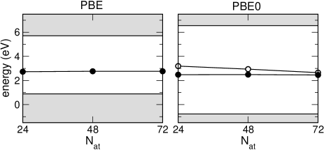
Figure 8: Vertical charge transition levels $\mu_{+/0}$ associated to the hydrogen bridge defect in $\beta$-crystobalite as obtained with the PBE (left panel) and the PBE0 (right panel) functionals vs number of atoms $N_{\text{at}}$ in the simulation cell. For PBE0, closed and open symbols indicate values obtained with the singularity correction turned on and off, respectively. The indicated valence and conduction band edges correspond to the converged energy eigenvalues. The energies obtained with the two functionals are aligned through the local electrostatic potential (cf. Ref. Alkauskas_PRL_2008, ).

We illustrate the convergence behavior of charge transition levels for the hydrogen bridge defect (hydrogen substitutional to oxygen) in $\beta$-crystobalite SiO₂. In particular, we focused on the vertical charge transition level $\mu_{+/0}$ located at approximately mid gap.Bloechl_PRB_2000 ; Alkauskas_PhB_2007 We considered three different supercells in which one lateral size was varied while the other dimensions were kept fixed, i.e. we used 2$\times$2$\times$2, 2$\times$2$\times$3, and 2$\times$2$\times$4 unit cells. Such elongated cells might for instance occur when slab models are adopted. Charge transition levels calculated in the PBE and in the PBE0 are shown in Fig. 8 for increasing number of atoms in the simulation cell. The results obtained with the two functionals are aligned through the local electrostatic potential, as suggested by the study in Ref. Alkauskas_PRL_2008, . It clearly appears that the PBE and PBE0 defect levels show a similar convergence behavior, provided the singularity correction is included in the PBE0 calculation. The singularity correction is crucial to achieve this level of convergence. Without the singularity correction, the charge transition levels are clearly not converged for the range of simulation cells considered. It is clearly seen that the convergence behavior of charge transition levels of defects is analogous to that of energy transitions in finite systems (Sec. V.1).

VI Charged systems: Delocalized states

The case in which the extra charge is carried by extended delocalized states requires special attention. Let us assume an infinite solid with a energy eigenvalue spectrum $\varepsilon_{k}$. The energy cost of adding one electron to the previously unoccupied state $n$ is simply given by

$$E_{N+1}-E_{N}=\varepsilon_{n},$$ (39)

where we used Janak’s theoremJanak_PRB_1978 as formulated in Eq. (34) and the fact that energy eigenvalues in infinite solids do not depend on the occupation of the state. Identical considerations also apply for electron removal energies. On this basis, it is possible to express the valence and conduction band edges in terms of total energy differences between systems of different charge:

$$\tilde{\varepsilon}_{\text{c}} = E_{N+1}-E_{N},$$ (40)

$$\tilde{\varepsilon}_{\text{v}} = E_{N}-E_{N-1}.$$ (41)

Consequently, the energy band gap can also be obtained as

$$\tilde{E}_{\text{g}}=\tilde{\varepsilon}_{\text{c}}-\tilde{\varepsilon}_{\text{v}}=E_{N+1}+E_{N-1}-2E_{N}.$$ (42)

In our notation, the tilde sign signifies that the concerned quantity is obtained from a total energy difference, as opposed to a direct derivation from the spectrum of energy eigenvalues.

In practical calculations, the supercells always have finite size, by which the band edges determined by total-energy difference differ from the actual energy eigenvalues:Lany_PRB_2008

$$\tilde{\varepsilon}_{\text{c}} = {\varepsilon}_{\text{c}}+\Delta\varepsilon_{\text{c}},$$ (43)

$$\tilde{\varepsilon}_{\text{v}} = {\varepsilon}_{\text{v}}+\Delta\varepsilon_{\text{v}},$$ (44)

where it is understood that

$$\lim_{\Omega\rightarrow\infty}\Delta\varepsilon_{\text{c}} = 0,$$ (45)

$$\lim_{\Omega\rightarrow\infty}\Delta\varepsilon_{\text{v}} = 0,$$ (46)

where $\Omega$ is the volume of the simulation cell. Similarly, we define

$$\tilde{E}_{\text{g}}={E}_{\text{g}}+\Delta E_{\text{g}},$$ (47)

where $\Delta E_{\text{g}}=\Delta\varepsilon_{\text{c}}-\Delta\varepsilon_{\text{v}}$.

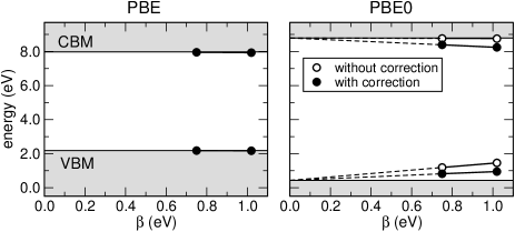
Figure 9: Band edges of $\alpha$-quartz calculated with the PBE (left) and PBE0 (right) functionals as total energy differences vs singularity correction $\beta$ that characterizes the simulation cell, the limit of infinite simulation cell being achieved for vanishing $\beta$. For PBE0, closed and open symbols indicate values obtained with the singularity correction turned on and off, respectively. The energies obtained with the functionals are aligned as in Fig. 5.

We first focus on results obtained with the semilocal density functional. For illustration, we considered $\alpha$-quartz SiO₂ and used simulation cells of varying size. In Fig. 9, we report the band edges calculated using the total energy differences given in Eqs. (40) and (41), and compare them with the converged energy eigenvalues. For the simulation cells considered here, the band edges obtained in the two different ways are essentially identical, i.e. $\Delta\varepsilon_{\text{c}}\approx 0$ and $\Delta\varepsilon_{\text{v}}\approx 0$.

Figure 9 also shows corresponding results obtained with hybrid functionals. In contrast to the behavior found for semilocal functionals, we now encounter a much slower convergence. In other words, in hybrid functional calculations, $\Delta\varepsilon_{\text{c}}$ and $\Delta\varepsilon_{\text{v}}$ are significantly larger than in semilocal density functional calculations performed with the same simulation cells. Therefore, we infer that this behavior should be ascribed to the singular behavior of the exchange interaction.

Figure 10: Difference between band edges of $\alpha$-quartz evaluated through total energy differences ($\tilde{\varepsilon}_{\rm c}$, $\tilde{\varepsilon}_{\rm v}$) and as energy eigenvalues (${\varepsilon}_{\rm c}$, ${\varepsilon}_{\rm v}$) in the PBE (left panel), (b) in the PBE0 with singularity turned off (middle panel), and (c) in the PBE0 with the singularity correction turned on (right panel). The results are plotted against the singularity correction $\beta$. In the right panel, the dashed lines correspond to $\Delta\varepsilon_{\rm c}=-\beta/2$ and $\Delta\varepsilon_{\rm v}=+\beta/2$.

In order to understand this behavior, we reason as follows. The relations given by Eqs. (43) and (44) follow from the Janak theorem and apply to any analytical functional. Therefore, they also apply to a case functional which is specific to a given simulation cell and a given basis set. We further define the case functional by setting the $\mathbf{G}=0$ component of the exchange potential to zero, which corresponds to the label “uncorr” introduced earlier. For this case functional, $\Delta\varepsilon_{\text{c}}$ and $\Delta\varepsilon_{\text{v}}$ are expected to behave in a similar way as for a semilocal functional. Hence, for simulation cells large enough to yield vanishing $\Delta\varepsilon_{\text{c}}$ and $\Delta\varepsilon_{\text{v}}$ with the semilocal functional, we similarly expect vanishing $\Delta\varepsilon^{\text{uncorr}}_{\text{c}}$ and $\Delta\varepsilon^{\text{uncorr}}_{\text{v}}$. This implies

$$\varepsilon^{\text{uncorr}}_{\text{c}} \approx E^{\text{uncorr}}_{N+1}-E^{\text{uncorr}}_{N},$$ (48)

$$\varepsilon^{\text{uncorr}}_{\text{v}} \approx E^{\text{uncorr}}_{N}-E^{\text{uncorr}}_{N-1}.$$ (49)

As shown in the first two panels in Fig. 10, this behavior is numerically confirmed for our case study of $\alpha$-quartz.

Using the relationship between corrected and uncorrected quantities determined in Eqs. (17) and (20), we then derive:

$$\varepsilon^{\text{corr}}_{\text{c}} \approx E^{\text{corr}}_{N+1}-E^{\text{corr}}_{N}+\beta/2,$$ (50)

$$\varepsilon^{\text{corr}}_{\text{v}} \approx E^{\text{corr}}_{N}-E^{\text{corr}}_{N-1}-\beta/2.$$ (51)

In other words, hybrid functional calculations in finite simulation cells give

$$\Delta\varepsilon_{\text{c}} \approx -\beta/2,$$ (52)

$$\Delta\varepsilon_{\text{v}} \approx +\beta/2.$$ (53)

This result is graphically illustrated for $\alpha$-quartz in the third-column panels of Fig. 10. For the band gap, this implies:

$$\Delta E_{\text{g}}\approx-\beta.$$ (54)

We note that the remaining dependence of both $\tilde{\varepsilon}_{\text{c}}$ and $\tilde{\varepsilon}_{\text{v}}$ on $\beta$ does not result from the integration of the singularity, since the results in the third panel in Fig. 10 already refer to “corrected” results. The remaining differences rather originate from the exchange selfinteraction associated to the extra charge, which vanishes slowly with increasing simulation cell. Hence, this behavior is not specific to the use of plane-wave basis sets and should also manifest in implementations based on other basis functions.

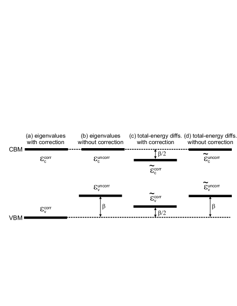
Figure 11: Schematic representation of the band edges determined with hybrid functionals in the presence of a limited $k$ point sampling: as energy eigenvalues (a) with and (b) without accounting for the singularity correction and through total energy differences (c) with and (d) without singularity correction. The result in (a) shows the fastest convergence with simulation cell.

Our findings concerning the energy eigenvalues are schematically illustrated in Fig. 11. The scheme refers to a case in which all quantities would already be converged with simulation cell size, if it were not for the occurrence of exact exchange. Figure 11(a) refers to the corrected energy eigenvalues and corresponds to the converged result. Figure 11(b) shows the eigenvalues in the “uncorrected” case. The singularity correction shifts the occupied states downwards by $\beta$, leaving the unoccupied ones unaffected. Figure 11(c) refers to the determination of band edges through the use of total-energy differences. It is seen that the band edges obtained in this way still differ from the converged levels, despite the use of “corrected” quantities. The valence band edge is overestimated by $\beta/2$, whereas the conduction band edge is underestimated by $\beta/2$. Consequently, the band gap is underestimated by $\beta$ through this approach. Figure 11(d) also refers to band edges obtained through total energy differences but without including the singularity correction. One obtains the same result as in Fig. 11(b), illustrating thereby that the integration of the singularity in the exchange term is responsible for the slow convergence of the band edges calculated by total-energy differences.

VII Conclusions

In this work, we investigated the use of hybrid functionals in plane-wave implementations, in comparison with semilocal density functionals. The main objective consisted in determining whether a hybrid functional calculation requires a $k$-point sampling of increased density in order to properly integrate the singularity appearing in the exact nonlocal exchange energy. This issue is of particular importance when dealing with large simulation cells, where an excessive increase of the $k$-point sampling would make the calculation computationally prohibitive. Typical applications include surface, interface, and defect calculations, but also molecular dynamics simulations.

To treat the divergence, we adopted a formulation which consists in transforming the integrand into a regular function through the use of an auxiliary function that can be integrated analytically.Gygi_PRB_1986 Through the use of an appropriate auxiliary function,Massidda_PRB_1993 this formulation can trivially be extended to calculations with large simulation cells and low-density $k$-point samplings. In the case of $\Gamma$-point sampling, the sampling of reciprocal space is achieved through the reciprocal lattice vectors, which densify as the simulation cell grows. We further used a formulation which recasts the treatment of the divergence in the form of singularity correction terms.Carrier_PRB_2007 These terms intervene in the total energy and in the energy eigenvalues of the occupied states.

In the present investigation, we found it convenient to distinguish finite and extended systems, localized and delocalized states, and neutral and charged calculations. The general conclusion is that the same $k$-point samplings used in semilocal density functional calculations yield a comparable level of convergence in hybrid functional calculations, provided the singularity corrections are accounted for. However, our study highlights a few points that deserve special attention.

The first point concerns the treatment of screened exchange. While screened exchange does not show any singularity, it is nevertheless recommended to adopt the proposed scheme also in this case in order to achieve the same convergence properties as achieved with semilocal density functionals.

The second noteworthy point concerns applications in which the sampling in reciprocal space around the divergence is anisotropic. This is for instance the case for calculations with elongated simulation cells and $\Gamma$-point samplings, as often occurs in the study of surfaces and interfaces. In such cases, the singularity correction terms are critical for achieving not only well converged properties but also a qualitatively correct behavior.

The final point that deserves attention and which is unusual with respect to ordinary semilocal density functional calculations concerns the determination of band edges and band gaps of extended systems through total energy differences. Our study shows that band edges determined in this way converge slower in hybrid functional calculations because of the exchange selfinteraction associated to the extra charge. This convergence problem arises for delocalized states but does not occur for localized states of point defects or of finite molecular systems.

In conclusion, the correct treatment of the singularity can be achieved without requiring any significant computational overhead. This opens the way for using hybrid functionals in very much the same way as ordinary semilocal functionals. To date, the scheme described in this work has already led to several successful applications including studies of amorphous systems,Broqvist_APL_2007 defects,Broqvist_APL_2006 ; Broqvist_APL_2008 ; Alkauskas_PRL_2008 ; Broqvist_PRB_2008 ; Alkauskas_PRB_2008 ; Broqvist_JAP_2009 and interfaces.Devynck_PRB_2007 ; Devynck_APL_2007 ; Broqvist_APL_2008 ; Alkauskas_PRL_2008b ; Devynck_SS_2008 ; Broqvist_APL_2009

References

- (1) P. Hohenberg and W. Kohn, Phys. Rev. 136, B864 (1964).
- (2) W. Kohn and L. J. Sham, Phys. Rev. 140, A1133 (1965).
- (3) J. P. Perdew and Y. Wang, Phys. Rev. B 33, 8800 (1986).
- (4) A. D. Becke, J. Chem. Phys. 84, 4524 (1986).
- (5) A. D. Becke, Phys. Rev. A 38, 3098 (1988).
- (6) J. P. Perdew et al., Phys. Rev. B 46, 6671 (1992).
- (7) J. P. Perdew, K. Burke, and M. Ernzerhof, Phys. Rev. Lett. 77, 3865 (1996).
- (8) A. D. Becke, J. Chem. Phys. 98, 1372 (1993).
- (9) A. D. Becke, J. Chem. Phys. 98, 5648 (1993).
- (10) L. A. Curtiss, K. Raghavachari, P. C. Redfern, and J. A. Pople, J. Chem. Phys. 106, 1063 (1997).
- (11) L. A. Curtiss, P. C. Redfern, K. Raghavachari, and J. A. Pople, J. Chem. Phys. 109, 42 (1998).
- (12) J. Heyd and G. E. Scuseria, J. Chem. Phys. 121, 1187 (2004); J. Heyd, J. E. Peralta, G. E. Scuseria, and R. L. Martin, J. Chem. Phys. 123, 174101 (2005).
- (13) J. Paier, M. Marsman, K. Hummer, G. Kresse, I. C. Gerber, and J. G. Ángáyan, J. Chem. Phys. 124, 154709 (2006); 125, 249901 (E) (2006).
- (14) J. Muscat, A. Wander, and N. M. Harrison, Chem. Phys. Lett. 342, 397 (2001).
- (15) B. G. Janesko, T. M. Henderson, and G. E. Scuseria, Phys. Chem. Chem. Phys. 11, 443 (2009).
- (16) J. Paier, R. Hirschl, M. Marsman, and G. Kresse, J. Chem. Phys. 122, 234102 (2005).
- (17) C. Di Valentin, G. Pacchioni, and A. Selloni, Phys. Rev. Lett. 97, 166803 (2006).
- (18) C. G. Van de Walle and J. Neugebauer, J. Appl. Phys. 95, 3851 (2004).
- (19) G. Pacchioni, F. Frigoli, D. Ricci, and J. A. Weil, Phys. Rev. B 63, 054102 (2000).
- (20) S. B. Zhang, S.-H. Wei, and A. Zunger, Phys. Rev. B, 63, 075205 (2001).
- (21) J. M. Knaup, P. Deák, T. Frauenheim, A. Gali, Z. Hajnal, and W. J. Choyke, Phys. Rev. B 72, 115323 (2005).
- (22) P. Deák, A. Gali, A. Sólyom, A. Buruzs, and T. Frauenheim, J. Phys. Cond. Mat. 17, S2141 (2005).
- (23) K. Xiong, J. Robertson, M. C. Gibson, and S. J. Clark, Appl. Phys. Lett. 87, 183505 (2005).
- (24) J. L. Gavartin, D. Muñoz Ramo, A. L. Shluger, G. Bersuker, and B. H. Lee, Appl. Phys. Lett. 89, 082908 (2006).
- (25) P. Broqvist and A. Pasquarello, Appl. Phys. Lett. 89, 262904 (2006).
- (26) S. Lany and A. Zunger, Phys. Rev. Lett. 98, 045501 (2007).
- (27) A. Janotti and C. G. Van de Walle, Phys. Rev. B 76, 165202 (2007).
- (28) P. Broqvist, A. Alkauskas, and A. Pasquarello, Appl. Phys. Lett. 92, 132911 (2008).
- (29) A. Alkauskas, P. Broqvist, and A. Pasquarello, Phys. Rev. Lett. 101, 046405, (2008).
- (30) P. Broqvist, A. Alkauskas, and A. Pasquarello, Phys. Rev. B 78, 075203 (2008).
- (31) T. R. Paudel and W. R. L. Lambrecht, Phys. Rev. B 77, 205202 (2008).
- (32) F. Oba, A. Togo, I. Tanaka, J. Paier, and G. Kresse, Phys. Rev. B 77, 245202 (2008).
- (33) A. Alkauskas, P. Broqvist, and A. Pasquarello, Phys. Rev. B 78, 161305(R) (2008).
- (34) S. Lany and A. Zunger, Phys. Rev. B 78, 235104 (2008).
- (35) C. Pisani and R. Dovesi, Int. J. Quantum Chem. 17, 501 (1980); R. Dovesi, R. Orlando, C. Roetti, C. Pisani, and V. R. Saunders, Phys. Stat. Sol. 217, 63 (2000).
- (36) Gaussian 03, Revision C.02, M. J. Frisch et al., Gaussian, Inc., Wallingford CT, 2004.
- (37) M. C. Payne, M. P. Teter, D. C. Allan, T. A. Arias, and J. D. Joannopoulos, Rev. Mod. Phys. 64, 1045 (1992).
- (38) S. Chawla and G. A. Voth, J. Chem. Phys. 108, 4697 (1998).
- (39) A. Sorouri, W. M. C. Foulkes, and N. D. M. Hine, J. Chem. Phys. 124, 064105 (2006).
- (40) T. Todorova, A. P. Seitsonen, J. Hutter, I.-F. W. Kuo, and C. J. Mundy, J. Phys. Chem. B 110, 3685 (2006).
- (41) R. Car and M. Parrinello, Phys. Rev. Lett. 55, 2471 (1985); J. Hutter and A. Curioni, ChemPhysChem 6, 1788 (2005); CPMD, Copyright IBM Corp 1990-2006, Copyright MPI für Festkörperforschung Stuttgart 1997-2001.
- (42) A. Alkauskas, P. Broqvist, F. Devynck, and A. Pasquarello, Phys. Rev. Lett. 101, 106802 (2008).
- (43) C. Kittel, Quantum Theory of Solids (John Wiley & Sons, New York, 1963).
- (44) F. Gygi and A. Baldereschi, Phys. Rev. B 34, 4405 (1986).
- (45) S. Massidda, M. Posternak, and A. Baldereschi, Phys. Rev. B 48, 5058 (1993).
- (46) P. Carrier, S. Rohra, and A. Görling, Phys. Rev. B 75, 205126 (2007).
- (47) H.-V. Nguyen and S. de Gironcoli, Phys. Rev. B 79, 205114 (2009).
- (48) J. Spencer and A. Alavi, Phys. Rev. B 77, 193110 (2008).
- (49) X. Wu, A. Selloni, and R. Car, Phys. Rev. B 79, 085102 (2009).
- (50) Y. Wang, S. de Gironcoli, N. S. Hush, and J. R. Reimers, J. Am. Chem. Soc. 129, 10402 (2007).
- (51) A. Stroppa and G. Kresse, New J. Phys. 10, 063020 (2008).
- (52) S. Kümmel and L. Kronik, Rev. Mod. Phys. 80, 3 (2008).
- (53) M. Städele, M. Moukara, J.A. Majewski, P. Vogl, and A. Görling, Phys. Rev. B 59, 10031 (1999).
- (54) P. P. Ewald, Ann. Phys. (Leipzig) 64, 253 (1921).
- (55) J. Heyd, G. E. Scuseria, and M. Enzerhof, J. Chem. Phys. 118, 8207 (2003); ibid 124, 219906 (E) (2006).
- (56) A. V. Krukau, O. A. Vydrov, A. F. Izmaylov, and G. E. Scuseria, J. Chem. Phys. 125, 224106 (2006).
- (57) J. P. Perdew, K. Burke and M. Ernzerhof, J. Chem. Phys. 105, 9982 (1996).
- (58) N. Troullier and J. L. Martins, Phys. Rev. B 43, 1993 (1991).
- (59) S. Goedecker, M. Teter, and J. Hutter, Phys. Rev. B 54 (1996) 1703.
-
(60)
P. Giannozzi et al., unpublished (2009);
http://www.quantum-espresso.org/ - (61) S. Öǧüt, J. R. Chelikowsky, and S. G. Louie, Phys. Rev. Lett. 80, 3162 (1998); R. W. Godby and I. D. White, ibid. 80, 3161 (1998).
- (62) G. Makov and M. C. Payne, Phys. Rev. B 51, 4014 (1995).
- (63) J. C. Slater, Adv. Quantum Chem. 6, 1 (1972).
- (64) J. F. Janak, Phys. Rev. B 18, 7165 (1978).
- (65) A. Alkauskas and A. Pasquarello, Physica B 401-402, 670 (2007).
- (66) P. E. Blöchl, Phys. Rev. B 62, 6158 (2000).
- (67) A. Alkauskas and A. Pasquarello, Physica B 401-402, 546 (2007).
- (68) P. Broqvist and A. Pasquarello, Appl. Phys. Lett. 90, 082907 (2007).
- (69) P. Broqvist, A. Alkauskas, J. Godet, and A. Pasquarello, J. Appl. Phys. 105, 061603 (2009).
- (70) F. Devynck, F. Giustino, P. Broqvist, and A. Pasquarello, Phys. Rev. B 76, 075351 (2007).
- (71) F. Devynck, Ž. Šljivančanin, and A. Pasquarello, Appl. Phys. Lett. 91, 061930 (2007).
- (72) F. Devynck and A. Pasquarello, Surf. Sci. 602, 2989 (2008).
- (73) P. Broqvist, J. F. Binder, and A. Pasquarello, Appl. Phys. Lett. 94, 141911 (2009).