Sulfur Abundances in the Orion Association B Stars

Abstract

Sulfur abundances are derived for a sample of ten B main-sequence star members of the Orion association. The analysis is based on LTE plane-parallel model atmospheres and non-LTE line formation theory by means of a self-consistent spectrum synthesis analysis of lines from two ionization states of sulfur, S ii and S iii. The observations are high-resolution spectra obtained with the ARCES spectrograph at the Apache Point Observatory. The abundance distribution obtained for the Orion targets is homogeneous within the expected errors in the analysis: A(S)=7.15$\pm$0.05. This average abundance result is in agreement with the recommended solar value (both from modelling of the photospheres in 1-D and 3-D, and meteorites) and indicates that little, if any, chemical evolution of sulfur has taken place in the last $\sim$4.5 billion years. The sulfur abundances of the young stars in Orion are found to agree well with results for the Orion nebulae, and place strong constraints on the amount of sulfur depletion onto grains as being very modest or nonexistent. The sulfur abundances for Orion are consistent with other measurements at a similar galactocentric radius: combined with previous results for other OB-type stars produce a relatively shallow sulfur abundance gradient with a slope of $-0.037\pm$0.012 dex Kpc^-1.

1 Introduction

The chemical element sulfur, together with O, Ne, Mg, Si, Ar and Ca, belongs to the family of the so-called $\alpha$-capture elements, which are light elements with even Z in the range between 6 $<$ Z $<$ 22. Sulfur is among the ten most abundant elements in the universe and its production occurs both during hydrostatic and explosive oxygen-burning phases in massive star evolution and supernovae of Type ii (SN ii; Clayton 2003). Although some contribution from SN ia’s is also expected (François 2004, and references therein).

The observed evolution of the sulfur abundance in the Galaxy is generally less well-defined than that of other $\alpha$-elements (such as oxygen or calcium). The earliest determinations of sulfur abundances in stars dates from 1980’s (Clegg et al., 1981; François, 1987, 1988). More recently, Chen et al. (2002) studied S i lines in a sample of disk stars (with [Fe/H] $>$ -1.0) and found that sulfur abundances correlate with those of silicon, as generally expected since these are both considered to be $\alpha$-elements. Concerning the behavior of [S/Fe] versus [Fe/H] in low-metallicity halo stars, Israelian & Rebolo (2001) and Takada-Hidai et al. (2002) found that [S/Fe] increased linearly with decreasing [Fe/H], while Ryde & Lambert (2004) and Nissen et al. (2004) obtained values of [S/Fe] that are roughly constant and enhanced relative to solar value for metal poor stars, following the general trend observed for other $\alpha$-capture elements. Caffau et al. (2005), on the other hand, found at low metallicities both a population of stars having a flat [S/Fe] $\sim$ +0.4 dex, and stars with higher [S/Fe] ratios. The recent results by Nissen et al. (2007), which take into account corrections for non-LTE effects, indicate that halo stars follow a plateau at [S/Fe] $\sim$ +0.2 dex.

An important property of sulfur, a volatile element, is that given its low condensation temperature it is not expected to locked-up significantly into grains, at least not in the low-density interstellar medium, nor in certain nebular sites (Goicoechea et al., 2006). Thus, a comparison between nebular and stellar sulfur abundances may involve relatively small corrections for grain depletion; if true, sulfur then would provide a direct connection between the stellar and gas-phase abundances in the interstellar medium, as well as nebular abundances in galactic and extra-galactic environments. This work will focus on defining the present-day stellar sulfur abundance in a sample of young B-star members of the Orion association. These abundances can be used to help define the present-day sulfur abundance in the solar neighborhood, as well as constrain sulfur depletions onto grains. In addition, the Orion sample provides another data point to define the Galactic disk sulfur abundance gradient.

2 Observational Data

The targets are 10 main-sequence early B-type star members of the Ori OB1 association, selected from the sample of Cunha & Lambert (1994) and previously analyzed for neon abundances in Cunha et al. (2006). The observational data are high resolution (R$\sim$35,000) spectra obtained with the Astrophysical Research Consortium (ARC) Echelle Spectrograph on the 3.5m telescope at the Apache Point Observatory in 2007. The spectra cover the wavelength range between 3480–10260Å and have signal-to-noise ratios generally greater than $\sim$100. The data were reduced and the spectra were extracted and normalized to a unity continuum following standard procedures. In Figure 1 we show sample spectra for all target stars in the spectral region between 4800Å–4832Å  where the S ii lines at 4815Å and 4824Å are found. More details about the observations and data reduction can be found in Lanz et al. (2008).

3 Stellar Parameters and Sulfur Abundance Determinations

The stellar parameters, effective temperature, surface gravity, and microturbulent velocity, adopted in this analysis are listed in Table 1 and taken from Cunha & Lambert (1994). The values of T_eff and $\log g$ in that study were obtained from an iterative scheme which combines photometric calibrations for the Strömgren indices $c_{o}$, [$c_{1}$], and $\beta$ and fitting of LTE theoretical profiles to the H$\gamma$ line wings. The microturbulence, $\xi$, was derived from an analysis of O ii lines, by requiring that the oxygen abundances are independent of the line strength.

Sulfur abundances for a sample of 16 S ii and 3 S iii lines were derived from non-LTE synthetic profiles and adopting LTE model atmospheres from Kurucz (1993) plus a sulfur model atom from Vrancken et al. (1996). Our line sample was selected from the Kurucz linelist and included all S ii and S iii lines within 4000 – 5100 Å with profiles which could be synthesized (corresponding to a minimum equivalent width $\sim$ 2 mÅ) and which were relatively free of blends. The adopted model atom treats S ii/S iii simultaneously with 81 levels of S ii and 21 levels of S iii and also includes the three lowest levels of S i and the two lowest levels of S iv, together with the ground state of S v. The solutions to the statistical equilibrium and transfer equations were obtained with the program DETAIL (Giddings, 1981) which assumes LS-coupling.

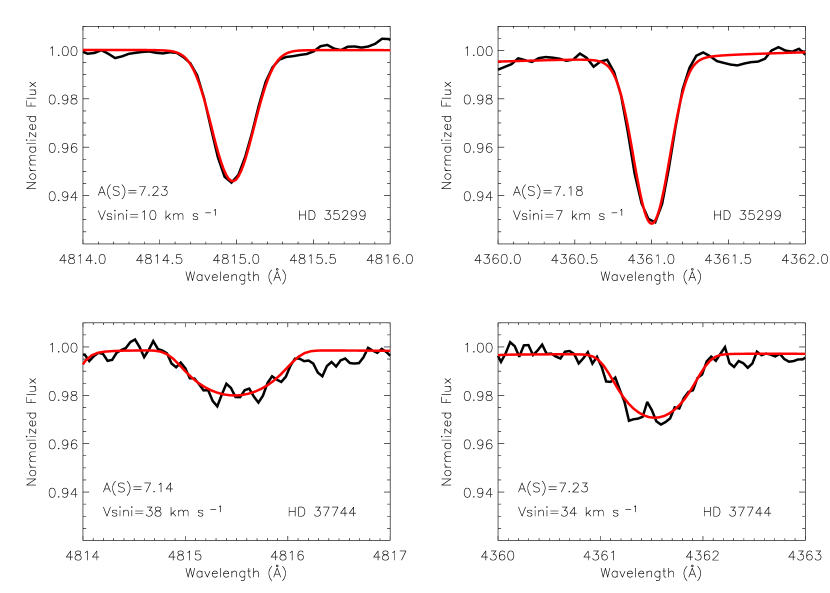
Figure 2: Sample fits showing synthetic profiles (red line) and observed spectra (black line) of a S ii line at 4815 Å and a S iii line at 4361 Å for the target stars HD 35299 and HD 37744. The best-fit $V\sin i$ and abundance values for each line are shown in the panels.

Synthetic line profiles were calculated with the code SURFACE (Butler & Giddings, 1985) and assuming Voigt profile functions. These profiles were then broadened by means of convolution with a rotational profile, including both the projected rotational velocity ($V\sin i$), limb darkening, and the instrumental profile. The microturbulence for each star was kept constant while abundances and $V\sin i$’s were allowed to vary. The best fit for each line was obtained from the $\chi^{2}$-minimization of the differences between theoretical and observed profiles. The S ii and S iii transitions analyzed and atomic data (excitation potentials and oscillator strengths) are found in Table 2; the $gf$-values are from the Opacity Project (Cunto & Mendonza, 1992). In Figure 2 we show examples of best-fit synthetic profiles of S ii and S iii lines for the target stars HD 35299 and HD 37744.

Final sulfur abundance results (including S ii and S iii abundances) and $V\sin i$ values for the stars are presented in Table 1: these are the averages for the individual lines and the respective abundance dispersions are also listed (with the number of sulfur lines fitted for each star appearing in brackets). We note that the dispersions presented in the table represent the line-to-line scatter and are not representative of real uncertainties in the derived abundances. The total errors in our abundance analysis are estimated in Section 3.1. As a check, we compared the projected rotational velocities in Table 1 with $V\sin i$’s derived by adopting a calibration by Daflon et al. (2007) of full-widths at half maximum of He i lines at $\lambda\lambda$4026, 4388 and 4471Å measured from a grid of synthetic spectra calculated in non-LTE. The comparison between the $V\sin i$’s obtained from sulfur lines with those using the He lines calibration is shown in Figure 3. We note a very good agreement between the two sets of $V\sin i$ values; except one star (HD 37209) for which the two determinations agree marginally, within the uncertainties ($V\sin i_{Sulfur}=44\pm 8$ km s^-1 and $V\sin i_{Helium}=53\pm 2$km s^-1).

The analysis of sulfur in B stars is aided by the fact that lines from two ionization stages (S ii and S iii) can be observed and this offers the possibility to constrain the effective temperatures from the ionization balance between S ii and S iii. Spectroscopic T_effs, obtained from an agreement between the abundances from S ii and S iii lines, can provide an additional check on the adopted effective temperature scale for the studied stars (shown in Figure 4). For most stars in our sample, sulfur abundances derived from S ii and S iii lines (adopting the T_eff-scale from Cunha & Lambert 1994) were found to agree within $<$ 0.10 dex. We note however, that the stars HD 36351, HD 36591, and HD 37744 yielded differences in A(S iii $-$ S ii) of +0.20 dex, +0.16 dex and $-0.17$ dex, respectively. The strength of the S ii lines reaches a maximum around T_eff=18,000–19,000 K, whereas the S iii lines are more sensitive to T_eff variations in this temperature range (See figures 7 - 10 of Vrancken et al. 1996). It is likely that the differences between the abundances derived from S ii and S iii lines result from uncertainties in the adopted temperatures. We thus revised the effective temperatures of these three stars by +2.6%, +2% and $-$2%, respectively, in order to bring S ii and S iii abundances into agreement. The $\log g$ values for these stars were also revised in order to obtain similar theoretical fits to the H_γ profiles. These revised T_eff and $\log g$ values and the respective abundance results are listed in Table 1.

Sulfur abundance results for the Orion stars are plotted as a function of the adopted effective temperature in the upper panel of the Figure 5. The effective temperatures of the stars in this sample encompass the range roughly between 20,000K–27,000K and, although for B stars this represents a relatively broad range in T_eff, no trends with abundance are observed. The flat distribution of sulfur abundances derived suggests that these results are probably free of major systematics within this T_eff range. In the lower panel of Figure 5, we present the difference between the abundances derived from S iii and S ii lines (A(S iii $-$ S ii)) also plotted as a function of the adopted T_eff. The differences are small, $<$ $\sim$0.10 dex, and do not show a significant trend with the effective temperature.

In order to briefly evaluate the importance of adopting a treatment in non-LTE versus LTE when studying sulfur abundances in B-type stars, we computed LTE abundances for one target star HD 35299 with T_eff=24,000 and $\log g$=4.25. The results from this test calculation indicate a modest correction for the average abundance of S ii lines: $\delta$ (S ii)${}_{NLTE}-$ (S ii)${}_{LTE}=-0.03$dex. This is a small effect in the average abundance but the S ii line-to-line scatter in LTE is found to be much larger ($\sim$ 0.25 dex) than in non-LTE ($\sim$ 0.15 dex). It should be noted that some of the S ii lines, such as $\lambda$ 4278.5Å, have significant non-LTE corrections ($\sim-$0.7 dex); while others, such as $\lambda$ 4269.7Å and $\lambda$ 4294.4 Å  have relatively small non-LTE corrections ($\sim$ +0.04 dex). A reduced S ii scatter in the average non-LTE abundance as opposed to LTE generally indicates that there is good consistency in the non-LTE calculations of individual lines and adequacy of the adopted model atom. The non-LTE corrections for the S iii lines studied here are also not significant: $\delta$ (S iii)${}_{NLTE}-$ (S iii)${}_{LTE}=-0.02$dex; the line-to-line S iii scatter both in LTE and non-LTE are found to be quite small.

3.1 Abundance Uncertainties

The abundance results in this study are based on a spectrum synthesis analysis and are subject to uncertainties arising mainly from the uncertainties in stellar parameters, microturbulent velocities, as well as placement of the continuum and gf-values. In order to estimate the errors in the derived sulfur abundances, we re-computed the abundances for HD 35299 (a sharp-lined star with T${}_{\rm eff}\sim$24,000K) by independently increasing each of the following parameters, one at a time, by: 4% for T_eff; 0.1 dex for $\log g$; 1.5 km s^-1 for microturbulence; 0.5% for the continuum location and 10% for gf-values. The sensitivity of the sulfur abundances to variations in these parameters are presented in Table 3. The combined errors in the derived S ii and S iii abundances are 0.11 dex and 0.10 dex, respectively.

The stellar parameters in this study were taken from Cunha & Lambert (1994) and these were obtained from an approach which combined Strömgren photometry and LTE theoretical profile fits to the H_γ line wings (Section 3). The adoption of LTE model profiles likely overestimates $\log g$s, in particular for hotter stars with T${}_{\rm eff}\sim$30,000K (Nieva & Przybilla, 2007). For the effective temperature range of the target stars, however, this effect is probably within the uncertainties in the determinations. In order to quantify the errors in log g we did test calculations by re-deriving $\log g$s for 2 target stars (the coolest and the hottest in our sample) using NLTE thoretical profiles of H_γ calculated with DETAIL and SURFACE (Butler 2000, private communication). The results obtained indicate that the differences between ($\log g_{\rm LTE}$ - $\log g_{\rm NLTE}$) vary between 0.05 dex (for the coolest star in our sample) and 0.1 dex (for the hottest star in our sample). Such differences in $\log g$ would result in sulfur abundance differences between $-$0.01 and $-$0.02 dex, at most (Table 3).

4 Discussion

Non-LTE sulfur abundances are derived here for a sample of young B stars from the Orion association: the abundance distribution obtained in this study is homogeneous with a relatively small scatter which is roughly of the order of the abundance errors. The average sulfur abundance for our sample is A(S)= 7.15$\pm$0.05. In the following section we will compare these results with the solar abundance.

4.1 Sulfur Abundances in Orion and the Solar Value

In recent years, the sulfur abundance which is recommended for the Sun has been revised downward by $\sim$0.15–0.20 dex (see, for example, Lodders et al. 2009). The compilation of Solar System abundances by Grevesse & Sauval (1998) listed a photospheric abundance of A(S)= 7.33$\pm$0.11. More recently, Asplund et al. (2006) did a critical evaluation of sample S i lines and removed those lines which were deemed to be blended. This study recommended a lower sulfur abundance of A(S)=7.14 $\pm$ 0.05 for the solar photosphere, in much better agreement with measurements in meteorites (A(S)=7.17 $\pm$ 0.02, Lodders et al. 2009). Note that the photospheric abundances discussed above were obtained using 1-D model atmospheres. An important confirmation of the 1-D result comes from the recent modelling of the forbidden [S i] line at 1082nm by Caffau & Ludwig (2007), which is based on 3-D hydrodynamical model atmospheres, that finds a sulfur abundance extremely consistent with the 1-D results: A(S)= 7.15$\pm(0.01)_{stat}\pm(0.05)_{sys}$.

The average sulfur abundance of the Orion B stars obtained here is found to be in perfect agreement with the Solar System value: the abundances all cluster around A(S)=7.15. Such an agreement, taken at face value, indicates that a non-measurable evolution of the sulfur abundances has taken place in the last $\sim$4.5 Gyrs. The consistency between the sulfur abundances measured for Orion and the Sun (both from 1-D and 3-D model atmospheres and meteorites) also argues favorably for the recent claim by Cunha et al. (2006) and Lanz et al. (2008) that the abundances of Ne and Ar measured in the Orion association can be considered as good proxies for the Solar System abundances; this connection is especially interesting in the case of noble gases because the solar abundances of such elements are much more uncertain, yet these abundances need to be defined as they affect solar interior models.

4.2 Previous Results for Early-Type Stars

Recent studies of chemical abundances in OB stars have not analyzed sulfur (e.g. Pryzbilla et al. 2008; Simon-Diaz et al. 2006) and most of the sulfur abundances which are available in the literature are based on LTE treatments. For example, Gies & Lambert (1992) presented a detailed LTE analysis for a sample of early-type B stars focusing on CNO, but also derived S ii abundances for the coolest B stars in their sample (with T_eff $<$ 24,750K). The mean S abundance in that study is A(S)= $7.21\pm 0.12$, with a slight increase in the abundance as a function of effective temperature that could be explained in terms of the expected errors. On the other hand, Kilian (1994) analyzed a sample of seven stars in the Orion association and obtained $<A(S)>_{LTE}=6.80\pm 0.25$. Their derived abundances show a trend with the effective temperature, and the authors suggest this may result from neglecting non-LTE effects in their analysis.

Line formation in non-LTE was considered in the study by Vrancken et al. (1996). The focus in that paper was on the construction and description of a fairly complete sulfur model atom (which is adopted in the present analysis), but the authors also derived abundances for three B stars as a test of their model atom, for which they obtained sulfur abundances in the range A(S)=7.14 – 7.38. One of the stars studied in that paper, in particular, is also in our sample, HD 37356. For this star, they obtained A(S) = $7.14\pm 0.16$ (considering only S iii lines), in full agreement with A(S) = $7.13\pm 0.14$, obtained here from 13 S ii and 3 S iii lines. More recently, Morel et al. (2006) used the same methodology as in Vrancken et al. (1996) and analyzed sulfur abundances (along with other elements) in a sample of nine $\beta$ Cephei stars. The average sulfur abundances found was A(S)=7.21 $\pm$ 0.13. The results from this sample was later combined with sulfur abundances of 11 stars (not all $\beta$ Cephei; Morel et al. 2008) and the average sulfur abundance obtained is A(S)=7.18 $\pm$ 0.11. We note, however, that the results obtained for Cepheid stars (Andrievsky et al., 2002) are significantly higher than the above: the average sulfur abundance calculated for a sample of 24 Cepheids in the solar neighborhood (located within 7.6 and 8.2 kpc from the Galactic center) is A(S)=7.44 $\pm$ 0.09.

The first systematic non-LTE abundance analysis of sulfur in a large sample of OB stars is presented in the series of papers by Daflon et al. (2003, 2004a, 2004b). The sulfur abundances in these previous studies from our team, however, were based only on two weak S iii lines at 4361 and 4364Å, which fall close to the edge of the red wing of $H_{\gamma}$. It should be noted that for the majority of their targets, the S iii line at 4364Å was the $\it{only}$ measured line, even for target stars with the lowest $V\sin i$s and having spectra with the highest signal-to-noise ratios. The target sample analyzed in these studies covered mostly the solar neighborhood and the inner Galactic disk (galactocentric distances $R_{g}$ between $\sim$ 5–9 kpc) but also included 4 more distant targets ($R_{g}\sim$ 9–14 kpc) which helped in the definition of disk metallicity gradients as discussed in Daflon & Cunha (2004).

4.2.1 Sulfur Abundance Gradients

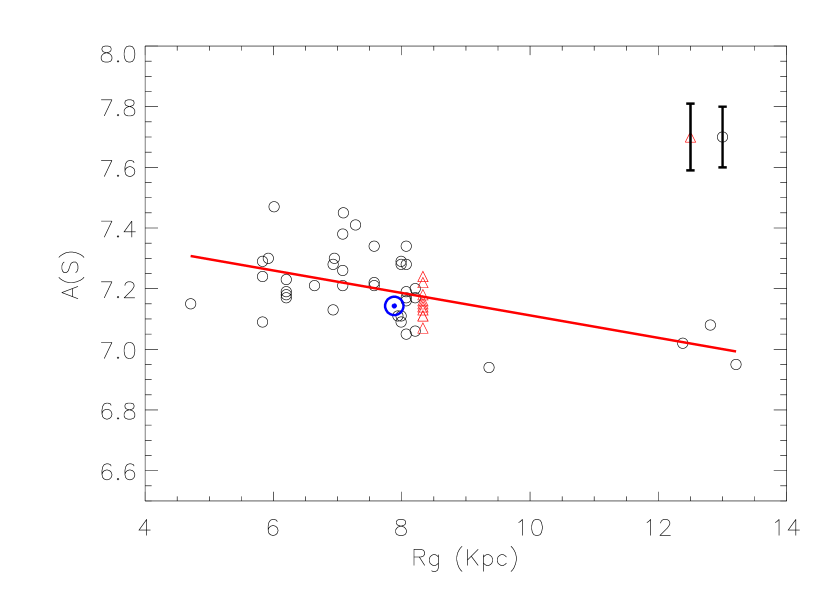
Figure 6: Sulfur abundances plotted as a function of galactocentric distances. The black open circles represent the sample of OB stars studied by Daflon & Cunha (2004); the red open triangles are the Orion abundances for the B stars analyzed in this paper. The Sun is represented at R_g=7.9 Kpc (MacNamara et al., 2000) with $A(S)=7.14$ from Asplund et al. (2006). The sulfur gradient calculated for the entire sample has a slope of $-0.037\pm$0.012 dex Kpc^-1 (shown as the solid red line). The typical errorbars in the abundances are shown in the top right.

The sulfur abundance results from Daflon & Cunha (2004) are shown versus the adopted galactocentric distances in Figure 6 (open circles). The sulfur results for Orion are shown as open triangles and these seem to agree well with the overall trend. The overlap between the abundance results in the solar neighborhood is clear. In particular, if one averages the abundances of all stellar members of the five OB associations located within R_g=7.6–8.2 Kpc, which are Cep OB2, Cep OB3, Cyg OB3, Cyg OB7 and Lac OB1, the average sulfur abundance for this nearby sub-sample is A(S)=$7.19\pm 0.09$: this compares well with the average sulfur abundance obtained for Orion, which is located $\sim$ 500 pc from the Sun, and gives support to previous results (Pryzbilla et al., 2008) that the solar neighborhood abundance is homogeneous, at least at the level of the uncertainties in the abundance analysis.

Such agreement in the abundance results for the solar neighborhood is pleasing since the sulfur abundances derived here are based on several lines from two ionization stages (S ii and S iii), while the previous analyses were obtained from one, or a maximum of two, sulfur lines from a single ionization stage (S iii), and from a different T_eff-scale: the T_effs from Daflon & Cunha (2004) are based on a calibration for the reddening-free parameter Q, and the effective temperatures from Cunha & Lambert (1994) are based on an iteractive scheme that combines photometric calibrations for Strömgren indices and the fitting of H_γ wings.

Since there seems to be no major systematic differences between the sulfur abundances previously published by our group and from this study, the Orion results can be added to compute a new sulfur gradient for the Galactic disk. A linear fit to the run of abundances with distances from the Galactic center is a possible simple description for the overall decrease in the sulfur abundances towards the edge of the disk. The best-fit straight line to the complete dataset in Figure 6 corresponds to $A(S)=(7.481\pm 0.097)-(0.037\pm 0.012)R_{g}$. The adopted distances are from Daflon & Cunha (2004). The sulfur gradient obtained is flat, in line with the previous result obtained by Daflon & Cunha (2004), and very similar to the previously derived oxygen gradient for the same target sample. A similar behavior between sulfur and oxygen is expected as these are both $\alpha$ elements.

4.3 Sulfur Depletion

The Orion Nebula is largely considered as a standard reference for the ionized gas abundances in the local neighborhood (see, for instance, Esteban et al., 2004). However, the direct comparison between the abundance derived for a particular element in the Nebula and in the Sun should consider two important points: first, its depletion onto grains, and second, the effects of the chemical evolution of the solar neighborhood since the Sun was formed. Concerning the evolutionary effects, chemical evolution models by Chiappini et al. (2003) indicate only a small effect, of the order of $\sim$ 0.1 dex, on the sulfur evolution between the formation of the Solar System and the present.

Concerning the more general discussion about the depletion of sulfur onto grains, there are clear indications that sulfur is undepleted in diffuse interstellar gas. Howk et al. (2006) derive a gas-phase sulfur abundance of A(S) = $7.13\pm 0.03$ for the Galactic Halo insterstellar medium. In denser regions, however, the amount of sulfur depletion is not completely clear. Tieftrunk et al. (1994) considered gas-phase abundances in S-bearing molecules and argued that sulfur depletions of factors of $\sim 10^{3}$ could exist. Also, dominant $S^{+}$ ions (of this easily ionized element) can efficiently freeze-out onto negatively charged dust grains in denser regions (Ruffle et al., 1999). Puzzling contrary indications exist, as evidenced by the presence of S ii recombination lines in dense clouds and the absence of strong infrared sulfur features in grains – See Goicoechea et al. (2006) for a discussion. One way to gain insight into this problem is to study Photodissociated Regions (PDR), which are intermediate between diffuse and dark clouds as, for example, the Horsehead PDR (Goicoechea et al., 2006). Even in an environment with large chemical complexity, low sulfur depletion has been found.

In order to constrain the amount of sulfur depletion in the Orion H ii region, one can directly compare the sulfur abundances of young early-type star members of the OB association with the chemical composition of the Orion nebulae, albeit keeping in mind that there may be systematic abundance errors which afflict both the stellar and nebular analysis independently. The chemical composition of the gas which formed the young stars in the Orion association (and which can be measured in the stellar photospheres of OB stars) represents an independent check on the present day gas content, which is measured from nebular lines in its H ii region.

The most recent and detailed study of the chemical composition of the Orion nebulae by Esteban et al. (2004) observed a region near the hot star $\theta^{1}$ Ori, and measured A(S)= $7.22\pm 0.04$; when adopting their preferred value for the temperature fluctuation parameter, $t^{2}$ =0.02 (see Figure 5 showing the results obtained for the young stars in Orion comparison with the dotted line which represents the sulfur abundance for the Orion nebulae from Esteban et al. 2004). Although it should be kept in mind that the stellar and nebular abundances in Orion agree within the quoted errors in the determinations, a brief comparison of the results is of interest. The difference between the nebular and stellar abundances is found to be positive ($\delta$A (S)_Neb-Stel = +0.07 dex) and not explainable as the result of the chemical evolution sulfur as the Orion stars are very young, with ages less than $\sim$ 10 million years. Since the net effect of entrapment of gas onto grains is to reduce the gas phase abundance, the nebular abundance could be viewed as a lower-limit abundance value. If the lowest sulfur abundance value in Esteban et al. (2004) of A(S)=7.06 is adopted, (which corresponds to the extreme case of t²=0.0; not favored by the authors), the amount of sulfur depletion using the B stars as a reference would still be modest or non-existent within the uncertainties. It is easily arguable from these results and their respective uncertainties, that sulfur cannot be significantly depleted in the Orion nebulae.

5 Conclusions

Sulfur abundances are derived in non-LTE for a sample of young B stars of the Orion association. The conclusions from this study are the following:

1. The abundance distribution in Orion is found to be homogeneous within the uncertainties in the analysis. The comparison of sulfur abundances derived for Orion B stars with abundance results for the Sun, the insterstellar medium and early-type stars in the solar vicinity allows us to conclude that the sulfur abundances have undergone very little change from the time of formation of the Solar System $\sim$ 4.5 Gyr ago.

2. The close agreement between the sulfur abundances in Orion and the Sun provides indirect support to previous claims by Lanz et al. (2008) and Cunha et al. (2006) that the young Orion stars can be used as good proxies in order to ascertain the solar abundances of noble gases, such as Ne and Ar, whose abundances are not measurable in the solar photosphere.

3. The abundances of main-sequence B stars overlap with the gas-phase abundance derived by Esteban et al. (2004) for the Orion Nebula. The similarity between these abundances indicates that sulfur is undepleted in the Orion Nebula. Contrary to elements such as C and Fe, for which important depletion exists, sulfur appears to be a remarkably direct metallicity indicator of the Galactic disk (except perhaps in very dense regions).

4. The sulfur abundance results for Orion are added to a database of abundances previously published for OB main sequence stars along the Galactic Disk. The new sulfur abundance gradient computed for a sample of 50 OB stars is $A(S)=(7.481\pm 0.097)-(0.037\pm 0.012)R_{g}$. The sulfur gradient is very similar to the flat gradient of $-0.031\pm 0.012$ dex Kpc^-1 previously obtained for oxygen in Daflon & Cunha (2004) and in agreement with standard chemical evolution model predictions such as Chiappini et al. (2001) and Cescutti et al. (2007).

Table 1: Stellar Parameters and Sulfur Abundances

Star	$T_{{\rm eff}}$	$\log g$	$\xi$	$V\sin i$	A(S ii)	A(S iii)	A(S)
	(K)		(km s-1)	(km s-1)
HD 35039	20550	3.74	8.0	9$\pm$ 1	7.18$\pm$0.16[16]	7.14$\pm$0.13[3]	7.18$\pm$0.15 [19]
HD 35299	24000	4.25	8.0	12$\pm$2	7.12$\pm$0.13[16]	7.06$\pm$0.07[3]	7.11$\pm$0.13 [19]
HD 35912	19590	4.20	8.0	14$\pm$2	7.14$\pm$0.14[15]	7.15$\pm$0.02[2]	7.14$\pm$0.13 [17]
HD 36285	21930	4.40	8.0	14$\pm$2	7.15$\pm$0.13[15]	7.17$\pm$0.10[2]	7.15$\pm$0.13 [17]
HD 36351*	22520	4.23	9.0	31$\pm$4	7.09$\pm$0.10[7]	7.15$\pm$0.01[2]	7.11$\pm$0.09 [9]
HD 36591*	26860	4.26	9.0	11$\pm$2	7.06$\pm$0.03[2]	7.09$\pm$0.11[2]	7.07$\pm$0.07 [4]
HD 36959	24890	4.41	6.0	13$\pm$3	7.13$\pm$0.14[9]	7.24$\pm$0.14[3]	7.16$\pm$0.14 [12]
HD 37209	24050	4.13	10.0	44$\pm$8	7.22$\pm$0.05[5]	7.20$\pm$0.12[2]	7.22$\pm$0.06 [7]
HD 37356	22370	4.13	9.0	20$\pm$3	7.15$\pm$0.14[13]	7.05$\pm$0.14[3]	7.13$\pm$0.14 [16]
HD 37744*	24000	4.35	7.0	38$\pm$4	7.27$\pm$0.14[3]	7.20$\pm$0.04[2]	7.24$\pm$0.11 [5]

Table 2: Atomic Data

Species	Wavelength	$\chi$	$\log gf$
	(Å)	(eV)
Sii	4162.66	15.944	0.789
	4217.18	15.944	$-$0.145
	4269.72	16.092	$-$0.112
	4278.51	16.092	$-$0.111
	4294.40	16.135	0.568
	4463.58	15.944	0.213
	4483.43	15.899	$-$0.064
	4486.63	15.867	$-$0.463
	4524.72	15.068	0.031
	4656.76	13.584	$-$0.519
	4729.44	16.100	$-$0.139
	4815.55	13.672	$-$0.051
	4824.07	16.265	0.062
	5014.07	14.068	0.054
	4991.97	13.617	$-$0.739
	5032.43	13.672	0.157
Siii	4284.88	18.193	$-$0.277
	4361.48	18.244	$-$0.760
	4364.68	18.318	$-$0.846

Table 3: Abundance Uncertainties

	S ii	S iii
$\delta(T_{eff})=+4$%	+0.09	$-0.08$
$\delta(\log g)=+0.1$	+0.02	+0.01
$\delta(\xi)=+1.5$	$-0.04$	$-0.04$
$\delta(gf)=+10$%	+0.04	+0.04
$\delta{\rm(continuum)}=+0.5$%	+0.02	+0.03
$\delta{\rm(total)}$	+0.11	+0.10

Figure 1: Sample observed spectra in the spectral region between 4800–4832Å for all observed targets.

Figure 3: The comparison between projected rotational velocities derived from the fitting of sulfur lines (this study) with $V\sin i$ results based on a calibration of FWHM of theoretical non-LTE He i profiles.

Figure 4: Sulfur abundances of individual S ii (open circles) and S iii (open squares) lines as a function of the ionization potential $\chi$, showing the sulfur ionization balance for the stars HD 35039 (top panel) and HD 36351 (bottom panel). The effective temperatures are from Table 1. The dotted lines represent the mean sulfur abundance for each star.

Figure 5: Top panel: Sulfur abundance results for the sample stars as a function of the adopted effective temperatures. The individual stellar values (filled circles) are the mean sulfur abundances which were obtained from the measured lines and the error bars represent the total errors from Table 3. We also show the abundance measured for the Orion Nebulae by Esteban et al. (2004; dotted line) and the recommended solar value by Asplund et al. (2006; dashed line). Bottom panel: The differences between sulfur abundances derived from S iii and S ii lines as a function of the adopted effective temperatures.

References

- Andrievsky et al. (2002) Andrievsky, S. M.; Kovtyukh, V. V.; Luck, R. E.; Lépine, J. R. D.; Bersier, D.; Maciel, W. J.; Barbuy, B.; Klochkova, V. G.; Panchuk, V. E.; Karpischek, R. U. 2002, A&A 381, 32
- Asplund et al. (2006) Asplund, M., Grevesse, N., & Sauval, A. J. 2006, Nuclear Physics A, 777, 1
- Butler & Giddings (1985) Butler, K., & Giddings, J. R. 1985, in Newsletter on Analysis of Astronomical Spectra, No. 9 (London: Univ. London)
- Caffau et al. (2005) Caffau, E.; Bonifacio, P.; Faraggiana, R.; François, P.; Gratton, R. G.; Barbieri, M. 2005, A&A 441, 533
- Caffau & Ludwig (2007) Caffau, E. & Ludwig, H.-G. 2007, A&A 467, L11
- Cescutti et al. (2007) Cescutti, G., Matteucci, F., François, P., & Chiappini, C. 2007, A&A 462, 943
- Chen et al. (2002) Chen, Y. Q., NIssen, P. E., Zhao, G., & Asplund, M. 2002, A&A 390, 225
- Chiappini et al. (2001) Chiappini, C., Matteucci, F., & Romano, D. 2001, ApJ 554, 1044
- Chiappini et al. (2003) Chiappini, C., Romano, D. & Matteucci, F. 2003, MNRAS 339, 63
- Clayton (2003) Clayton, D. 2003, Handbook of Isotopes in the Cosmos, Cambridge, UK: Cambridge University Press
- Clegg et al. (1981) Clegg, R. E. S.; Tomkin, J., and Lambert, D. L. 1981, ApJ 250, 262
- Cunha & Lambert (1994) Cunha, K. & Lambert, D. L. 1994, ApJ 426, 170
- Cunha et al. (2006) Cunha, K., Hubeny, I.; Lanz, T. 2006, ApJ 647, L143
- Cunto & Mendonza (1992) Cunto, W. & Mendonza, C. 1992, Rev. Mex. Astron. Astrof. 23, 107
- Daflon et al. (2003) Daflon, S., Cunha, K., Smith, V. V., & Butler, K. 2003, A&A 399, 525
- Daflon et al. (2004a) Daflon, S., Cunha, K., & Butler, K. 2004a, ApJ 604, 362
- Daflon et al. (2004b) Daflon, S., Cunha, K., & Butler, K. 2004b, ApJ 606, 514
- Daflon & Cunha (2004) Daflon, S. & Cunha, K. 2004, ApJ 617, 1115
- Daflon et al. (2007) Daflon, S., Cunha, K., de Araújo, F. X., Wolff, S., and Przybilla, N. 2007, AJ 134, .1570
- Esteban et al. (2004) Esteban, C., Peimbert, M., Garcia-Rojas, J., Ruiz, M. T., Peimbert, A., and and Rodriguez, M. 2004, MNRAS 355, 229
- François (1987) François, P. 1987, A&A 176, 294
- François (1988) François, P. 1988, A&A 195, 226
- François et al. (2004) François, P., Matteucci, F., Cayrel, R., Spite, M., Spite, F., & Chiappini, C., 2004 A&A 421, 613
- Garnett (1989) Garnett, D. R. 1989, ApJ 345, 282
- Giddings (1981) Giddings, J. R. 1981, Ph.D. Thesis, Univ. London
- Gies & Lambert (1992) Gies, D. R. & Lambert, D. L. 1992, ApJ 387, 673
- Goicoechea et al. (2006) Goicoechea, J. R., Pety, J., Gerin, M., Teyssier, D., Roueff, E., Hily-Blant, P., & Baek, S. 2006 A&A 456, 565
- Grevesse & Sauval (1998) Grevesse, N. & Sauval, A. J. 1998, Space Sci. Rev. 85, 161
- Howk et al. (2006) Howk, J. C., Sembach, K. R., and Savage, B. D. 2006, ApJ 637, 333
- Israelian & Rebolo (2001) Israelian, G. & Rebolo, R. 2001, ApJ 557, L43
- Kilian (1994) Kilian, J. 1994, A&A 282, 867
- Kurucz (1993) Kurucz, R. 1993, ATLAS9 Stellar Atmosphere Programs and 2 km/s grid. Kurucz CD-ROM No. 13. Cambridge, Mass.: Smithsonian Astrophysical Observatory
- Lanz et al. (2008) Lanz, T., Cunha, K., Holtzman, J. & Hubeny, I. 2008, ApJ 678, 1342
- Lodders et al. (2009) Lodders, K.; Palme, H.; Gail, H. -P. 2009 arXiv09011149
- MacNamara et al. (2000) MacNamara, D. H., Madsen, J. B., Barnes, J. & Ericksen, B. F. 2000, PASP 112, 202
- Morel et al. (2006) Morel, T., Butler, K., Aerts, C., Neiner, C. & Briquet, M. 2006, A&A 457, 651
- Morel et al. (2008) Morel, T.; Hubrig, S.; & Briquet, M. 2008, A&A 481, 453
- Nieva & Przybilla (2007) Nieva, M. F. & Przybilla, N. 2007, A&A 467, 295
- Nissen et al. (2004) Nissen, P. E.; Chen, Y. Q.; Asplund, M.; Pettini, M. 2004, A&A 415, 993
- Nissen et al. (2007) Nissen, P. E.; Akerman, C.; Asplund, M.; Fabbian, D.; Kerber, F.; Kaufl, H. U. & Pettini, M. 2007, A&A 469, 319
- Pryzbilla et al. (2008) Przybilla, N.; Nieva, M. F.; Butler, K. 2008, ApJ 688, L103
- Ryde & Lambert (2004) Ryde, N. & Lambert, D. L. 2004, A&A 415, 559
- Ruffle et al. (1999) Ruffle, D. P., Hartquist, T. W., Caselli, P., & Williams, D. A. 1999, MNRAS 306, 691
- Simón-Díaz et al. (2006) Simón-Díaz, S.; Herrero, A.; Esteban, C.; Najarro, F. 2006, A&A 448, 351
- Takada-Hidai et al. (2002) Takada-Hidai, M., Takeda, Y., Sato, S., Honda, S., Sadakane, K., Kawanomoto, S., Sargent, W. L. W., Lu, L., and Barlow, T. A. 2002, ApJ 573, 614
- Tieftrunk et al. (1994) Tieftrunk, A., Pineau des Forets, G., Schilke, P., & Walmsley, C.M. 1994, A&A 289, 579
- Vrancken et al. (1996) Vrancken, M., Butler, K & Becker, S. R. 1996, A&AS 311, 661