Kernel Spectral Curvature Clustering (KSCC) 

Abstract

Multi-manifold modeling is increasingly used in segmentation and data representation tasks in computer vision and related fields. While the general problem, modeling data by mixtures of manifolds, is very challenging, several approaches exist for modeling data by mixtures of affine subspaces (which is often referred to as hybrid linear modeling). We translate some important instances of multi-manifold modeling to hybrid linear modeling in embedded spaces, without explicitly performing the embedding but applying the kernel trick. The resulting algorithm, Kernel Spectral Curvature Clustering, uses kernels at two levels - both as an implicit embedding method to linearize nonflat manifolds and as a principled method to convert a multi-way affinity problem into a spectral clustering one. We demonstrate the effectiveness of the method by comparing it with other state-of-the-art methods on both synthetic data and a real-world problem of segmenting multiple motions from two perspective camera views.

Supp. webpage: http://www.math.umn.edu/$\sim$lerman/kscc/

1 Introduction

Recently a lot of attention has been focused on multi-manifold modeling [1, 24, 20, 13, 25, 16, 15, 7, 9, 4, 5, 8, 2]. In a typical setting data is sampled from a mixture of distributions approximated by manifolds (e.g., quadratic surfaces in two-view geometries [18]), and the task is to segment the data into different clusters representing the manifolds. This is a common yet challenging problem in many applications such as computer vision, face recognition, and image processing. A well-known example is the clustering of the MNIST handwritten digits [14], where all the images of a given digit live on a distinct manifold.

Due to the nature of manifolds, most algorithms analyze the local geometry of sampled data, such as density, dimension and orientation, and then piece together those local similarities to find the correct clusters [20, 13, 7, 9, 8, 2]. For example, Goldberg et al. [8] estimate local Gaussian models around each data point and apply spectral clustering [17] according to the Hellinger distances between those local models. A different local approach is used by $K$-Manifolds [20], which iteratively clusters data into manifolds via expectation-maximization, i.e., first approximating each cluster by a manifold using a node-weighted multidimensional scaling (while using local neighbors to estimate geodesic distances), and next assigning data points to the closest manifold from the former stage. These methods are sensitive to a number of factors, such as size of local neighborhoods and density of sampled data, and thus are expected to perform poorly when data is sparsely sampled (see e.g., Figs. 2 and 3).

When only flats, i.e., affine subspaces, are used to model the clusters, the corresponding problem, referred to as hybrid linear modeling, is much easier to deal with because there are elegant representations for flats that can be utilized for solving the problem. For example, Generalized Principal Component Analysis (GPCA) [24, 16] uses polynomials to represent linear subspaces, Local Subspace Affinity (LSA) [25] computes an affinity for any pair of points using the distance between their local tangent subspaces and then applies spectral clustering [17], Agglomerative Lossy Compression (ALC) [15] measures the number of bits needed to code the data by general flats (up to a pre-specified distortion), and Spectral Curvature Clustering (SCC) [5, 4] computes a flatness measure for each fixed-size subset of the data. Finally, there are algorithms that use the linear structure and iterate between a data clustering step and a subspace estimation step, e.g., $K$-Flats [12, 11, 3, 23] and Mixtures of Probabilistic PCA (MoPPCA) [21].

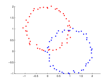
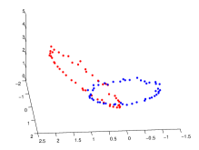
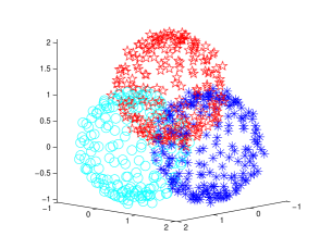
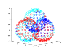
In this work we focus our attention on multi-manifold modeling with parametric surfaces. Our simple but effective idea is to convert the problem into hybrid linear modeling by embedding the underlying (parametric) surfaces into a higher dimensional space where they become flats. For example, when the data is sampled from a union of $(D-1)$-dimensional hyperspheres in the Euclidean space $\mathbb{R}^{D}$, the following function maps them to $D$-dimensional flats in $\mathbb{R}^{D+1}$:

$$\Phi(\mathbf{x})=\begin{pmatrix}\mathbf{x}\\ \left\lVert\mathbf{x}\right\rVert_{2}^{2}\end{pmatrix},\quad\forall\,\mathbf{x}\in\mathbb{R}^{D}.$$ (1)

Fig. 1 illustrates this example for $D=2$. When dealing with parametric surfaces, it is possible to apply hybrid linear modeling algorithms (e.g., [3, 11, 24, 25, 15, 5]) in the embedded space to segment the original manifolds.

Figure 1: Two circles in $\mathbb{R}^{2}$ and their images under the map $\Phi$ (defined in Eq. (1)) in $\mathbb{R}^{3}$.

If a hybrid linear modeling algorithm can be expressed only in terms of the dot products between the data points (e.g., $K$-Flats [12, 11, 3, 23], MoPPCA [21], LSA [25], ALC [15] and SCC [5, 4]), then the explicit embedding can be avoided by using the kernel trick. A kernel is a real-valued function, $k(\mathbf{x},\mathbf{y})$, of two variables $\mathbf{x},\mathbf{y}\in\mathbb{R}^{D}$ such that for any $N$ points $\mathbf{x_{1}},\ldots,\mathbf{x_{N}}$ in $\mathbb{R}^{D}$, the kernel matrix

$$\mathbf{K}:=\{k(\mathbf{x_{i}},\mathbf{x_{j}})\}_{1\leq i,j\leq N}$$ (2)

is symmetric positive semidefinite. It is shown in [19] that any kernel function can be represented as a dot product

$$k(\mathbf{x},\mathbf{y})=\langle\Phi(\mathbf{x}),\Phi(\mathbf{y})\rangle,\quad\forall\,\mathbf{x,y}\in\mathbb{R}^{D},$$ (3)

where $\Phi\colon\mathbb{R}^{D}\rightarrow\mathcal{F}$ and $\mathcal{F}$ is a Hilbert space. The map $\Phi$ is referred to as a feature map and the space $\mathcal{F}$ a feature space. Since we know the desired embedding $\Phi$, we can form the appropriate kernel $k$ by Eq. (3) and replace dot products with $k$ in applicable hybrid linear modeling algorithms.

In this paper we concentrate on the kernelization of the SCC algorithm [4, 5], which we refer to as Kernel Spectral Curvature Clustering (KSCC). The main reason for choosing SCC is that the current implementations of other hybrid linear modeling algorithms that are appropriate for kernelization [21, 3, 11, 25, 15] do not perform sufficiently well on affine subspaces (unlike linear subspaces); see e.g., Fig. 4 and [5, Table 2]. Another important reason is that SCC has established theoretical guarantees [4] and careful numerical estimates [5] which can be used to justify successes and failures of KSCC.

The rest of this paper is organized as follows. We first present the KSCC algorithm in Section 2. Experiments are then conducted in Section 3 to test the algorithm on both artificial data and a real-world problem of two-view motion segmentation (The Matlab codes and relevant data can be found at the supplemental webpage). Finally, Section 4 concludes with a brief discussion and open directions for future work.

2 The KSCC algorithm

Briefly speaking, the KSCC algorithm is the SCC algorithm [4, 5] performed in some user-specified feature space. However, all the relevant calculations in the feature space are accomplished in the original space via the corresponding kernel function. Thus, computations in the possibly high dimensions are avoided so as to save time.

We assume a data set $\mathrm{X}=\{\mathbf{x}_{1},\ldots,\mathbf{x}_{N}\}$ sampled from a collection of $K$ manifolds in $\mathbb{R}^{D}$ (possibly corrupted with noise and outliers). We will represent the data by a mixture of $K$ parametric surfaces of the same model (e.g., general conic sections in $\mathbb{R}^{2}$). Based on the given model of parametric surfaces, we form a feature map $\Phi\colon\mathbb{R}^{D}\rightarrow\mathbb{R}^{L}$ such that the images of the $K$ parametric surfaces are flats (see examples in Section 3). Let $\ell$ be the maximal dimension of the flats. We remark that $\ell$ can be determined by subtracting 1 from the maximal number of affinely independent coordinates of $\Phi$ (though future work will explore substantial reduction of $\ell$, whenever possible, via a feature selection procedure). We then segment the original manifolds by clustering $\ell$-flats, i.e., $\ell$-dimensional flats, in $\mathbb{R}^{L}$. In practice, we use a kernel matrix $\mathbf{K}$ which is implicitly formed by the hidden embedding $\Phi$ according to Eqs. (2) and (3).

The KSCC algorithm starts by computing a polar curvature [5] for any $\ell+2$ points in the feature space via the kernel trick. Roughly speaking, the polar curvature is an $\ell$-dimensional flatness measure (in particular, it is zero for $\ell+2$ points lying on an $\ell$-flat). More formally, it is the $l_{2}$ average of the polar sines at all vertices of the corresponding $(\ell+1)$-simplex in the feature space, multiplied by the diameter of that simplex.

For any set of $\ell+2$ points in the original space with indices $\mathrm{I}=\{i_{1},\ldots,i_{\ell+2}\}$, we denote the corresponding block of the kernel matrix $\mathbf{K}$ by $\mathbf{K}_{\mathrm{I,I}}$ (and similarly later wherever applicable), that is,

$$\mathbf{K}_{\mathrm{I,I}}:=(\mathbf{K}_{ij})_{i,j\in\mathrm{I}}.$$ (4)

The KSCC algorithm computes the polar curvature of their corresponding feature vectors in the following way (see supplementary material for derivation of this formula):

$$c^{2}_{\mathrm{p}}(\mathrm{I}) =\frac{1}{\ell+2}\cdot\max_{i,j\in\mathrm{I}}\left(\mathbf{K}_{ii}+\mathbf{K}_{jj}-2\mathbf{K}_{ij}\right)$$

$$\qquad\cdot\sum_{i\in\mathrm{I}}\frac{\det(\mathbf{K}_{\mathrm{I,I}}+1)}{\prod_{j\in\mathrm{I},j\neq i}\;\mathbf{K}_{ii}+\mathbf{K}_{jj}-2\mathbf{K}_{ij}}.$$ (5)

If any denominator above is zero then the algorithm assigns the value 0 to the polar curvature (this happens only when two points with indices in $\mathrm{I}$ coincide in the feature space).

The KSCC algorithm then assigns to any distinct $\ell+2$ points (with index set $\mathrm{I}$) the following affinity:

$$\mathcal{A}_{\mathrm{p}}(\mathrm{I}) :=e^{-{c^{2}_{\mathrm{p}}(\mathrm{I})/(2\sigma^{2})}},$$ (6)

where $\sigma>0$ is a tuning parameter, and zero otherwise. This function is expected to assign large values (toward 1) for points sampled from the same parametric surface and small values (toward 0) for points sampled from different surfaces. Its computation is solely based on $\mathbf{K}$ without invoking directly the mapping $\Phi$.

The KSCC algorithm next forms pairwise weights $\mathbf{W}$ from the above multi-way affinities:

$$\mathbf{W}_{ij}=\sum_{\mathrm{J}}\mathcal{A}_{\mathrm{p}}(i,\mathrm{J})\cdot\mathcal{A}_{\mathrm{p}}(j,\mathrm{J}),$$ (7)

where the sum is over

$$\{\mathrm{J}=(i_{1},\ldots,i_{\ell+1})\mid 1\leq i_{1},\ldots,i_{\ell+1}\leq N\}.$$ (8)

Finally, it applies spectral clustering [17] (with $\mathbf{W}$) to find the clusters.

We have thus far described the main steps of the KSCC algorithm in theory. However, due to its polynomial complexity ($N^{\ell+2}$), the practical implementation of the algorithm will rely on the numerical strategies developed in [5], in particular, the iterative sampling procedure for estimating the matrix $\mathbf{W}$. This procedure is fundamental to the practical implementation and in fact makes the KSCC a random algorithm, unlike its brief description above. We thus provide its details below.

The zeroth iteration of the iterative sampling starts with a random sample of $c\ll N^{\ell+1}$ $(\ell+1)$-tuples of points from the data $\mathrm{X}$, with index sets $\mathrm{J}_{1},\ldots,\mathrm{J}_{c}$. It then uses them to estimate the weights $\mathbf{W}$ of Eq. (7) as follows:

$$\mathbf{W}_{ij}\approx\sum_{r=1}^{c}\mathcal{A}_{\mathrm{p}}(i,\mathrm{J}_{r})\cdot\mathcal{A}_{\mathrm{p}}(j,\mathrm{J}_{r}).$$ (9)

Based on the above weights, $K$ initial clusters are obtained by spectral clustering [17]. The first iteration then resamples $c/K$ $(\ell+1)$-tuples of points from each of the $K$ previously found clusters to get a better estimate of $\mathbf{W}$ so that $K$ newer (and supposedly better) clusters are found. This procedure is repeated until convergence in order to obtain the best segmentation. We remark that the initial sampling might be critical to good final segmentation and, as $\ell$ becomes larger, it is increasingly difficult to sample enough “useful” $(\ell+1)$-tuples of points at the initial step.

The convergence of iterative sampling is measured by the total kernel least squares error, $e^{2}_{\text{KLS}}$, which sums the least squares errors of $\ell$-flats approximation to the clusters $\mathrm{C}_{1},\ldots,\mathrm{C}_{K}$ in the feature space and can be computed as follows (see supplementary material for proof):

$$e^{2}_{\text{KLS}} =\sum_{k=1}^{K}\sum_{j>\ell}\lambda_{j}(\widetilde{\mathbf{K}}_{\mathrm{C}_{k},\mathrm{C}_{k}}),$$ (10)

where $\lambda_{j}(\cdot)$ denotes the $j$-th largest eigenvalue of the matrix, and $\widetilde{\mathbf{K}}_{\mathrm{C}_{k},\mathrm{C}_{k}}$ is a centered version of $\mathbf{K}_{\mathrm{C}_{k},\mathrm{C}_{k}}$ (the block of the kernel matrix $\mathbf{K}$ corresponding to $\mathrm{C}_{k}$):

$$\widetilde{\mathbf{K}}_{\mathrm{C}_{k},\mathrm{C}_{k}} :=\mathbf{K}_{\mathrm{C}_{k},\mathrm{C}_{k}}-\mathbf{1}_{|\mathrm{C}_{k}|}\cdot\mathbf{K}_{\mathrm{C}_{k},\mathrm{C}_{k}}-\mathbf{K}_{\mathrm{C}_{k},\mathrm{C}_{k}}\cdot\mathbf{1}_{|\mathrm{C}_{k}|}$$

$$\qquad+\mathbf{1}_{|\mathrm{C}_{k}|}\cdot\mathbf{K}_{\mathrm{C}_{k},\mathrm{C}_{k}}\cdot\mathbf{1}_{|\mathrm{C}_{k}|},$$ (11)

in which $|\mathrm{C}_{k}|$ denotes the number of points in $\mathrm{C}_{k}$, and $\mathbf{1}_{n}$ is the $n\times n$ constant matrix with elements $1/n$.

In [5] other numerical strategies, such as an automatic scheme of tuning the parameter $\sigma$, are also developed to speed up the SCC algorithm. We employ the same strategies to boost the performance of the KSCC algorithm and describe the main steps of the resulting algorithm in Algorithm 1.

Algorithm 1 Kernel Spectral Curvature Clustering (KSCC)

0:  Data set $\mathrm{X}$, kernel matrix $\mathbf{K}$, maximal dimension $\ell$ (in feature space), number of manifolds $K$, and number of sampled $(\ell+1)$-tuples $c$ (default = $100\cdot K$)

0:  $K$ disjoint clusters $\mathrm{C}_{1},\ldots,\mathrm{C}_{K}$. Steps:

1:  Sample randomly $c$ subsets of $\mathrm{X}$ (with indices $\mathrm{J}_{1},\ldots,\mathrm{J}_{c}$), each containing $\ell+1$ distinct points.

2:   For each sampled subset $\mathrm{J}_{r}$, compute the squared polar curvature of it and each of the remaining $N-\ell-1$ points in $\mathrm{X}$ by Eq. (2). Sort increasingly these $c\cdot(N-\ell-1)$ squared curvatures into a vector $\mathbf{c}$.

3:   for $p=1$ to $\ell+1$ do • Use Eq. (6) together with $\sigma^{2}=\mathbf{c}(N\cdot c/K^{p})$ to compute the $(N-\ell-1)\cdot c$ affinities and estimate the weights $\mathbf{W}$ via Eq. (9). • Apply spectral clustering [17] to these weights and find a partition of the data $\mathrm{X}$ into $K$ clusters (can follow the corresponding steps of the SCC algorithm [5]). end forRecord the partition $\mathrm{C}_{1},\ldots,\mathrm{C}_{K}$ that has the smallest total KLS error, i.e., $e_{\text{KLS}}$ of Eq. (10), for the corresponding $K$ $\ell$-flats in the feature space.

4:  Sample $c/K$ $(\ell+1)$-tuples of points from each $\mathrm{C}_{k}$ found above and repeat Steps 2 and 3 to find $K$ newer clusters. Iterate until convergence to obtain a best segmentation.

The KSCC algorithm employs kernels at two levels. First, it implicitly maps each data $\mathbf{x}_{i}$ to a feature vector $\mathbf{f}_{i}$ and uses only the kernel matrix to compute the polar curvatures in the feature space. Second, the weight matrix $\mathbf{W}$ (see Eq. (7)) can also be interpreted as a kernel that computes dot products in the space $\mathbb{R}^{N^{\ell+1}}$. Indeed, the feature point $\mathbf{f}_{i}$ is further mapped to the $i$-th slice of the tensor $\mathcal{A}_{\mathrm{p}}$: $\{\mathcal{A}_{\mathrm{p}}(i,i_{1},\ldots,i_{\ell+1}),1\leq i_{1},\ldots,i_{\ell+1}\leq N\}$, which contains the interactions between the point $\mathbf{f}_{i}$ and all $\ell$-flats spanned by any $\ell+1$ points in the feature space.

(a) five circles

(b) three lines and three circles

(c) three (noisy) spheres

(d) three adjacent unit spheres and a plane through their centers

(e) four 1D conic sections

(f) five Lissajous curves

Figure 2: Clusters obtained by the KSCC algorithm on six synthetic data sets.

2.1 Complexity of the KSCC algorithm

The storage requirement of the KSCC algorithm is  $O(N\cdot(D+c))$. The running time is $O(n_{\textrm{s}}\cdot(\ell+1)^{2}\cdot D\cdot N\cdot c)$, where $n_{\textrm{s}}$ is the number of sampling iterations performed.

We briefly explain how to efficiently compute all the $N-\ell-1$ polar curvatures for a fixed $(\ell+1)$-tuple of points (with index set $\mathrm{J}_{r}$) in Step 2 of Algorithm 1. The complexity of computing $\det(\mathbf{K}_{\mathrm{[i\;\mathrm{J}_{r}],[i\;\mathrm{J}_{r}]}}+1)$ for any point $\mathbf{x}_{i}$ in the rest of the data is $O((\ell+2)^{3})$, which would translate into a total cost of $O(N\cdot(\ell+2)^{3})$ for all the $N-\ell-1$ curvatures. However, in any $(\ell+2)$-tuple, $\ell+1$ of the points are the same. Therefore, we can pre-compute all possible determinants of the form $\mathbf{H}_{jk}=\det(\mathbf{K}_{\mathrm{J}_{r}-\{j,k\},\mathrm{J}_{r}-\{j,k\}}+1)$ in $O((\ell+1)^{3})$ time using the fact that $\mathbf{H}=\mathrm{adj}(\mathbf{K}_{\mathrm{J}_{r},\mathrm{J}_{r}}+1)$. Then, each determinant $\det(\mathbf{K}_{\mathrm{[i\;\mathrm{J}_{r}],[i\;\mathrm{J}_{r}]}}+1)$ can be computed in $O((\ell+1)^{2})$ time using its cofactor expansion and the pre-computed minors stored in $\mathbf{H}$, for a total cost of $O(N\cdot(\ell+1)^{2})$, since $\ell\ll N$.

3 Numerical experiments

3.1 Artificial data

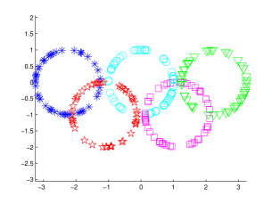
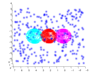
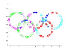
To test the KSCC algorithm we have applied it to several artificial data sets shown in Fig. 2.

In Figs. 2(a)-2(d) the data points lie on circles/spheres and possibly also on lines/planes. We apply the KSCC algorithm with the spherical kernel

$$k_{\mathrm{s}}(\mathbf{x},\mathbf{y})=\mathbf{x}^{\prime}\cdot\mathbf{y}+\left\lVert\mathbf{x}\right\rVert_{2}^{2}\cdot\left\lVert\mathbf{y}\right\rVert_{2}^{2},$$ (12)

which directly follows from Eqs. (1) and (3). We note that $\ell=D$ (clearly, the $D+1$ coordinates of the mapping $\Phi$ in Eq. (1), i.e., $\mathbf{x}_{1},\ldots,\mathbf{x}_{D},\left\lVert\mathbf{x}\right\rVert^{2}_{2}$, are affinely independent).

In Fig. 2(e) the data consists of a circle, an ellipse, a parabola, and a hyperbola. It is natural to use the full quadratic polynomial kernel

$$k_{\textrm{2f}}(\mathbf{x},\mathbf{y})=(1+\mathbf{x}^{\prime}\cdot\mathbf{y})^{2}.$$ (13)

This is equivalent to embedding data by the feature map

$$\Phi(x_{1},x_{2})=(1,\sqrt{2}x_{1},\sqrt{2}x_{2},x_{1}^{2},x_{2}^{2},\sqrt{2}x_{1}x_{2}).$$ (14)

Therefore, the images of the 1-D conics are 4-flats in $\mathbb{R}^{6}$ (the first coordinate of $\Phi$ is constant, so that only the last five coordinates of $\Phi$ are affinely independent). The KSCC algorithm successfully separates the different conic sections.

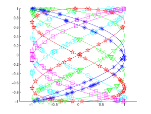
Fig. 2(f) shows five Lissajous curves in the unit square. A Lissajous curve is the graph of the system of parametric equations

$$x=A\sin(at+\delta),\quad y=B\sin(bt).$$ (15)

We have required that $\frac{a}{b}=2$ in Fig. 2(f). In this case, the kernel function can be constructed as follows (see supplementary material for proof):

$$k((x_{1},y_{1}),(x_{2},y_{2}))$$

$$\quad=(1+T_{1}(x_{1})\cdot T_{1}(x_{2})+T_{2}(y_{1})\cdot T_{2}(y_{2}))^{2},$$ (16)

where $T_{n}$ is the Chebyshev polynomial of degree $n$. The KSCC algorithm is then applied with $\ell=4$ in order to separate the curves.

We have also tried to apply other competing algorithms to the data in Fig. 2. Those algorithms are divided into two categories.

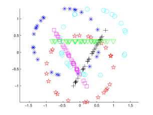
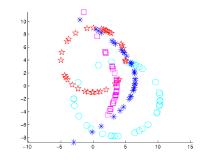
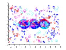
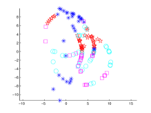
The first category is local algorithms (e.g., [20, 13, 9, 8, 2]), i.e., algorithms that are based on local geometries. Due to the fact that most of the data sets (in Fig. 2) are sparsely sampled and consist of intersecting clusters, these methods would surely fail. In addition, they are generally not suitable for segmenting manifolds using a pre-specified model. Fig. 3 shows the failure of one such algorithm, $K$-Manifolds [20], on the two most densely sampled data sets (Figs. 2(c) and 2(d)). We observed in experiments that the $K$-Manifolds algorithm tends to find arbitrary smooth manifolds that are far from the underlying models.

Figure 3: Demonstration of failure of local algorithms on data sets in Fig. 2.

(a) GPCA (in feature space)

(b) LSA (in feature space)

Figure 4: Demonstration of failure of other hybrid linear modeling algorithms when applied to the data of Fig. 2 in embedded spaces.

The second category is other hybrid linear modeling algorithms, such as $K$-Flats [12, 11, 3, 23], MoPPCA [21], GPCA [24, 16], LSA [25], and ALC [15]. They can be applied to segment the manifolds in Fig. 2 in the same feature spaces as those corresponding to KSCC, where the manifolds are mapped to flats. However, since all these methods do not perform well on general affine subspaces, their performance on the data in Fig. 2 (in feature space) is expected to be very poor.

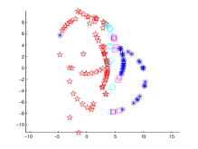
We first applied GPCA and LSA to all data sets in Fig. 2 (after being mapped to affine subspaces), and obtained that the segmentation errors were all around 50%. Fig. 4 shows their segmentation results on two data sets in Fig. 2. We also applied ALC, $K$-Flats and MoPPCA to all the data sets (in Fig. 2) in the feature spaces. We found that the number of clusters found by ALC is very sensitive to its tuning parameter ($\epsilon$), and even when ALC found the correct number of clusters, the clusters were far from the truth. For both MoPPCA and $K$-flats, we used ten restarts (but only recorded the best result), and still observed that the results were all very bad. For fair comparison, we also directly applied the SCC algorithm [5] in the same feature spaces and found that it succeeded on each data set in Fig. 2.

3.2 Two-view motion segmentation

In this section we compare the performance of the KSCC algorithm with one competing method on 13 real data sequences that are studied in [18] (and references therein): (1) boxes; (2) carsnbus3; (3) deliveryvan; (4) desk; (5) lightbulb; (6) manycars; (7) man-in-office; (8) nrbooks3; (9) office; (10) parking-lot; (11) posters-checkerboard; (12) posters-keyboard; and (13) toys-on-table. Each sequence consists of two image frames of a 3-D dynamic scene taken by a perspective camera (see Fig. 5), and the task is to separate the trajectories of some feature points (tracked on the moving objects) in the two camera views of the scene. This application lies in the field of structure from motion, which is one of the fundamental problems in computer vision.

(a) parking-lot

(b) office

Figure 5: Two sample sequences.

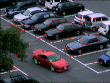
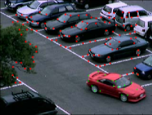
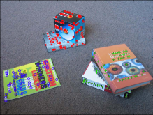
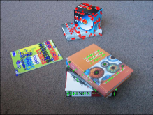
Given a point $\mathbf{x}\in\mathbb{R}^{3}$ in space and its image correspondences $(x_{1},y_{1})^{\prime},(x_{2},y_{2})^{\prime}\in\mathbb{R}^{2}$ in two views, one can form a joint image sample $\mathbf{y}=(x_{1},y_{1},x_{2},y_{2},1)^{\prime}\in\mathbb{R}^{5}$. It is shown (e.g., in [18]) that, under perspective camera projection, all the joint image samples $\mathbf{y}$ corresponding to one motion live on a distinct quadratic manifold in $\mathbb{R}^{5}$. More precisely, for a 3-D rigid-body motion, there exists a symmetric 5-by-5 matrix

$$\mathbf{H}=\begin{pmatrix}0&0&h_{1}&h_{2}&h_{3}\\ 0&0&h_{4}&h_{5}&h_{6}\\ h_{1}&h_{4}&0&0&h_{7}\\ h_{2}&h_{5}&0&0&h_{8}\\ h_{3}&h_{6}&h_{7}&h_{8}&h_{9}\end{pmatrix}$$ (17)

such that

$$\mathbf{y}^{\prime}\cdot\mathbf{H}\cdot\mathbf{y}=0;$$ (18)

and for a 2-D planar motion, there exist three matrices $\mathbf{H}_{1},\mathbf{H}_{2},\mathbf{H}_{3}$ of the same form as in Eq. (17), such that

$$\mathbf{y}^{\prime}\cdot\mathbf{H}_{i}\cdot\mathbf{y}=0,\quad i=1,2,3.$$ (19)

This fact has been used by the Robust Algebraic Segmentation (RAS) algorithm [18] for constructing the perspective Veronese map in order to segment the motions.

To solve the two-view motion segmentation problem, we also apply the above result but will show that each motion uniquely determines a 7-flat (for 3-D rigid-body motion) or 5-flat (for 2-D planar motion) in the space $\mathbb{R}^{9}$ and that KSCC can be applied to the original 4-D point correspondences $(x_{1},y_{1},x_{2},y_{2})$ via a properly constructed kernel function. Indeed, if we define $\mathbf{z}:=(x_{1},y_{1},1)\otimes(x_{2},y_{2},1)$, where $\otimes$ denotes the Kronecker product, then Eq. (18) can be rewritten into a linear equation as follows:

$$\mathbf{z}\cdot(2h_{1},2h_{2},2h_{3},2h_{4},2h_{5},2h_{6},2h_{7},2h_{8},h_{9})^{\prime}=0,$$ (20)

and Eq. (19) into three such linear equations.

Therefore, if the 4-D point correspondences $(x_{1},y_{1},x_{2},y_{2})$ are mapped to the 9-D feature vectors $\mathbf{z}$, then one can segment the motions by clustering 7-flats and 5-flats in $\mathbb{R}^{9}$ (the last coordinate of $\mathbf{z}$ is constant). We follow the same idea of SCC [5] to use only the maximal dimension when having mixed dimensions, which seems to be effective in many cases. Therefore, we apply the KSCC algorithm with $\ell=7$, together with the following kernel function:

$$k\left((x_{1},y_{1},x_{2},y_{2}),(u_{1},v_{1},u_{2},v_{2})\right)$$

$$\quad=\left((x_{1},y_{1},1)\otimes(x_{2},y_{2},1)\right)\cdot\left((u_{1},v_{1},1)\otimes(u_{2},v_{2},1)\right)^{\prime}$$

$$\quad=(x_{1}u_{1}+y_{1}v_{1}+1)\cdot(x_{2}u_{2}+y_{2}v_{2}+1).$$ (21)

We use the outliers-free version of the 13 data sets from [18] in order to solely focus on the clustering aspect. We apply the KSCC algorithm (with the default $c$) to each sequence and record the misclassification rate (in percentage) and the running time (in seconds). To mitigate the effect of randomness due to initial sampling, we repeat this experiment 200 times and compute a mean error $e_{\mathrm{mean}}$, a standard deviation $e_{\mathrm{std}}$, as well as an average running time $t$. We have also applied the RAS algorithm [18] to these outlier-free data, and found that RAS relies on an angleTolerance parameter (the output was quite sensitive to choices of this parameter). We tried a few different values and combined the results into a coherent clustering. All the experiments were performed on an IBM T43p laptop with a 2.13 GHz Intel Pentium M processor and 1 Gb of RAM. The results obtained by the two algorithms are summarized in Table 1 (note that the results of RAS are not reported in [18]).

Table 1: The misclassification rates (in percentage) and the running times (in seconds) of the KSCC and RAS algorithms when applied to the 13 sequences. The second column presents the number of samples $N$ in each sequence. Due to randomness, the KSCC algorithm is applied 200 times to each sequence, and a mean $e_{\mathrm{mean}}$ and a standard deviation $e_{\mathrm{std}}$ of the errors are computed.

		KSCC			RAS
Seq.	$N$	$e_{\mathrm{mean}}$	$e_{\mathrm{std}}$	$t$	$e$	$t$
1	236	0.85%	0.00%	2.14	0.85%	6.68
2	219	1.04%	5.63%	2.05	0.00%	6.68
3	254	30.8%	5.59%	2.59	15.4%	6.84
4	155	0.22%	1.04%	1.99	5.16%	4.50
5	205	0.00%	0.00%	1.86	0.00%	5.29
6	144	15.7%	8.96%	0.70	0.00%	3.91
7	73	0.63%	2.76%	1.87	15.1%	1.17
8	388	1.97%	5.45%	3.43	11.1%	20.2
9	259	0.05%	0.13%	2.18	0.00%	6.68
10	136	22.3%	18.7%	1.18	0.00%	2.89
11	280	4.97%	1.03%	2.68	0.00%	10.5
12	297	1.38%	0.80%	2.62	0.34%	9.49
13	91	2.89%	3.78%	0.87	18.7%	1.84

We observe that the KSCC and RAS algorithms (a) obtain the same classification error on sequences 1, 5, 9 (on sequence 9 the difference is negligible: $0.05\%\cdot 259=0.13$); (b) have significantly different misclassification rates (i.e., with a difference larger than 4%) on eight sequences (3, 4, 6, 7, 8, 10, 11, 13), with each algorithm having a better performance on four of them (KSCC on sequences 4, 7, 8, 13, and RAS on sequences 3, 6, 10, 11); (c) have very small difference on sequences 2, 12 (about 1%, i.e., 3 points). In terms of running time, the KSCC algorithm is at least twice as fast as RAS on all sequences (except sequence 7), sometimes even being five times faster (on sequence 8). In summary, the KSCC and RAS algorithms have almost comparable performances in terms of segmentation errors; however, the KSCC algorithm is faster.

4 Discussions and future work

We have combined the SCC algorithm [5] and kernels to suggest the KSCC algorithm (Algorithm 1) for segmenting parametric surfaces which can be mapped to flats in spaces of moderate dimensions. The computational task is performed solely in the original data space (using the kernel matrix), thus one would expect KSCC to be faster than performing SCC in the embedded spaces (when having large dimensions). We have exemplified its success on a few artificial instances of multi-manifold modeling and on a real-world application of two-view motion segmentation under perspective camera projection.

There are several important issues that need to be further explored in order to more broadly and successfully apply the KSCC algorithm.

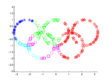
1) The choice of the kernel function might affect the success of the KSCC algorithm. We exemplify this on the three-sphere data in Fig. 2(c), where we used the spherical kernel (see Eq. (12)) and practically segmented $3$-flats in $\mathbb{R}^{4}$. We now apply KSCC to the same data with the following two choices of kernels: the standard quadratic polynomial kernel

$$k_{\textrm{2s}}(\mathbf{x},\mathbf{y})=\langle\mathbf{x},\mathbf{y}\rangle+\langle\mathbf{x}.^{2},\mathbf{y}.^{2}\rangle,$$ (22)

where $.^{2}$ means taking elementwise squares, and the full quadratic polynomial kernel $k_{\textrm{2f}}(\cdot,\cdot)$ of Eq. (13), respectively. This is equivalent to applying SCC to segment $5$-flats in $\mathbb{R}^{6}$ and $8$-flats in $\mathbb{R}^{9}$, respectively. The corresponding results are shown in Fig. 6.

Figure 6: Output of the KSCC algorithm when applied to the three spheres in Fig. 2(c) with the two kernels $k_{\textrm{2s}}$ and $k_{\textrm{2f}}$, respectively.

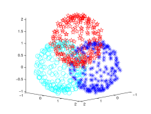
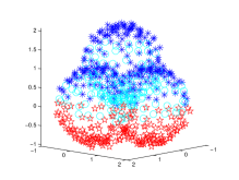
As it turned out, the KSCC algorithm failed with the full quadratic kernel $k_{\textrm{2f}}$. The reason for this is that as $\ell$ increases, the segmentation task becomes more difficult for KSCC since the initial approximation of the weight matrix $\mathbf{W}$ (defined in Eq. (7)) would deteriorate. This experiment suggests that one should use the optimal kernel function with KSCC in the sense that it should minimize the intrinsic dimension of the flats in the feature space. We are currently developing an automatic scheme to choose the least number of terms that are necessary for linearization of the manifolds.

2) The dimension of the flats in the feature space is often quite large, sometimes even with the optimal kernel function (for example, $\ell=25$ in the problem of segmenting motions from three perspective camera views [10]). Due to the limitation of the KSCC algorithm in dealing with large $\ell$, a better initialization strategy needs to be explored in order to more robustly estimate the initial weights $\mathbf{W}$. We plan to develop such a technique in later research and consequently apply the improved KSCC algorithm to solve the three-view motion segmentation problem [10].

3) We need to examine more carefully the situation when data is corrupted with noise. Though KSCC can handle small levels of noise, the clustering task becomes very challenging for KSCC (and probably for any other manifold clustering algorithm) when the noise level increases in the original space. There are two reasons for this. First, in many cases the manifold structure obscures quickly when corrupted with noise (see e.g., Figs. 2(b) and 2(e)). Second, the noise level is further enlarged in feature space due to the embedding having higher-order terms. One has to develop theoretical guarantees for good performance of KSCC in the presence of noise (as done for SCC in [4]), and use related insights for improving the current algorithm. For example, one can note the effect of special geometric transformations of the data, under which the noise distortion (from original to feature space) is minimal, and apply them before the KSCC algorithm.

4) We need to study the performance of KSCC on data contaminated with outliers. Solutions can follow the idea used in the SCC algorithm [5] and possibly combined with RANdom SAmple Consensus (RANSAC) [6, 22, 26], in a similar way as the RAS algorithm [18]. Future work will test the KSCC algorithm on the 13 data sets (in Table 1) in the presence of outliers.

References

- [1] S. Agarwal, J. Lim, L. Zelnik-Manor, P. Perona, D. Kriegman, and S. Belongie. Beyond pairwise clustering. In Proceedings of the 2005 IEEE Computer Society Conference on Computer Vision and Pattern Recognition (CVPR’05), volume 2, pages 838–845, 2005.
- [2] E. Arias-Castro, G. Chen, and G. Lerman. Spectral Clusteirng based on Local Polynomial Approximations. In preparation.
- [3] P. Bradley and O. Mangasarian. k-plane clustering. J. Global optim., 16(1):23–32, 2000.
- [4] G. Chen and G. Lerman. Foundations of a multi-way spectral clustering framework for hybrid linear modeling. Found. Computat. Math. (online), 2009. DOI 10.1007/s10208-009-9043-7.
- [5] G. Chen and G. Lerman. Spectral curvature clustering (SCC). Int. J. Comput. Vision, 81(3):317–330, 2009.
- [6] M. Fischler and R. Bolles. Random sample consensus: A paradigm for model fitting with applications to image analysis and automated cartography. Comm. of the ACM, 24(6):381–395, June 1981.
- [7] A. Goh and R. Vidal. Clustering and dimensionality reduction on Riemannian manifolds. In CVPR, pages 1–7, Anchorage, AK, 2008.
- [8] A. Goldberg, X. Zhu, A. Singh, Z. Xu, and R. Nowak. Multi-manifold semi-supervised learning. In Twelfth International Conference on Artificial Intelligence and Statistics (AISTATS), 2009.
- [9] G. Haro, G. Randall, and G. Sapiro. Translated Poisson mixture model for stratification learning. Int. J. Comput. Vision, 80(3):358–374, 2008.
- [10] R. Hartley and R. Vidal. The multibody trifocal tensor: Motion segmentation from 3 perspective views. IEEE Computer Society Conference on Computer Vision and Pattern Recognition.
- [11] J. Ho, M. Yang, J. Lim, K. Lee, and D. Kriegman. Clustering appearances of objects under varying illumination conditions. In Proceedings of International Conference on Computer Vision and Pattern Recognition, volume 1, pages 11–18, 2003.
- [12] A. Kambhatla and T. Leen. Fast non-linear dimension reduction. In Advances in Neural Information Processing Systems 6, pages 152–159, 1994.
- [13] D. Kushnir, M. Galun, and A. Brandt. Fast multiscale clustering and manifold identification. Pattern Recognition, 39(10):1876–1891, October 2006.
- [14] Y. LeCun and C. Cortes. The MNIST database of handwritten digits. http://yann.lecun.com/exdb/mnist/.
- [15] Y. Ma, H. Derksen, W. Hong, and J. Wright. Segmentation of multivariate mixed data via lossy coding and compression. IEEE Transactions on Pattern Analysis and Machine Intelligence, 29(9):1546–1562, September 2007.
- [16] Y. Ma, A. Y. Yang, H. Derksen, and R. Fossum. Estimation of subspace arrangements with applications in modeling and segmenting mixed data. SIAM Review, 50(3):413–458, 2008.
- [17] A. Ng, M. Jordan, and Y. Weiss. On spectral clustering: Analysis and an algorithm. In Advances in Neural Information Processing Systems 14, pages 849–856, 2001.
- [18] S. Rao, A. Yang, S. Sastry, and Y. Ma. Robust algebraic segmentation of mixed rigid-body and planar motions. Available at http://www.eecs.berkeley.edu/yang/paper/IJCV08-RAS.pdf, 2008.
- [19] B. Schölkopf and A. J. Smola. Learning with Kernels. The MIT Press, Cambridge, Massachusetts, 2002.
- [20] R. Souvenir and R. Pless. Manifold clustering. In the 10th International Conference on Computer Vision (ICCV 2005), 2005.
- [21] M. Tipping and C. Bishop. Mixtures of probabilistic principal component analysers. Neural Computation, 11(2):443–482, 1999.
- [22] P. H. S. Torr. Geometric motion segmentation and model selection. Phil. Trans. R. Soc. Lond. A, 356:1321–1340, 1998.
- [23] P. Tseng. Nearest -flat to points. Journal of Optimization Theory and Applications, 105(1):249–252, April 2000.
- [24] R. Vidal, Y. Ma, and S. Sastry. Generalized principal component analysis (GPCA). IEEE Transactions on Pattern Analysis and Machine Intelligence, 27(12), 2005.
- [25] J. Yan and M. Pollefeys. A general framework for motion segmentation: Independent, articulated, rigid, non-rigid, degenerate and nondegenerate. In ECCV, volume 4, pages 94–106, 2006.
- [26] A. Y. Yang, S. R. Rao, and Y. Ma. Robust statistical estimation and segmentation of multiple subspaces. In Computer Vision and Pattern Recognition Workshop, June 2006.