Critical behavior of the Ising model in annealed scale-free networks

Abstract

We study the critical behavior of the Ising model in annealed scale-free (SF) networks of finite system size with forced upper cutoff in degree. By mapping the model onto the weighted fully connected Ising model, we derive analytic results for the finite-size scaling (FSS) near the phase transition, characterized by the cutoff-dependent two-parameter scaling with four distinct scaling regimes, in highly heterogeneous networks. These results are essentially the same as those found for the nonequilibrium contact process in annealed SF networks, except for an additional complication due to the trivial critical point shift in finite systems. The discrepancy of the FSS theories between annealed and quenched SF networks still remains in the equilibrium Ising model, like some other nonequilibrium models. All of our analytic results are confirmed reasonably well by numerical simulations.

I introduction

Many aspects of our real world have been understood in the context of complex networks NetworkReview ; DorogovtsevBook and simple physical models of critical phenomena on networks. Contrary to regular lattices in the Euclidean space, complex networks are characterized by a highly heterogeneous structure as manifested in broad degree distributions. Recent studies on equilibrium or nonequilibrium systems have revealed that the heterogeneity is one of essential ingredients determining the universal feature of phase transitions and critical phenomena Dorogovtsev2007 .

The concept of the phase transition is well defined only in the thermodynamic limit where the system size is taken to infinity. So it is important to understand how finite-size effects come into play near the transition. Such a task for physical models on regular lattices has been successfully accomplished by the standard finite-size scaling (FSS) theory Privman1990 , based on the ansatz that a single characteristic length scale (correlation length) $\xi$ competes with the system’s linear size $L$. Then, any physical observable depends only on a dimensionless variable $\ell=L/\xi$ in the scaling limit. Near a second-order continuous transition, the correlation length diverges as $\xi\sim|\epsilon|^{-\nu}$ with the reduced coupling constant $\epsilon$ and the finite-size effects become prominent.

The FSS theory for complex networks can be formulated in a similar way: Since the Euclidean distance is undefined in complex networks, one may take the volume scaling variable as ${\ell}_{v}=N/\xi_{v}$ with the system size $N$ (the total number of nodes) and the correlated volume $\xi_{v}$. The correlated volume diverges $\xi_{v}\sim|\epsilon|^{-\bar{\nu}}$ near the transition ($\bar{\nu}=\nu d$ in $d$ dimensional lattices). For example, the magnetization of the Ising model scales as

$$m(\epsilon,N)=N^{-\beta/\bar{\nu}}\psi(\epsilon N^{1/\bar{\nu}}),$$ (1)

where the scaling function $\psi(x)\sim O(1)$ for small $x$ and $x^{\beta}$ for large $x$ with the order parameter exponent $\beta$.

The FSS theory with a single characteristic size has been tested numerically in many systems (see Ref. Dorogovtsev2007 and references therein). In particular, the exact values for the FSS exponent $\bar{\nu}$ are conjectured HHong2007 by estimating the correlated volume (droplet) size for the nonequilibrium contact process (CP) and the equilibrium Ising model in random uncorrelated networks with static links, which are denoted as quenched networks.

However, considering a highly heterogeneous scale-free (SF) network, one should take into account not only a broad degree distribution of $P(k)\sim k^{-\lambda}$ but also the upper cutoff $k_{c}$ in degree, which scales as $k_{c}\sim N^{1/\omega}$. Without any constraint, $k_{c}$ is bounded naturally with $\omega_{\rm nat}=\lambda-1$. In general, one may impose a forced cutoff with $\omega>\omega_{\rm nat}$. In the thermodynamic limit, both $N$ and $k_{c}$ diverge simultaneously and $\omega$ sets a route to the limit. Therefore, one can suspect that the FSS theory may depend on the routes or equivalently on the value of $\omega$, especially for networks with a broader distribution for small $\lambda$.

For the quenched SF networks, it has been suggested that the FSS does not vary with $\omega$ for a weak forced cutoff ($\omega<\lambda$), which was confirmed numerically in various types of SF networks HHong2007 ; Ha2007 . However, in the annealed networks where links are not fixed but fluctuate randomly in time, it was rigorously shown that the CP model exhibits an anomalous FSS for any forced cutoff with $2<\lambda<3$ where a heterogeneity($\lambda$)-dependent critical scaling appears CP-S2007 ; Castellano2007 ; Boguna2009 ; JDNoh2009 . Moreover, the anomalous FSS is characterized by a cutoff($\omega$)-dependent and two-parameter scaling with four distinct scaling regimes JDNoh2009 , in contrast to the cutoff-independent and single-parameter scaling with three scaling regimes in the standard FSS theory.

The anomalous FSS of the CP in the annealed SF networks gives rise to a natural question: What is the main ingredient causing the anomaly? Some possible guesses may be a nonequilibrium feature of the CP, absorbing nature (vanishing activity) at criticality, or heterogeneity of networks Castellano2007 ; Boguna2009 . In this paper, we answer to this question by studying the Ising model, a prototype equilibrium phase transition model, in annealed SF networks. We find the same type of the anomalous FSS scaling (cutoff-dependent and two-parameter scaling with four distinct scaling regimes) for any forced cutoff with $3<\lambda<5$ where the $\lambda$-dependent critical scaling appears in the thermodynamic limit for the Ising version. In addition, the trivial shift of the critical point in finite systems adds one more complication on the critical FSS, though it does not cause any fundamental change. In summary, our results may draw a general conclusion that the anomalous FSS scaling should appear in any critical system in the annealed SF networks for any forced cutoff ($\omega>\omega_{\rm nat}$) with the degree exponent $\lambda$ such that a $\lambda$-dependent new singularity arises in the physical quantities as $N\rightarrow\infty$.

This paper is organized as follows. We define the Ising model on an annealed network in Sec. II and show that it is equivalent to the Ising model on the weighted fully connected network. In Sec. III, the FSS theory is developed in various networks including SF networks, which is numerically tested in Sec. IV. In Sec. V, some effects of the sampling disorder are discussed. We conclude this paper with summary and discussion in Sec. VI.

II Ising model on annealed networks

An annealed network $\mathcal{G}_{N}$ is defined as an ensemble of all networks consisting of $N$ nodes which are assigned to a given degree sequence $\{k_{1},\ldots,k_{N}\}$. An instance $g\in\mathcal{G}_{N}$ is constructed by assigning $k_{i}$ stubs to each node $i~{}(1,\ldots,N)$ and then completing edges by pairing the stubs randomly as in the uncorrelated configuration model Newman2001 ; CBP-S2005 .

A network configuration $g$ is conveniently represented by an adjacency matrix $A(g)$ whose element $A_{ij}$ takes either 1 or 0 if there is an edge between nodes $i$ and $j$ or not, respectively. In the ensemble $\mathcal{G}_{N}$, the connecting probability $p_{ij}$ to find an edge between two nodes $i$ and $j$ is given by Dorogovtsev2007 ; PN2004

$$p_{ij}=\frac{k_{i}k_{j}}{Nz_{1}}+\mathcal{O}\left(\frac{1}{N^{2}}\right),$$ (2)

with the mean degree $z_{1}\equiv\sum_{i}k_{i}/N$. This expansion is valid when $\frac{k_{i}k_{j}}{Nz_{1}}\ll 1$ for all $i$ and $j$.

The ferromagnetic Ising model on the annealed network $\mathcal{G}_{N}$ is defined by the Hamiltonian

$$H[\{s\},g]=-{J}\sum_{i<j}A_{ij}(g)s_{i}s_{j}-\sum_{i}h_{i}s_{i},$$ (3)

where ${J}>0$ is a ferromagnetic coupling constant, $s_{i}\in\{-1,1\}$ is an Ising spin variable at node $i$, and $h_{i}$ is a local field at node $i$. In comparison to the model on a quenched network, a network configuration $g$ is also fluctuating within $\mathcal{G}_{N}$ as well as the Ising spins. Thermodynamic properties of the model is obtained from the partition function

$$Z=\sum_{g\in\mathcal{G}_{N}}\sum_{\{s_{i}\}}\exp\left[{K}\sum_{i<j}A_{ij}(g)s_{i}s_{j}+\sum_{i}\tilde{h}_{i}s_{i}\right],$$ (4)

where ${K}=\beta{J}$ and $\tilde{h}_{i}=\beta h_{i}$ with the inverse temperature $\beta=1/k_{B}T$.

In terms of the connection probability in Eq. (2), one can easily perform the partial summation over $g$ to obtain that

$$Z=\sum_{\{s_{i}\}}\prod_{i<j}\left[(1-p_{ij})+p_{ij}e^{{K}s_{i}s_{j}}\right]\prod_{i}e^{\tilde{h}_{i}s_{i}}.$$ (5)

Utilizing the identity $e^{{K}s}=\cosh{K}+s\sinh{K}$ for $s=\pm 1$, we find that

$$Z=Z_{0}\sum_{\{s_{i}\}}\exp\left(\sum_{i<j}Q_{ij}s_{i}s_{j}+\sum_{i}\tilde{h}_{i}s_{i}\right),$$ (6)

where $Z_{0}$ is an overall constant factor (not depending on $\{s_{i}\}$),

$$Z_{0}=\prod_{i<j}\left(\frac{1-p_{ij}+p_{ij}\cosh K}{\cosh Q_{ij}}\right),$$

and

$$\tanh Q_{ij}=\frac{p_{ij}\sinh{K}}{1-p_{ij}+p_{ij}\cosh{K}}\ .$$ (7)

As $Q_{ij}$ is nonzero for any pair of $(i,j)$, the expression in Eq. (6) corresponds to the partition function of the Ising model on the fully connected network with the heterogeneous coupling constants $Q_{ij}$.

As $p_{ij}=k_{i}k_{j}/(Nz_{1})\ll 1$ for large $N$ exp1 , one can approximate $Q_{ij}\simeq\tilde{K}k_{i}k_{j}/(Nz_{1})$ with $\tilde{K}=\sinh{K}$. Hence, in this paper, we focus on studying the Ising model on the fully connected network with the Hamiltonian $H_{f}$ as

$$\beta H_{f}=-\tilde{K}\sum_{i<j}\frac{k_{i}k_{j}}{Nz_{1}}s_{i}s_{j}-\sum_{i}\tilde{h}_{i}s_{i}.$$ (8)

This Hamiltonian was studied as a MF or annealed approximation for the Ising model on quenched networks in the thermodynamic limit Dorogovtsev2007 ; Bianconi2002 ; Igloi2002 .

For convenience, we rewrite $H_{f}$ in a completed square form as

$$\beta H_{f}=-\frac{\tilde{K}}{2Nz_{1}}\left[\left(\sum_{i}k_{i}s_{i}\right)^{2}-\sum_{i}k_{i}^{2}\right]-\sum_{i}\tilde{h}_{i}s_{i}\$$ (9)

and define the magnetic order parameter as

$$\tilde{M}\equiv\sum_{i}k_{i}s_{i},$$ (10)

with the order parameter density $\tilde{m}\equiv\tilde{M}/(Nz_{1})$, which is first suggested in Dorogovtsev2003 and recently for both equilibrium and nonequilibrium models in Caccioli2009 .

Now we derive the free energy as a function of $\tilde{M}$, which allows us to calculate thermodynamic properties not only in the thermodynamic limit by minimizing it with respect to $\tilde{M}$ but also for finite size $N$, at least up to the leading order. After dropping the additive constant term in Eq. (9), the partition function, up to a constant, can be written as

$$Z = \sum_{\{s_{i}\}}\exp\left[\frac{\tilde{K}}{2Nz_{1}}\left(\sum_{i}k_{i}s_{i}\right)^{2}+\sum_{i}\tilde{h}_{i}s_{i}\right]$$ (11)

$$= \int d\tilde{M}\sum_{\{s_{i}\}}e^{\tilde{K}\tilde{M}^{2}/(2Nz_{1})+\sum_{i}\tilde{h}_{i}s_{i}}\delta\left(\tilde{M}-\sum_{i}k_{i}s_{i}\right)$$

$$= \int d\tilde{M}\int_{-i\infty}^{i\infty}\frac{du}{2\pi i}\exp[-\tilde{F}(\tilde{M},u)]\ ,$$

where

$$\tilde{F}(\tilde{M},u)\equiv-\frac{\tilde{K}}{2Nz_{1}}\tilde{M}^{2}+u\tilde{M}-N\overline{\ln[2\cosh(uk_{i}+\tilde{h}_{i})]},$$

where $\overline{()_{i}}\equiv\frac{1}{N}\sum_{i}()_{i}$ denotes the average over nodes. In obtaining Eq. (11), we used the integral representation of the delta function $\delta(\tilde{M})=\int\frac{dv}{2\pi}e^{iv\tilde{M}}$ and the analytic continuation $v=iu$.

The integration over $u$ can be evaluated using the steepest descent method, which yields that the free-energy function $F(\tilde{M})$ defined by $Z\equiv\int d\tilde{M}\exp(-F(\tilde{M}))$ is given as

$$F(\tilde{M})\simeq\tilde{F}(\tilde{M},u_{0})+\frac{1}{2}\ln\left[2\pi|\tilde{F}^{\prime\prime}|\right]+\cdots,$$ (12)

where $\tilde{F}^{\prime\prime}=-N\overline{k_{i}^{2}{\rm sech}^{2}(u_{0}k_{i}+\tilde{h}_{i})}$ is the partial second derivative of $\tilde{F}(\tilde{M},u)$ with respect to $u$ at $u_{0}$. The condition that the first derivative $\tilde{F}^{\prime}|_{u=u_{0}}=0$ determines $u_{0}=u_{0}(\tilde{M},\{\tilde{h}_{i}\})$ by

$$\tilde{M}=N\overline{k_{i}\tanh(u_{0}k_{i}+\tilde{h}_{i})}$$ (13)

or equivalently, $u_{0}=u_{0}(\tilde{m},\{\tilde{h}_{i}\})$ by

$$\tilde{m}=\frac{1}{z_{1}}\overline{k_{i}\tanh(u_{0}k_{i}+\tilde{h}_{i})}\ .$$ (14)

We remark that the second and high-order terms on the right hand side of Eq. (12) can be neglected because they increase with system size $N$ only logarithmically, in contrast to the first bulk term. Moreover, the finite-size corrections near the transition are stronger than the contributions from these terms.

It is convenient to use the free energy density function $f(\tilde{m})\equiv F(\tilde{M})/N$ which is

$$f(\tilde{m})\simeq-\frac{z_{1}\tilde{K}}{2}\tilde{m}^{2}+z_{1}u_{0}\tilde{m}-\overline{\ln[2\cosh(u_{0}k_{i}+\tilde{h}_{i})]}.$$ (15)

Then, the ensemble-averaged value $\langle\tilde{m}\rangle$ can be calculated, in the thermodynamic limit, as

$$\langle\tilde{m}\rangle=\frac{1}{\tilde{Z}}\int d\tilde{m}\ \tilde{m}e^{-Nf(\tilde{m})}\approx\tilde{m}_{0},$$ (16)

where $\tilde{Z}=Z/(Nz_{1})=\int d\tilde{m}\ e^{-Nf(\tilde{m})}$ and $\tilde{m}_{0}$ is the minimum point of $f(\tilde{m})$. Here, the higher-order finite-size corrections are again at most logarithmic.

The spin magnetization $m_{i}$ at node $i$ can be obtained by differentiating the partition function in Eq. (11) by the local field $\tilde{h}_{i}$, which result in

$$m_{i}=\langle s_{i}\rangle = \left\langle\tanh(uk_{i}+\tilde{h}_{i})\right\rangle$$ (17)

$$\simeq \tanh\left[\tilde{u}_{0}k_{i}+\tilde{h}_{i}\right],$$

with $\tilde{u}_{0}\equiv u_{0}(\tilde{m}_{0},\{\tilde{h}_{i}\})$.

III FSS theory in annealed networks

We are now ready to investigate the bulk critical scaling and also the FSS of the Ising model on annealed networks. First, we consider the simplest case of exponential degree distributions such as the Poisson distribution of the random network. Then, we proceed to discuss for the SF degree distributions with $P(k)\sim k^{-\lambda}$ with an upper cutoff $k_{c}\sim N^{1/\omega}$.

III.1 Exponential networks

Consider exponentially bounded degree distributions such that the degree moments $z_{n}\equiv\overline{k_{i}^{n}}$ are bounded for all $n$. The Poisson distribution for the random network and the Kronecker $\delta$-function distribution [$P(k)=\delta_{k,z}$] for the random $z$-regular network fall into this category.

Taking the uniform magnetic field $\tilde{h}_{i}=\tilde{h}$ and expanding Eq. (14) for small $u_{0}$ and $\tilde{h}$, we get

$$\tilde{m}=\tilde{h}+\frac{z_{2}}{z_{1}}u_{0}-\frac{z_{4}}{3z_{1}}u_{0}^{3}+\mathcal{O}\left(u_{0}^{5},\tilde{h}^{2},\tilde{h}u_{0}^{2}\right).$$ (18)

Then, the free energy density is given by

$$f(\tilde{m})=-\ln 2-a\tilde{h}\tilde{m}-\frac{a}{2}\epsilon\tilde{m}^{2}+\frac{b}{12}\tilde{m}^{4}+\cdots\ ,$$ (19)

where

$$a={z_{1}^{2}}/{z_{2}},\quad b={z_{1}^{4}z_{4}}/{z_{2}^{4}},$$ (20)

and the reduced inverse temperature $\epsilon=(\tilde{K}-\tilde{K_{c}})/\tilde{K}_{c}$ with the critical point

$$\tilde{K}_{c}=z_{1}/z_{2}.$$ (21)

Note that $a=b=1$ and $\tilde{K_{c}}=1/z$ for the random $z$-regular networks.

At $\tilde{h}=0$, the order parameter scales for $\epsilon>0$ as

$$\langle\tilde{m}\rangle\simeq\sqrt{3a/b}\ \epsilon^{\beta},$$ (22)

with the order parameter exponent $\beta=1/2$. It is straightforward to derive the zero-field susceptibility $\tilde{\chi}\equiv\partial\langle\tilde{m}\rangle/\partial\tilde{h}|_{\tilde{h}=0}\simeq(2\epsilon)^{-\gamma}$ for $\epsilon>0$ and $\tilde{\chi}\simeq(1-2/\pi)(-\epsilon)^{-\gamma}$ for $\epsilon<0$ with $\gamma=1$. The average magnetization $m\equiv\overline{m_{i}}$ is related to $\langle\tilde{m}\rangle$ through Eq. (17), which yields $m\simeq a\langle\tilde{m}\rangle$.

With the free energy function given in Eq. (19), one can develop the FSS theory analytically. The full scaling functions for $\langle\tilde{m}\rangle$ and $\tilde{\chi}$ are derived in the Appendix. We only summarize the results below. The FSS form for the order parameter is given by

$$\langle\tilde{m}(\epsilon,N)\rangle=N^{-\beta/\bar{\nu}}\tilde{\psi}(\epsilon N^{1/\bar{\nu}};a,b),$$ (23)

where $\beta=1/2$, the FSS exponent $\bar{\nu}=2$, and the scaling function $\tilde{\psi}$ is given by Eq. (61). The function arguments $a$ and $b$ will be omitted from now on unless it causes confusion.

The critical FSS at $\epsilon=0$ is

$$\langle\tilde{m}\rangle_{c}\simeq A_{e}N^{-1/4},$$ (24)

where $A_{e}=\tilde{\psi}(0)=(12/b)^{1/4}\Gamma(\frac{1}{2})/\Gamma(\frac{1}{4})$. We remark that $\epsilon$ may not be exactly zero at the bulk critical point $\tilde{K}_{c}^{\infty}=\lim_{N\rightarrow\infty}\tilde{K}_{c}$, but may have a finite-size correction vanishing exponentially with $N$. This additional correction does not change the leading power-law term in the FSS. For $\epsilon<0$,

$$\langle\tilde{m}\rangle\simeq\sqrt{2/(\pi a)}\ (-\epsilon N)^{-1/2},$$ (25)

since $\tilde{\psi}(x)\simeq\sqrt{-2x/(\pi a)}$ for $x\rightarrow-\infty$. The scaling form in Eq. (22) is reproduced from Eq. (23), using the limiting behavior of $\tilde{\psi}(x)\simeq\sqrt{3ax/b}$ for $x\rightarrow\infty$. The crossover between the three scaling regimes occurs at

$$\epsilon_{\rm cross}^{-}\simeq-[2/(\pi aA_{e}^{2})]N^{-1/2},$$ (26)

and

$$\epsilon_{\rm cross}^{+}\simeq[bA_{e}^{2}/(3a)]N^{-1/2}.$$ (27)

The scaling behavior of the order parameter $\langle\tilde{m}\rangle$ is represented schematically in Fig. 1.

The FSS form for the zero-field susceptibility is given by $\tilde{\chi}=N^{\gamma/\bar{\nu}}\tilde{\phi}(\epsilon N^{1/\bar{\nu}};a,b)$ with $\gamma=1$. The scaling function $\tilde{\phi}(x;a,b)$ is defined in Eq. (63).

Figure 1: Schematic plot of $\langle\tilde{m}\rangle$ versus $\epsilon$ in the exponential networks.

III.2 Scale-free networks

Consider the SF degree distribution $P(k)\sim k^{-\lambda}$ for $k_{0}\leq k\leq k_{c}$ and $0$ otherwise with the upper cutoff $k_{c}\sim N^{1/\omega}$ and the lower cutoff $k_{0}=\mathcal{O}(1)$. We are interested in the cutoff exponent $\omega\geq\omega_{\rm nat}=\lambda-1$ as considered in CP-S2007 ; Castellano2007 ; Boguna2009 ; JDNoh2009 where the cutoff-dependent FSS in the CP on annealed SF networks. In general, the expansion of Eq. (14) for small $u_{0}$ and $\tilde{h}$ is singular as $z_{n}$ diverges in the $N\rightarrow\infty$ limit for $n\geq\lambda-1$. So one should treat the nonanalyticity carefully. Furthermore, there is a power-law finite-size correction in the critical inverse temperature $\tilde{K}_{c}$, which plays an intricate role in the critical FSS. For all $\lambda>3$, the average magnetization is again $m\simeq a\langle\tilde{m}\rangle$ and the magnetic susceptibility is identical to that in the exponential networks.

III.2.1 Finite-size behavior of $z_{n}$

As a degree $k$ is an integer, the standard precise expression for the degree distribution is

$$P(k)=ck^{-\lambda}\sum_{j=k_{0}}^{k_{c}}\delta_{k,j},$$ (28)

where the normalization factor $c$ is given by $c^{-1}=\sum_{j=k_{0}}^{k_{c}}j^{-\lambda}$ with $k_{c}=dN^{1/\omega}$. Then, the degree moments $z_{n}$ are given by

$$z_{n}=c\sum_{j=k_{0}}^{k_{c}}j^{-\lambda+n}.$$ (29)

For large $k_{c}$ (large $N$), we have finite-size corrections for the normalization factor as

$$c^{-1}\simeq c^{-1}_{\infty}-k_{c}^{-(\lambda-1)}/(\lambda-1),$$ (30)

with $c^{-1}_{\infty}=\zeta(\lambda,k_{0})$ where the Hurwitz zeta function is defined as $\zeta(s,l)\equiv\sum_{j=0}^{\infty}(j+l)^{-s}$ Elizalde1994 .

Similarly, we have, up to the leading order in $k_{c}$,

$$z_{n}\simeq\left\{\begin{array}[]{lll}\displaystyle z_{n}^{\infty}-c_{\infty}\frac{k_{c}^{-[\lambda-(n+1)]}}{\lambda-(n+1)}&\mbox{for}\ n<\lambda-1&\\ \displaystyle c_{\infty}\ln k_{c}&\mbox{for}\ n=\lambda-1&\\ \displaystyle c_{\infty}\frac{k_{c}^{(n+1)-\lambda}}{(n+1)-\lambda}&\mbox{for}\ n>\lambda-1&,\end{array}\right.$$ (31)

with $z_{n}^{\infty}=c_{\infty}\zeta(\lambda-n,k_{0})=\zeta(\lambda-n,k_{0})/\zeta(\lambda,k_{0})$.

The critical parameter $\tilde{K}_{c}=z_{1}/z_{2}$ also has a finite-size correction as

$$\tilde{K}_{c}\simeq\tilde{K}_{c}^{\infty}\left[1+eN^{-\alpha}\right],$$ (32)

with

$$\tilde{K}_{c}^{\infty}=z_{1}^{\infty}/z_{2}^{\infty}=\zeta(\lambda-1,k_{0})/\zeta(\lambda-2,k_{0}),$$

$$e=d^{-(\lambda-3)}/[(\lambda-3)\zeta(\lambda-2,k_{0})],$$ (33)

and

$$\alpha=(\lambda-3)/\omega.$$ (34)

III.2.2 $\lambda>5$

For $\lambda>5$, $z_{n}$ is finite up to $n=4$. Hence, the expansion of $\tilde{m}$ and $f(\tilde{m})$ are the same as those in the exponential networks up to the order of $u_{0}^{3}$ and up to the order of $\tilde{m}^{4}$, respectively, as in Eqs. (18) and (19). Therefore, their critical behaviors are identical to those in the exponential networks, in terms of the parameters $a$, $b$, $\epsilon$, and $N$.

However, unlike the exponential networks, $\epsilon=(\tilde{K}-\tilde{K}_{c})/\tilde{K}_{c}$ has a power-law finite-size correction due to the $N$-dependence of $\tilde{K}_{c}$. From Eq. (32), one finds that

$$\epsilon\simeq\epsilon_{b}-\epsilon_{f}(N)=\epsilon_{b}-eN^{-\alpha},$$ (35)

where $\epsilon_{b}\equiv(\tilde{K}-\tilde{K}_{c}^{\infty})/\tilde{K}_{c}^{\infty}$ is a deviation from the bulk critical temperature and $\alpha=(\lambda-3)/\omega$. Therefore, the FSS form is given in terms of $\epsilon_{b}$ as

$$\langle\tilde{m}(\epsilon_{b},N)\rangle=N^{-\beta/\bar{\nu}}\tilde{\psi}[(\epsilon_{b}-\epsilon_{f})N^{1/\bar{\nu}}],$$ (36)

with $\beta=1/2$ and $\bar{\nu}=2$, which shows a simple horizontal shift of the order parameter curve in Fig. 1 to the right (see Fig. 2).

The order parameter follows the same scaling law of Eq. (24) at the $N$-dependent pseudo critical temperature at $\epsilon=0$ or $\epsilon_{b}=\epsilon_{f}$. On the other hand, at the bulk critical temperature at $\epsilon_{b}=0$, the order parameter is given by $\langle\tilde{m}\rangle_{b,c}=N^{-\beta/\bar{\nu}}\tilde{\psi}(-eN^{-\alpha+1/\bar{\nu}})$.

For $\alpha>1/2$ [$\omega_{\rm nat}\leq\omega<2(\lambda-3)$], the correction $\epsilon_{f}$ is not big enough to shift $\epsilon_{b,{\rm cross}}^{-}\equiv\epsilon_{\rm cross}^{-}+\epsilon_{f}$ with $\epsilon_{\rm cross}^{-}$ in Eq. (26) to cross the bulk critical point $\epsilon_{b}=0$ [Fig. 2(a)]. Therefore, there is no characteristic change in the critical scaling by this shift, except the appearance of a higher-order correction to scaling like $\mathcal{O}~{}(N^{-(\alpha-1/2)})$.

For $\alpha<1/2$ [$\omega>2(\lambda-3)$], $\epsilon_{b,{\rm cross}}^{-}$ becomes positive and both crossovers take place in the side of $\epsilon_{b}>0$ [Fig. 2(b)]. The bulk critical point is now in the region left to $\epsilon_{b,{\rm cross}}^{-}$, where the scaling function behaves as $\tilde{\psi}(x)\simeq\sqrt{2/(\pi a)}\ (-x)^{-1/2}$. At $\alpha=1/2$ [$\omega=2(\lambda-3)$], the scaling variable is finite ($x=-\epsilon_{f}N^{1/\bar{\nu}}=-e$).

Therefore, we have the critical FSS at $\epsilon_{b}=0$ as

$$\langle\tilde{m}\rangle_{b,c}=\left\{\begin{array}[]{lcc}A_{e}N^{-1/4}&&(\alpha>1/2)\\[5.69054pt] \tilde{A}_{e}N^{-1/4}&&(\alpha=1/2)\\[5.69054pt] B_{e}N^{-(1-\alpha)/2}&&(\alpha<1/2),\end{array}\right.$$ (37)

where $\tilde{A}_{e}=\tilde{\psi}(-e)$ and $B_{e}=[2/(\pi ae)]^{1/2}$ with $e$ in Eq. (33).

Figure 2: Schematic plot of $\langle\tilde{m}\rangle$ versus $\epsilon_{b}$ in the annealed SF networks with $\lambda>5$ and (a) $\omega_{\rm nat}\leq\omega<2(\lambda-3)$ and (b) $\omega>2(\lambda-3)$. Note that the bulk critical point $\epsilon_{b}=0$ is outside of the critical region in (b).

Figure 3: Schematic plots of $\langle\tilde{m}\rangle$ versus (a) $\epsilon$ and $\langle\tilde{m}\rangle$ versus (b) $\epsilon_{b}$ in the annealed SF networks with $3<\lambda<5$ and $\omega>\omega_{\rm nat}$.

III.2.3 $3<\lambda<5$

For $3<\lambda<5$, $z_{1}$ and $z_{2}$ are finite, but $z_{4}$ diverges as $z_{4}\sim k_{c}^{5-\lambda}\sim N^{(5-\lambda)/\omega}$ as well as $b=z_{4}(z_{1}/z_{2})^{4}$. In the thermodynamic limit or for $u_{0}k_{c}+\tilde{h}\gg 1$ in finite size networks, Eq. (14) has the singular expansion as

$$\tilde{m}=\tilde{h}+\frac{z_{2}}{z_{1}}u_{0}-\frac{q}{z_{1}}u_{0}^{\lambda-2}+\mathcal{O}(\tilde{h}^{2}),$$ (38)

with a constant $q\simeq c\int dxx^{1-\lambda}(x-{\rm tanh}x)>0$. For $u_{0}k_{c}+\tilde{h}\ll 1$ in finite networks, the series expansion becomes regular as

$$\tilde{m}=\tilde{h}+\frac{z_{2}}{z_{1}}u_{0}-\frac{z_{4}}{3z_{1}}u_{0}^{3}+\mathcal{O}(u_{0}^{5},\tilde{h}^{2})\ .$$ (39)

Then, the free-energy density in finite networks is given by

$$f(\tilde{m})=-\ln{2}-a\tilde{h}\tilde{m}-\frac{a}{2}\epsilon\tilde{m}^{2}+Q(\tilde{m}),$$ (40)

where

$$Q(\tilde{m})=\left\{\begin{array}[]{ccc}\displaystyle\frac{b}{12}\ \tilde{m}^{4}&\mbox{ for }\tilde{m}\ll\left({z_{2}}/{z_{1}}\right){k_{c}}^{-1}+\tilde{h}&\\[11.38109pt] \displaystyle p\frac{z_{1}^{\lambda-1}}{z_{2}^{\lambda-1}}\ \tilde{m}^{\lambda-1}&\mbox{ for }\tilde{m}\gg\left({z_{2}}/{z_{1}}\right){k_{c}}^{-1}+\tilde{h},&\end{array}\right.$$ (41)

with a constant $p\simeq c\int dxx^{-\lambda}(x^{2}/2-\ln\cosh x)>0$. Note that $b=(z_{1}/z_{2})^{4}z_{4}\simeq b_{0}N^{(5-\lambda)/\omega}$ with

$$b_{0}=c_{\infty}(z_{1}^{\infty}/z_{2}^{\infty})^{4}d^{5-\lambda}/(5-\lambda).$$ (42)

In the thermodynamic limit, $k_{c}$ becomes infinite and the free energy density expansion is singular for all $\tilde{m}>0$. At $\tilde{h}=0$, the order parameter scales for $\epsilon>0$ as

$$\langle\tilde{m}\rangle\simeq C\epsilon^{\beta},$$ (43)

with

$$\beta=1/(\lambda-3),$$ (44)

and

$$C=(z_{2}^{\infty}/z_{1}^{\infty})\{z_{2}^{\infty}/[p(\lambda-1)]\}^{1/(\lambda-3)}.$$ (45)

It is straightforward to calculate the FSS at $\epsilon=0$ by performing the integral in Eq. (16) using Eqs. (40) and (41). For $\omega>\omega_{\rm nat}$, the integral in the region of $\tilde{m}\ll\left({z_{2}}/{z_{1}}\right){k_{c}}^{-1}$ dominates and we find

$$\langle\tilde{m}\rangle_{c}\simeq A_{s}N^{-[1+(5-\lambda)/\omega]/4}\sim(bN)^{-1/4},$$ (46)

with

$$A_{s}=(12/b_{0})^{1/4}\Gamma(1/2)/\Gamma(1/4).$$ (47)

At $\omega=\omega_{\rm nat}$, the integrals in both regions contribute, but the critical FSS does not change except its amplitude.

For $\epsilon<0$, we have $\langle\tilde{m}\rangle\simeq\sqrt{2/(\pi a)}\ (-\epsilon)^{-1/2}N^{-1/2}$. So, the crossover occurs at $\epsilon_{{\rm cross}}^{-}\simeq-[2/(\pi aA_{s}^{2})]N^{-1/\bar{\nu}_{-}}$ with $\bar{\nu}_{-}=2/[1-(5-\lambda)/\omega]$.

At small positive values of $\epsilon$, we have a nonzero solution for $\tilde{m}$ in the region of $\tilde{m}\ll(z_{2}/z_{1})k_{c}^{-1}$ as

$$\langle\tilde{m}\rangle\simeq\sqrt{3a/b_{0}}\ N^{-(5-\lambda)/(2\omega)}\epsilon^{1/2}\sim(\epsilon/b)^{1/2},$$ (48)

where $\epsilon\ll f_{1}N^{-(\lambda-3)/\omega}$ with $f_{1}=c_{\infty}d^{-(\lambda-3)}/[3z_{2}^{\infty}(5-\lambda)]$. For larger $\epsilon$, we have the bulk solution, Eq. (43), for $\tilde{m}$ in the region of $\tilde{m}\gg(z_{2}/z_{1})k_{c}^{-1}$, where $\epsilon\gg f_{2}N^{-(\lambda-3)/\omega}$ with $f_{2}=p(\lambda-1)d^{-(\lambda-3)}/z_{2}^{\infty}$.

Hence, there are two crossovers in the side of $\epsilon>0$. The first crossover occurs at

$$\epsilon_{{\rm cross}}^{+,1}\simeq[b_{0}A_{s}^{2}/(3a)]N^{-1/\bar{\nu}_{+,1}},$$

with $\bar{\nu}_{+,1}=2/[1-(5-\lambda)/\omega],$ which is the same as $\bar{\nu}_{-}$. Then second crossover occurs at

$$\epsilon_{{\rm cross}}^{+,2}\simeq[b_{0}C^{2}/(3a)]^{-(\lambda-3)/(5-\lambda)}N^{-1/\bar{\nu}_{+,2}},$$

with $\bar{\nu}_{+,2}=\omega/(\lambda-3)$. Note that $1/\bar{\nu}_{+,2}$ coincides incidentally with $\alpha$ in Eq. (35). For convenience, we denote $\epsilon_{{\rm cross}}^{+,1}$ by $\epsilon_{c}$, $\epsilon_{{\rm cross}}^{+,2}$ by $\epsilon_{*}$, $\bar{\nu}_{+,1}=\bar{\nu}_{-}$ by $\bar{\nu}_{c}$, and $\bar{\nu}_{+,2}$ by $\bar{\nu}_{*}$. They are summarized as

$$\bar{\nu}_{c} = 2/[1-(5-\lambda)/\omega],$$ (49)

$$\bar{\nu}_{*} = \omega/(\lambda-3).$$ (50)

The order parameter is plotted against $\epsilon$ in Fig. 3(a), where we have one more distinct scaling regime compared to the case for $\lambda>5$. In (bulk) regime I ($\epsilon>\epsilon_{*}$), the bulk scaling is valid where the system is free from any finite size effect. In (intermediate) regime II ($\epsilon_{c}<\epsilon<\epsilon_{*}$), the system behaves as in a SF network with infinite $N$ but with finite $k_{c}$. In (critical) regime III ($|\epsilon|<\epsilon_{c}$), the system feels both finite $N$ and finite $k_{c}$. Finally, the ordinary scaling in the disordered phase appears in (disordered) regime IV, where only finite $N$ matters.

Summing up the results, we need two different scaling functions, $\tilde{\psi}_{c}$ and $\tilde{\psi}_{*}$, describing the critical region and the crossover region to the bulk regime, respectively, for the forced cutoff ($\omega>\omega_{\rm nat}$). First, near $\epsilon\approx 0$, we have

$$\langle\tilde{m}(\epsilon,N)\rangle=N^{-\tilde{\beta}/\bar{\nu}_{c}}\ \tilde{\psi}_{c}(\epsilon N^{1/\bar{\nu}_{c}}),$$ (51)

with $\tilde{\beta}=(\omega+5-\lambda)/[2(\omega-5+\lambda)]$. The scaling function $\tilde{\psi}_{c}(0)\simeq A_{s}$ [Eq. (47)], $\tilde{\psi}_{c}(x)\simeq\sqrt{2/(\pi a)}\ (-x)^{-1/2}$ for $x\rightarrow-\infty$, and $\tilde{\psi}_{c}(x)\simeq\sqrt{3a/b_{0}}\ x^{1/2}$ [Eq. (42)] for $x\rightarrow\infty$. Due to the crossover to the bulk regime, this scaling function is valid only up to $x\sim N^{[1-(\lambda-1)/\omega]/2}$, which diverges with $N$.

Second, near $\epsilon\approx\epsilon_{*}$, we have

$$\langle\tilde{m}(\epsilon,N)\rangle=N^{-\beta/\bar{\nu}_{*}}\ \tilde{\psi}_{*}(\epsilon N^{1/\bar{\nu}_{*}}),$$ (52)

with $\beta=1/(\lambda-3)$. The scaling function $\tilde{\psi}_{*}(x)\simeq Cx^{\beta}$ [Eq. (45)] for $x\rightarrow\infty$ and $\tilde{\psi}_{*}(x)\simeq\sqrt{3a/b_{0}}\ x^{1/2}$ for small $x$, but larger than $\sim N^{-[1-(\lambda-1)/\omega]/2}$, which vanishes as $N\rightarrow\infty$. At $\omega=\omega_{\rm nat}$, the intermediate regime II vanishes as $\epsilon_{c}\sim\epsilon_{*}$ so that the two scaling functions merge into a single scaling function with $\tilde{\beta}=\beta=1/(\lambda-3)$ and $\bar{\nu}_{c}=\bar{\nu}_{*}=(\lambda-1)/(\lambda-3)$.

Now, in terms of the bulk parameter $\epsilon_{b}$, we need to replace $\epsilon$ by $\epsilon_{b}-\epsilon_{f}$ in all scaling equations. It implies the simple horizontal shift of the order parameter curve of Fig. 3 to the right by the amount of $\epsilon_{f}=eN^{-\alpha}$ with $\alpha=(\lambda-3)/\omega$ [Fig. 3(b)]. For any $\omega\geq\omega_{\rm nat}$, we find that $\epsilon_{b,{\rm cross}}=\epsilon_{{\rm cross}}^{-}+\epsilon_{f}$ becomes always positive. Therefore, the critical FSS at $\epsilon_{b}=0$ is $\langle\tilde{m}\rangle_{b,c}=N^{-\tilde{\beta}/\bar{\nu}_{c}}\ \tilde{\psi}_{c}(-\epsilon_{f}N^{1/\bar{\nu}_{c}})$, which results in

$$\langle\tilde{m}\rangle_{b,c}\simeq B_{e}N^{-[1-(\lambda-3)/\omega]/2},$$ (53)

with $B_{e}=[2/(\pi ae)]^{1/2}$. At $\omega=\omega_{\rm nat}$, the critical scaling does not change except for its amplitude as $\langle\tilde{m}\rangle_{b,c}\sim N^{-1/(\lambda-1)}$.

III.3 Comparison to quenched networks

In quenched networks, it is difficult to derive analytically the FSS for any model due to the presence of quenched disorder. Even in the case that quenched disorder fluctuations are negligible, quenched links generate the finite correlations in neighboring nodes, which are responsible for the critical point shift (mass shift) by a finite amount. This mass renormalization process should involve the finite-size correction which determines the FSS of the (pseudo-) critical point and the FSS of the order parameter follows.

Recently, Hong et al. HHong2007 conjectured the FSS exponent based on the droplet-excitation (hyperscaling) argument and phenomenological theory. They also numerically confirmed that the FSS exponent for the Ising model is $\bar{\nu}=2$ for quenched exponential networks as well as for the quenched SF networks with $\lambda>5$. For $3<\lambda<5$, $\bar{\nu}=(\lambda-1)/(\lambda-3)$, regardless of the cutoff exponent $\omega$ if it is not too strong ($\omega<\lambda$).

For exponential networks, we find the same FSS for annealed and quenched networks. The annealed SF networks with $\lambda>5$ exhibit essentially the same FSS as the quenched SF networks, but the additional finite-size correction on the critical point generates a different FSS on the order parameter at the bulk critical point for $\omega>2(\lambda-3)$. For $\omega_{\rm nat}\leq\omega<2(\lambda-3)$, this additional correction is irrelevant.

The annealed SF networks with $3<\lambda<5$ exhibit the anomalous FSS characterized by the combination of two different single-parameter scaling functions (or two-parameter scaling) with the anomalous intermediate regime for any $\omega>\omega_{\rm nat}$, which is generically distinct from the quenched SF networks. However, at $\omega=\omega_{\rm nat}$, the intermediate regime disappears and the FSS can be described by the ordinary single-parameter scaling function with the same exponent $\bar{\nu}=(\lambda-1)/(\lambda-3)$ as in the quenched SF networks.

IV Numerical Results

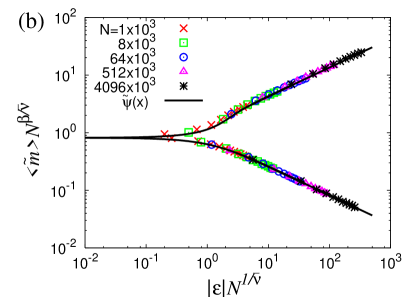
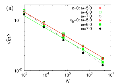
Figure 4: (Color online) Monte Carlo simulation data at $\lambda=6$. (a) The order parameters $\langle\tilde{m}\rangle_{c}$ at $\epsilon=0$ and $\langle\tilde{m}\rangle_{b,c}$ at $\epsilon_{b}=0$ with different values of $(d,\omega)=(2.25,5)$, $(3,6)$, and $(3,7)$ are plotted with symbols. They are compared with the analytic results of Eqs. (24) and (37) which are drawn with lines. Numerical values of the coefficients are $A_{e}\simeq 0.815~{}860$, $\tilde{A}_{e}\simeq 0.687~{}983$, and $B_{e}\simeq 1.039~{}20$. (b) Scaling plot of $\langle\tilde{m}\rangle N^{\beta/\bar{\nu}}$ versus $|\epsilon|N^{1/\bar{\nu}}$ at $\omega=6$ with $\beta=1/2$ and $\bar{\nu}=2$. Data with different values of $N$ fall onto the scaling function $\tilde{\psi}(|\epsilon|N^{1/2})$ drawn with the solid curve.

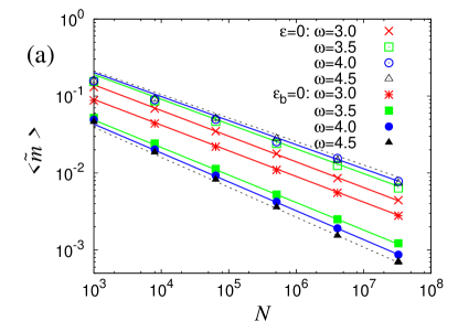
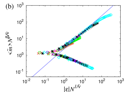
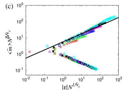
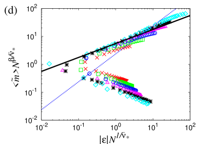
Figure 5: (Color online) Monte Carlo simulation data at $\lambda=4$. The parameter values of $d$ are $2.57$ for $\omega=3$ and $1$ for the other values of $\omega$. (a) Numerical data for $\langle\tilde{m}\rangle_{c}$ and $\langle\tilde{m}\rangle_{b,c}$ represented with symbols are compared with the analytic results represented with straight lines. (b) Scaling plot of $\langle\tilde{m}\rangle N^{1/(\lambda-1)}$ versus $|\epsilon|N^{(\lambda-3)/(\lambda-1)}$ at $\omega=\omega_{\rm nat}=3$. The straight line has the slope of $\beta=1/(\lambda-3)=1$. We also show the scaling collapse of the numerical data at $\omega=4$ according to the FSS forms in (c) Eq. (51) and (d) Eq. (52). The solid line and the dashed line have a slope of $1/2$ and $\beta=1/(\lambda-3)=1$, respectively. We use same symbols of Fig. 4(b) and the symbol $\diamond$ for $N=32~{}768\times 10^{3}$.

We performed extensive Monte Carlo (MC) simulations in the annealed SF networks at various values of $\lambda$ and $\omega$ to confirm the analytic results in Sec. III.2. Especially we focus our attention on the cutoff dependent FSS behavior. In practice, we consider the Ising model on the fully connected network with the heterogeneous coupling constants given by the Hamiltonian in Eq. (8) at all $\tilde{h}_{i}=0$ and set $J=k_{B}=1$.

Using the standard Metropolis single spin update rule, we run MC simulations up to $2\times 10^{3}-10^{4}$ MC steps for system sizes up to $N=32~{}768\times 10^{3}$. The MC data are averaged over 100 independent samples of initial spin configurations as well as the thermal (temporal) average after discarding the data up to $10^{3}$ MC steps for the equilibration.

First, we need to choose a degree sequence $\{k_{i}\}=\{k_{1},\ldots,k_{N}\}$ in accordance with a given degree distribution $P(k)=ck^{-\lambda}$ for $k_{0}\leq k\leq k_{c}$ as in Eq. (28), with $k_{0}=\mathcal{O}(1)$ and $k_{c}={\rm int}[dN^{1/\omega}]$, where ${\rm int}[x]$ denotes the integer part of $x$. Let $N_{k}$ be the number of nodes with degree $k$. Such a degree sequence can be generated deterministically JDNoh2009 by applying the rule

$$\sum_{k^{\prime}=k}^{k_{c}}N_{k^{\prime}}={\rm int}\left[N\sum_{k^{\prime}=k}^{k_{c}}P(k^{\prime})\right]$$ (54)

to $N_{k}$ for all $k$ in the descending order from $k=k_{c}$.

The maximum degree $k^{\prime}_{c}$ thus obtained may be different form the target value $k_{c}$. In fact, $k^{\prime}_{c}$ can be estimated from the condition $N\sum_{k=k^{\prime}_{c}}^{dN^{1/\omega}}P(k)=1$, which yields $k^{\prime}_{c}=dN^{1/\omega}[1+\mathcal{O}(N^{-1+\omega_{\rm nat}/\omega})]$ for $\omega>\omega_{\rm nat}$. Therefore, Eq. (54) indeed yields the degree cutoff scaling with the prescribed values of $d$ and $\omega$ only with a higher-order correction. However, when $\omega=\omega_{\rm nat}$, we find that $k^{\prime}_{c}=d^{\prime}N^{1/\omega}$ with

$$d^{\prime}=d(1+(\lambda-1)d^{\lambda-1}\zeta(\lambda,k_{0}))^{-1/(\lambda-1)}.$$ (55)

When one compares numerical data with the analytic results, the modified value $d^{\prime}$ should be used for $\omega=\omega_{\rm nat}=\lambda-1$. In this section, we use the degree sequences generated deterministically from Eq. (54) for various $N$, $\lambda$, $d$, and $\omega$ with fixed $k_{0}=3$.

Monte Carlo simulation data for $\lambda=6$ are presented in Fig. 4. We first test whether the magnetizations $\langle\tilde{m}\rangle_{c}$ at the pseudo critical temperature with $\epsilon=0$ and $\langle\tilde{m}\rangle_{b,c}$ at the bulk critical temperature with $\epsilon_{b}=0$ scale as in Eqs. (24) and (37), respectively. In order to cover the three cases of Eq. (37), we choose $\omega=5$, $6$, and $7$, which correspond to $\alpha=3/5$, $1/2$, and $3/7$, respectively. These numerical data in Fig. 4(a) are in good agreement with the analytic results.

Our analytic theory predicts the full shape of the scaling function as well as the scaling exponents. We examine validity of the FSS form in Eq. (60) in Fig. 4(b). We present the scaling plot of $\langle\tilde{m}(\epsilon,N)\rangle$ against $|\epsilon|N^{1/\bar{\nu}}$ using the Monte Carlo data with $\lambda=6$ and $\omega=6$. These data match perfectly well with the analytic curve for the scaling function $\tilde{\psi}(|\epsilon|N^{1/2})$ in Eq. (61).

We proceed to the case with $\lambda=4$, where the FSS behavior is more complicated. We first examine the FSS of $\langle\tilde{m}\rangle_{c}$ at $\epsilon=0$ and $\langle\tilde{m}\rangle_{b,c}$ at $\epsilon_{b}=0$. They are predicted to follow the power law given in Eqs. (46) and (53), respectively, when $\omega>\omega_{\rm nat}$. When $\omega=\omega_{\rm nat}$, the scaling is given by the same power law but with modified amplitudes. Figure 5(a) presents the plots of $\langle\tilde{m}\rangle_{c}$ and $\langle\tilde{m}\rangle_{b,c}$ against $N$ at $\omega=3$, $3.5$, $4$, and $4.5$, which agree well with the theoretical curves.

When $\omega=\omega_{\rm nat}$, the FSS is governed with the single scaling variable $\epsilon N^{(\lambda-3)/(\lambda-1)}$. In Fig. 5(b), we present the scaling plot of $\langle\tilde{m}\rangle N^{1/(\lambda-1)}$ against $|\epsilon|N^{(\lambda-3)/(\lambda-1)}$ at $\lambda=4$ and $\omega=3$. A good data collapse supports that FSS form with the single scaling variable. We note that the bulk scaling behavior $\langle\tilde{m}\rangle\sim\epsilon^{\beta}$ with $\beta=1/(\lambda-3)$ sets in only for $N\gg 10^{6}$.

We also examine the FSS behavior at $\omega=4~{}(>\omega_{\rm nat})$. Here, the FSS is governed with two scaling variables $\epsilon N^{1/\bar{\nu}_{c}}$ and $\epsilon N^{1/\bar{\nu}_{*}}$. Hence, one cannot expect a data collapse over the whole regions in a scaling plot. We first test the scaling form of Eq. (51), which is valid in regimes II, III, and IV. The scaling plot of $\langle\tilde{m}\rangle N^{\tilde{\beta}/\bar{\nu}_{c}}$ against the scaling variable $|\epsilon|N^{1/\bar{\nu}_{c}}$ is presented in Fig. 5(c). We observe a reasonably good data collapse in regimes II, III, and IV except for small network sizes. In the $\epsilon>0$ side, the numerical data align along a straight line of slope $1/2$, which reflects the scaling $\langle\tilde{m}\rangle\sim\epsilon^{1/2}$ in regime II. However, they begin to deviate from the straight line systematically for $N\geq 4096\times 10^{3}$ as the scaling variable increases. This is due to the crossover to regime I.

Finally, we test the scaling form of Eq. (52), which is valid in regimes I and II. Figure 5(d) shows the scaling plot of $\langle\tilde{m}\rangle N^{\beta/\bar{\nu}_{*}}$ against the scaling variable $|\epsilon|N^{1/\bar{\nu}_{*}}$. As expected, we do not have a data collapse for $\epsilon\leq 0$. The data in regimes I and II do not collapse well either. The order parameter scales as $\langle\tilde{m}\rangle\sim\epsilon^{1/2}$ in regime I and then $\langle\tilde{m}\rangle\sim\epsilon^{1/(\lambda-1)}=\epsilon^{1}$ in regime II. Comparing the numerical data with the straight lines of slopes of $1/2$ and $1$, one finds the signature of the crossover for $N\geq 4096\times 10^{3}$. This suggests that the poor data collapse may be due to a finite size effect. The system does not reach the scaling regime I even at $N=32~{}768\times 10^{3}$ yet.

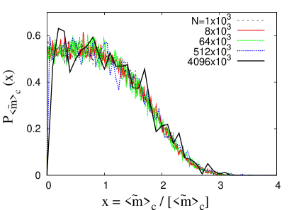
Figure 6: (Color online) The histogram for $\langle\tilde{m}\rangle_{c}/[\langle\tilde{m}\rangle_{c}]$, the order parameter at $\epsilon=0$ normalized with the ensemble average, where network parameters are $\lambda=4.0$, $k_{0}=3$, $d=1$, and $\omega=\omega_{\rm nat}=3$. The curves from different values of $N$ collapse onto a single curve.

V Sample-to-Sample Fluctuations

In the previous section, we tested the FSS theory for the power-law degree distributions generated deterministically from Eq. (54). The other way is to draw probabilistically $N$ values of the degree independently in accordance with the target distribution function $P(k)$. This is adopted in the configuration model Newman2001 ; CBP-S2005 . In the probabilistic method, the degree sequence varies from sample to sample, hence an ensemble average is necessary. One interesting issue is whether physical quantities have the self-averaging property Aharony1996 against the sample-to-sample fluctuations. For finite systems, a sample with $\{k_{i}\}=\{k_{1},\ldots,k_{N}\}$ drawn probabilistically may show the degree distribution $\tilde{P}(k)=\sum_{i}\delta_{k,k_{i}}/N$, which deviates from the target distribution function $P(k)$. Then, it follows that the degree moments $z_{n}=\sum_{i}k_{i}^{n}/N$ show the sample-to-sample fluctuations, purely from the sampling disorder.

Using the same techniques used in our previous publication for the CP model JDNoh2009 (see Sec. V therein), it is straightforward to show that the relative fluctuation $R_{n}$ is given by

$$R_{n}\equiv\frac{[z_{n}^{2}]-[z_{n}]^{2}}{[z_{n}]^{2}}=\frac{1}{N}\left(\frac{\langle 2n\rangle_{0}}{\langle n\rangle_{0}^{2}}-1\right),$$ (56)

where $[\cdots]$ denotes the sample (disorder) average and $\langle n\rangle_{0}\equiv\sum_{k}k^{n}P(k)$. For exponential networks, all $\langle n\rangle_{0}$ are finite, so all degree moments $z_{n}$ are strongly self-averaging ($R_{n}\sim N^{-1}$) Aharony1996 .

In the SF networks with $P(k)$ given in Eq. (28),

$$\langle n\rangle_{0}\sim\left\{\begin{array}[]{lll}N^{(n-\lambda+1)/\omega}&\mbox{for}&n>\lambda-1\\[5.69054pt] \log N&\mbox{for}&n=\lambda-1\\[5.69054pt] \mathcal{O}(1)&\mbox{for}&n<\lambda-1,\end{array}\right.$$ (57)

which leads to

$$R_{n}\sim\left\{\begin{array}[]{lll}N^{-1+(\lambda-1)/\omega}&\mbox{for}&n>\lambda-1\\[5.69054pt] N^{-1+(2n-\lambda+1)/\omega}&\mbox{for}&(\lambda-1)/2<n<\lambda-1\\[5.69054pt] N^{-1}&\mbox{for}&n<(\lambda-1)/2,\end{array}\right.$$ (58)

where there are log corrections at $n=\lambda-1$ and $(\lambda-1)/2$. By definition, $R_{n}$ is strongly self-averaging for $n<(\lambda-1)/2$ and is weakly self-averaging for $n>(\lambda-1)/2$ except that $R_{n}$ is not self-averaging only when $\omega=\omega_{\rm nat}$ for $n>\lambda-1$. For example, $z_{4}$ is not self-averaging for $\lambda<5$ with the natural upper cutoff.

The relevant quantities involving the degree moments are $\tilde{K}_{c}=z_{1}/z_{2}$, $a=z_{1}^{2}/z_{2}$, and $b=(z_{1}/z_{2})^{4}z_{4}$. It implies that the critical point location and $a$ are strongly self-averaging for $\lambda>5$ and at least weakly self-averaging for $\lambda>3$. However, $b$ is not self-averaging for $3<\lambda<5$ with $\omega=\omega_{\rm nat}$, which determines the amplitude of the order parameter in various scaling regimes [see Eqs. (46) and (48)]. Therefore, we expect widely scattered data for the order parameter, depending strongly on sampled degree sequences, for $3<\lambda<5$ with $\omega=\omega_{\rm nat}$.

Numerical data are presented to verify the non-self-averaging property of the order parameter at $\epsilon=0$, $\langle\tilde{m}\rangle_{c}\sim(bN)^{-1/4}$ [see Eq. (46)], for the annealed SF networks for $\lambda=4$ with $\omega=\omega_{\rm nat}=3$. It should not be self-averaging because it involves the parameter $b$. We have measured the order parameter $\langle\tilde{m}\rangle_{c}$ in many samples and constructed a histogram of the quantity $\langle\tilde{m}\rangle_{c}/[\langle\tilde{m}\rangle_{c}]$, the order parameter normalized with its mean values.

Figure 6 presents, thus, the obtained histogram. The histogram does not sharpen at all, but collapses onto a single curve as $N$ increases. This proves the non-self-averaging property.

VI Summary and discussion

We have investigated the FSS of the Ising model on annealed networks. The model is mapped to the Ising model on a globally connected network with heterogeneous couplings, which allows us to derive the free-energy density as a function of the magnetic order parameter $\tilde{m}$. Using the free energy density function, the scaling functions for $\tilde{m}$ and the zero-field susceptibility $\tilde{\chi}$ are also derived.

For the networks with exponentially bounded degree distributions and power-law degree distributions with $\lambda>5$, the FSS forms are given in Eqs. (60) and (62). The critical exponents for the magnetization and the susceptibility are given by $\beta=1/2$ and $\gamma=1$, respectively. The FSS exponent is given by $\bar{\nu}=2$, with which the scaling variable for the FSS is given by $\epsilon N^{1/\bar{\nu}}$. The scaling behaviors in the critical regime [$\epsilon N^{1/\bar{\nu}}=\mathcal{O}(1)$], in the supercritical regime ($\epsilon\gg N^{-1/\bar{\nu}}$), and in the subcritical regime ($\epsilon\ll-N^{-1/\bar{\nu}}$) are summarized in Figs. 1 and 2.

For power-law degree distributions with $3<\lambda<5$, the degree cutoff $k_{c}\sim N^{1/\omega}$ matters and there exist two distinct scaling variables $\epsilon N^{1/\bar{\nu}_{c}}$ with $\bar{\nu}_{c}=2/[1-(5-\lambda)/\omega]$ and $\epsilon N^{1/\bar{\nu}_{*}}$ with $\bar{\nu}_{*}=\omega/(\lambda-3)$ when $\omega>\omega_{\rm nat}=\lambda-1$. At $\omega=\omega_{\rm nat}$, the two scaling variables merge into a single one. The scaling behaviors in the supercritical regime I ($\epsilon\gg N^{-1/\bar{\nu}_{*}}$), the intermediate regime II ($N^{-1/\bar{\nu}_{c}}\ll\epsilon\ll N^{-1/\bar{\nu}_{*}}$), the critical regime III [$\epsilon N^{1/\bar{\nu}_{c}}=\mathcal{O}(1)$], and the subcritical regime IV ($\epsilon\ll-N^{1/\bar{\nu}_{c}}$) are summarized in Fig. 3. The crossover from regime I to II is originated from the finiteness of the degree cutoff $k_{c}$, while the critical FSS in regime III is from the finiteness of both $k_{c}$ and $N$.

The CP on the annealed SF network studied in Refs. Boguna2009 ; JDNoh2009 is also characterized with the two $\omega$-dependent FSS exponents when $2<\lambda<3$ and $\omega>\omega_{\rm nat}$. The similarity between the equilibrium Ising model and the nonequilibrium CP suggests that the two-parameter scaling is a generic feature of critical phenomena in annealed scale-free networks.

Extensive studies during the last decade have revealed that critical phenomena on quenched networks and annealed networks are characterized with the same set of bulk critical exponents such as the order parameter exponent and susceptibility exponent. However, they display distinct FSS behaviors. Annealed networks are characterized with two FSS exponents, which depend on $\lambda$ and $\omega$. In comparison to annealed networks, quenched networks have a quenched disorder in structure. Besides, dynamic degrees of freedom on quenched networks have finite correlations. It is another big challenge to understand how these two ingredients cause the distinct FSS behaviors, some of which is under investigation FSS-full .

Appendix A scaling functions

From the free energy density function in Eq. (19) for the exponential networks and also the SF networks with $\lambda>5$, one can easily derive $\langle\tilde{m}\rangle$ for small $\tilde{h}$ as

$$\langle\tilde{m}\rangle\simeq\left(\frac{12}{bN}\right)^{1/4}\frac{U(1/2,r)+a^{\prime}N^{3/4}\tilde{h}U(3/4,r)}{U(1/4,r)+a^{\prime}N^{3/4}\tilde{h}U(1/2,r)},$$ (59)

where $a^{\prime}=(12/b)^{1/4}a$, $r=(3a^{2}/b)^{1/2}\epsilon N^{1/2}$, and

$$U(s,r)=\int_{0}^{\infty}dy\ y^{s-1}\exp(-y+r\sqrt{y}).$$

With this, we find the order parameter scaling at $\tilde{h}=0$ as

$$\langle\tilde{m}(\epsilon,N)\rangle=N^{-\beta/\bar{\nu}}\tilde{\psi}(\epsilon N^{1/\bar{\nu}};a,b),$$ (60)

where $\beta=1/2$, $\bar{\nu}=2$, and

$$\tilde{\psi}(x;a,b)=\left(\frac{12}{b}\right)^{1/4}\frac{U(1/2,r_{0}x)}{U(1/4,r_{0}x)},$$ (61)

with $r_{0}=(3a^{2}/b)^{1/2}$ and $x=\epsilon N^{1/\bar{\nu}}$.

The zero-field susceptibility $\tilde{\chi}=(\partial\langle\tilde{m}\rangle)/(\partial\tilde{h})|_{\tilde{h}=0}$ is

$$\tilde{\chi}(\epsilon,N)=N^{\gamma/\bar{\nu}}\tilde{\phi}(\epsilon N^{1/\bar{\nu}};a,b),$$ (62)

where $\gamma=1$ and

$$\tilde{\phi}(x;a,b)=a\left(\frac{12}{b}\right)^{1/2}\left[\frac{U(3/4,r_{0}x)}{U(1/4,r_{0}x)}-\frac{U^{2}(1/2,r_{0}x)}{U^{2}(1/4,r_{0}x)}\right].$$ (63)

Using the properties of the function $U(s,r)$ such as

$$U(s,r)\simeq\left\{\begin{array}[]{ll}2\Gamma(2s)\ (-r)^{-2s}&(r\rightarrow-\infty)\\[5.69054pt] \Gamma(s)&(r=0)\\[5.69054pt] 2\pi^{\frac{1}{2}}e^{\frac{r^{2}}{4}}\left(\frac{r}{2}\right)^{2s-1}\left[1+\frac{4(s-1)(s-2)}{r^{2}}\right]&(r\rightarrow\infty),\end{array}\right.$$ (64)

one can show $\tilde{\psi}(x)\simeq\sqrt{3a/b}\ x^{1/2}$ or $\sqrt{2/(\pi a)}(-x)^{-1/2}$ for $x\rightarrow\pm\infty$, and $\tilde{\phi}(x)\simeq(2x)^{-1}$ or $(1-2/\pi)(-x)^{-1}$ for $x\rightarrow\pm\infty$. We remark that the usual magnetization and the magnetic susceptibility become $m\simeq a\langle\tilde{m}\rangle$ and ${\chi}\simeq a\tilde{\chi}$.

For the SF networks with $3<\lambda<5$, the scaling function $\tilde{\psi}_{c}(x)$ for the order parameter near $\epsilon\approx 0$ in Eq. (51) behaves in the same way as the above $\tilde{\psi}(x)$ except for replacing $\beta$ by $\tilde{\beta}$, $\bar{\nu}$ by $\bar{\nu}_{c}$, and $b$ by $b_{0}$. For example, $r$ becomes $r=(3a^{2}/b_{0})^{1/2}\epsilon N^{1/\bar{\nu}_{c}}$. The susceptibility scaling function also changes in the same way.

References

• (1) M. E. J. Newman, SIAM Rev. 45, 167 (2003); R. Albert and A.-L. Barabási, Rev. Mod. Phys. 74, 47 (2002); S. N. Dorogovtsev and J. F. F. Mendes, Adv. Phys. 51, 1079 (2002); S. Boccaletti, V. Latora, Y. Moreno, M. Chavez, and D.-U. Hwang, Phys. Rep. 424, 175 (2006).
• (2) S. N. Dorogovtsev and J. F. F. Mendes, Evolution of Networks: From Biological Nets to the Internet and WWW (Oxford University Press, Oxford, 2003).
• (3) S. N. Dorogovtsev, A. V. Goltsev, and J. F. F. Mendes, Rev. Mod. Phys. 80, 1275 (2008).
• (4) For a review, see Finite-Size Scaling and Numerical Simulation of Statistical Systems, ed. by V. Privman (World Scientific, Singapore, 1990).
• (5) H. Hong, M. Ha, and H. Park, Phys. Rev. Lett. 98, 258701 (2007).
• (6) M. Ha, H. Hong, and H. Park, Phys. Rev. Lett. 98, 029801 (2007).
• (7) C. Castellano, and R. Pastor-Satorras, Phys. Rev. Lett. 98, 029802 (2007).
• (8) C. Castellano and R. Pastor-Satorras, Phys. Rev. Lett. 100, 148701 (2008).
• (9) M. Boguñá, C. Castellano, and R. Pastor-Satorras, Phys. Rev. E 79, 036110 (2009).
• (10) J. D. Noh and H. Park, Phys. Rev. E 79, 056115 (2009).
• (11) M. E. J. Newman, S. H. Strogatz, and D. J. Watts, Phys. Rev. E 64, 026118 (2001).
• (12) M. Catanzaro, M. Boguñá, and R. Pastor-Satorras, Phys. Rev. E 71, 027103 (2005).
• (13) J. Park and M. E. J. Newman, Phys. Rev. E 70, 066117 (2004).
• (14) The maximum value of pijN2/ω1similar-tosubscript𝑝𝑖𝑗superscript𝑁2𝜔1p_{ij}\sim N^{2/\omega-1} with kcN1/ωsimilar-tosubscript𝑘𝑐superscript𝑁1𝜔k_{c}\sim N^{1/\omega} and ωλ1𝜔𝜆1\omega\geq\lambda-1 in the SF networks with P(k)kλsimilar-to𝑃𝑘superscript𝑘𝜆P(k)\sim k^{-\lambda}. Therefore, the condition that pij1much-less-thansubscript𝑝𝑖𝑗1p_{ij}\ll 1 for large N𝑁N is valid for general ω𝜔\omega only when λ>3𝜆3\lambda>3.
• (15) G. Bianconi, Phys. Lett. A 303, 166 (2002).
• (16) F. Iglói and L. Turban, Phys. Rev. E 66, 036140 (2002).
• (17) A. V. Goltsev, S. N. Dorogovtsev, and J. F. F. Mendes, Phys. Rev. E 67, 096123 (2003).
• (18) F. Caccioli and L. Dall’Asta, J. Stat. Mech.: Theory Exp. 2009 P10004.
• (19) E. Elizalde, S. D. Odintsov, A. Romeo, A. A. Bytsenko, and S. Zerbini, Zeta Regularization Techniques with Applications (World Scientific, Singapore, 1994).
• (20) A. Aharony and A.B. Harris, Phys. Rev. Lett. 77, 3700 (1996).
• (21) M. Ha, H. Hong, and H. Park (unpublished).