Independence and interdependence in the nest-site choice by honeybee swarms:
agent-based models, analytical approaches and pattern formation

Abstract

In a recent paper List, Elsholtz and Seeley List et al. (2009) have devised an agent-based model of the the nest-choice dynamics in swarms of honeybees, and have concluded that both interdependence and independence are needed for the bees to reach a consensus on the best nest site. We here present a simplified version of the model which can be treated analytically with the tools of statistical physics and which largely has the same features as the original dynamics. Based on our analytical approaches it is possible to characterize the co-ordination outcome exactly on the deterministic level, and to a good approximation if stochastic effects are taken into account, reducing the need for computer simulations on the agent-based level. In the second part of the paper we present a spatial extension, and show that transient non-trivial patterns emerge, before consensus is reached. Approaches in terms of Langevin equations for continuous field variables are discussed.

I Introduction

In a recent paper List et al. (2009) List, Elsholtz and Seeley (LES for short from now on) presented an agent-based model of the decision making processes in the nest-site choice of honeybee swarms, and their paper has attracted a significant amount of attention in the public media (see e.g. The Economist of 13 February 2009). LES focus on the interplay between the interdependence among bees and their independence in assessing the quality of potential nest sites, and conclude that, assuming a degree of independence, bees will generally choose the best nest site for a wide range of non-extremal model parameters, and secondly that both independence and interdependence are necessary for the swarm to reach a reliable consensus on the best possible nest site. The precise notions of ‘independence’ and ‘interdependence’ will become clear below, but in essence LES find that, in order to identify the best nest site, the bees in their model need to make independent assessments of the true quality of nest sites instead of blindly following the choices advertised by fellow bees. At the same time interdependence, i.e. direct communication between bees, is required as well in order to promote a quick and accurate convergence towards a consensus on the best choice.

While the work of LES is mainly based on computer simulations, we here discuss a modification of their agent-based dynamics, which can be addressed using the tools and techniques of statistical mechanics. Such analytical solutions mean that computer simulations on the agent-based level could in principle be dispensed with entirely, although admittedly our resulting equations still require numerical solution. Still, if there are $k$ nest sites in the model, then on the deterministic level, the solution of the reduced model comes out as a coupled set of $k$ quadratic equations for the number of bees advertising the different sites, which is a significant reduction in complexity of the problem. LES choose $k=5$ in their analysis, so that we are able to reduce the deterministic features of their model to a very small set of equations. Of course, stochasticity is important in the model, but given the deterministic solution, fluctuations about the deterministic limit can be characterized analytically as well to a good approximation, as we will describe below. The main aim of this current paper is to present the modified version of LES’s model, and to show how it can be addressed with the tools of statistical physics. In the second part of our work we then extend the model of List et al. (2009) to include space, and study the pattern formation dynamics of this extended model.

The natural process modeled by LES is the following: once a year once a colony of bees has reached a certain size, a ‘search committee’ consisting of several hundred bees swarm out to identify suitable nest sites, and once an agreement has been reached the original colony divides, and the queen leaves with about two thirds of the bees for the new nest (see List et al. (2009) and references therein). The process LES are interested in is the actual decision making. The bees who fly out to inspect potential new sites return to the original colony and perform dances to advertise the new sites they have inspected. The duration of the dance here is a measure for the quality of a newly inspected site, the better the site, the longer the dance. Fellow bees who observe these dances might then themselves start dancing for that particular site as well, and this may happen with or without an independent inspection of the actual site, i.e. with or without an independent assessment of the site’s quality. This may then lead to other bees initiating dances (again with or without independent assessment of the site’s quality), and finally, if all goes well, a general consensus on one of the nest sites will be reached. The question LES address in their model is whether this consensus will be on the best possible site, or whether a sub-optimal choice can result.

In order to model communication and interdependence between bees LES assume that the rate with which a given bee starts dancing for a particular site depends on an a-priori rate of independently discovering that site, and, weighted by an ‘interdependence coefficient’, the fraction of other bees dancing for this site. If the interdependence between bees is strong then the latter factor carries a large weight, and the rate with which bees start dancing for a given site is mostly determined by the fraction of bees already dancing for that site. If interdependence is weak dances for all sites are commenced essentially with equal rates, independently of how many bees are already advertising the different sites. The second component of the model is the time a dance lasts once it has been begun. In the model by LES, the duration of the dance is determined by a combination of the actual (or perceived) quality of the site, and a uniform site-independent contribution. In the case of strong independence, the bees are assumed to inspect the site before dancing for it, and the duration of the dance will be proportional to the perceived quality of the site. In the case of weak independent quality assessment the duration of the dance for a given site does not depend much on the site’s quality.

The key question LES address in their study is whether or not the swarm of bees will eventually reach a consensus on what the best nest-site might be, and whether this consensus choice then is the actual best site. The outcome of the decision dynamics here depends on the independence and interdependence parameters introduced above, and, to a lesser extent, on the accuracy with which bees assess the quality of a site if they actually inspect it. I.e. a bee may decide to visit a site before dancing for it, but the perceived quality may be a random function of the actual quality, so that noise may blur the bee’s assessment of the site. In this paper we complement the simulation study of LES by analytical computations, allowing for a more extensive characterization of the model. We also present extensions towards a spatial model, and discuss how patterns may emerge at transient times if the model is considered on a two-dimensional regular lattice. The paper is organized as follows: In Sec. II we will first re-iterate the definitions of the model by LES, and then introduce the simplified dynamics, which we will then address analytically within a master equation approach in Sec. III. We here formulate deterministic mean-field equations and also address first-order finite-size corrections. In Sec. IV we then introduce a spatial version of the reduced model, and show in computer simulations that non-trivial transient patterns may emerge if model parameters are chosen suitably. The study of the spatial model is complemented by the numerical integration of a set of partial differential equations for a coarse-grained dynamics. In Sec. V we finally summarize our work and point to future directions which may be of interest.

II Model definitions

II.1 Original model by List et al

In the original model by LES there are $N$ bees, labelled $i=1,2,\dots,N$, and $k$ potential nest sites, we label them by $\alpha=1,\dots,k$. Each nest site has an intrinsic quality $q_{\alpha}\geq 0$. These ‘actual’ qualities of the different nest sites are fixed from the beginning and do not change over time. We always choose $q_{1}<q_{2}<\dots<q_{k}$, i.e. site number $k$ is the best site, and site number $1$ the worst. Additionally, for each potential nest site $\alpha$, there is an a-priori probability $\pi_{\alpha}$ of finding this particular site. These rates of finding the different nests will be taken to fulfill $\sum_{\alpha=1}^{k}\pi_{\alpha}<1$, and we will set $\pi_{0}=1-\sum_{\alpha=1}^{k}\pi_{\alpha}$. Throughout this paper we will follow List et al. (2009) and assume that the $\pi_{\alpha}$, $\alpha=1,\dots,k$, are identical for all nests, but an extension of the model to the more general case is straightforward.

The decision and dancing dynamics within the model then proceeds in discrete time steps, $t=1,2,3,\dots$, and at each time step each bee can either be dancing for a particular site $\alpha\in\{1,\dots,k\}$, or not be dancing. The not-dancing state here describes bees that may have flown out to inspect a site, but have not yet started dancing for it, as well as bees who are observing other bees, or bees that are resting List et al. (2009). We will sometimes refer to these bees as ‘passive’. Following LES we write $s_{i}(t)=\alpha\in\{1,\dots,k\}$ if bee number $i$ is dancing for site $\alpha$ at time $t$, and $s_{i}(t)=0$, if she is not dancing at time $t$. In LES’s model, the state of a bee is characterized by an additional variable, $d_{i}(t)\geq 0$, indicating the remaining duration of bee $i$’s dance at time $t$. I.e., up to rounding to a near integer, if $d_{i}(t)\geq 1$, then bee $i$ will be dancing for another $d_{i}(t)$ time steps. In the non-dancing state (i.e. for a bee $i$ with $s_{i}(t)=0$) $d_{i}(t)$ has no relevance. More specifically, the dynamics proceeds according to the following algorithm:

1. At time $t=0$ initialize the $\{s_{i}(t),d_{i}(t)\}$, for example set $s_{i}(t=0)=0$, and $d_{i}(t)=0$ for all $i$.

2. At time $t$ compute the fraction of passive bees and of those dancing for the different sites $\{\alpha\}$ at this time, $f_{\alpha}(t)=N^{-1}\sum_{i=1}^{N}\delta_{\alpha,s_{i}(t)}\in[0,1]$ ($\alpha=0,\dots,k$). $\delta$ here stands for the Kronecker delta, i.e. $\delta_{\alpha\beta}=1$ if $\alpha=\beta$, and $\delta_{\alpha\beta}=0$ otherwise. Then compute $p_{\alpha}(t+1)=(1-\lambda)\pi_{\alpha}+\lambda f_{\alpha}(t)$ ($\alpha=0,\dots,k$). Note that $\sum_{\alpha=0}^{k}p_{\alpha}(t+1)=1$ by construction, due to the normalization of the $\pi_{\alpha}$ and of the $f_{\alpha}$. The variable $\lambda\in[0,1]$ is a model parameter, and its meaning will be explained below.

3. In order to update the states of the bees distinguish between bees that are not dancing at time $t$ and those which are dancing at time $t$. Update all bees in parallel dynamics, i.e. for all $i=1,\dots,N$ perform the following:

   • If bee $i$ is dancing at time $t$, then check whether $d_{i}(t)\geq 1$. If this is the case then the bee keeps dancing for the site she is currently dancing for, i.e. set $s_{i}(t+1)=s_{i}(t)$ and reduce the remaining duration of the dance by one unit: $d_{i}(t+1)=d_{i}(t)-1$. If the bee is dancing, but $d_{i}(t)<1$, then set $s_{i}(t+1)=0$ and $d_{i}(t+1)=0$ (the bee stops dancing).

   • If, at time $t$, bee $i$ is not dancing ($s_{i}(t)=0$), then with probability $p_{\alpha}(t+1)$ set $s_{i}(t+1)=\alpha$ ($\alpha=1,\dots,k$), i.e. with probability $p_{1}(t+1)$ the bee starts dancing for site $\alpha=1$, with probability $p_{2}(t+1)$ she starts dancing for site $\alpha=2$ and so on. With probability $p_{0}(t+1)$ she will remain in the non-dancing state. If a dance is commenced then it remains to specify the duration of the dance bee $i$ has just started for site $\alpha$. Here draw a random number $T$ from a standard Gaussian distribution (mean zero, unit variance). Then set

     $$~{}~{}~{}~{}~{}~{}~{}~{}~{}~{}~{}~{}~{}~{}~{}~{}~{}~{}~{}~{}~{}d_{i}(t+1)=\left\{\begin{array}[]{cl}q_{\alpha}\exp(\sigma T)&~{}\mbox{with prob. }1-\mu\\ {}\hfil&{}\\ K\exp(\sigma T)&~{}\mbox{with prob. }\mu\end{array}\right.$$

4. Iterate, i.e. go to 2.

LES here set $K=q_{k}$, i.e. $K$ is the quality of the best site. The variables $\lambda\in[0,1]$ and $1-\mu\in[0,1]$ are the interdependence and independence parameters mentioned in the introduction. If $\lambda$ is close to one, then the interdependence between bees is strong, i.e. the rate of commencing a dance for a given site is mostly determined by the number of bees already dancing for this site. At small $\lambda$ the dancing activity of other bees is mostly irrelevant for a given individual to take up a dance. The independence in the assessment of the nest-site qualities is parametrized by $\mu$, more accurately by $1-\mu$ in the notation of LES which we will follow here. For large $1-\mu$ the duration of a dance for site $\alpha$ strongly depends on the quality $q_{\alpha}$ of that site (independent assessment), whereas for small $1-\mu$, the actual quality of the different sites is mostly irrelevant for the duration of the dances. The variable $\sigma\geq 0$ is a further model parameter and represents the reliability of the bees’ assessment of the qualities of the different sites. As seen in the above update rules the perceived quality of site $\alpha$ is given by $q_{\alpha}\exp(\sigma T)$, where $T$ is a standard Gaussian random variable. Thus if $\sigma=0$, the perceived quality is always identical to the actual quality $q_{\alpha}$. Increasing $\sigma$ introduces more and more uncertainty into this perception.

The dynamics as defined above is easily implemented in a computer simulation, and LES have presented an extensive numerical analysis of the model. For completeness we present some simulation results in Fig. 1, where we show the fraction of bees dancing for the different sites in a situation where there are five potential nest-sites, and with strong independence ($1-\mu=1$), and varying interdependence. As seen in the figure, the best nest-site tends to be the most populated one on average, but convergence to the best nest-site is strong only at moderate to high interdependence, but not so much at low values of $\lambda$.

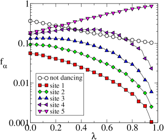
Figure 1: Original model by List et al: Fraction $f_{\alpha}$ of bees dancing for each of the sites, $\alpha=1,2\dots,5$, in the stationary state, along with the fraction of bees who are not dancing, $f_{0}$, versus $\lambda$ at fixed $\mu=0$. Markers from simulations ($N=200$, run for $1000$ steps, averaged over $10$ runs). Model parameters are $k=5$, $(q_{0},q_{1},q_{2},q_{3},q_{4},q_{5})=(0.1,3,5,7,9,10)$, $\sigma=0.2$, and $\pi_{\alpha}=0.05$ for all $\alpha=1,\dots,5$.

II.2 Simplified model

If one introduces state variables $x_{i}(t)=(s_{i}(t),d_{i}(t))$, as LES do, then the above dynamics defines a Markov chain in the state space spanned by the $\{x_{i}\}$, $i=1,\dots,N$, and a master equation approach is feasible in principle. However, as we will discuss in the next section, the model can actually be reduced first, without affecting its key features and behavior much, to yield a dynamics which is Markovian in the space of the $\{s_{i}(t)\}$ alone. This simplifies the analysis considerably, and as we will show next, the ‘memory’ variables $d_{i}(t)$ can be dispensed with entirely.

The simplified model operates purely in the space of the $\{s_{i}(t)\}$, i.e. the state of the system at any given time is fully determined by the variables $s_{1}(t),\dots,s_{N}(t)$. In essence the simplification consists in the following step: if in the original model a bee begins to dance for a given site at a given time $t$, the duration $d_{i}(t)$ of this dance is determined at the beginning of the dance, and then, up to rounding to a near integer, at time step $t+d_{i}(t)$ the bee stops dancing for this given site. For $\mu<1$, the duration of the dance depends on the quality of the site danced for, and is also subject to some uncertainty as explained above. But crucially, the duration of the dance is set at the beginning of the dance, the end of the dance then occurs at a deterministic moment in time, once the duration has been chosen. The duration of the dance may have a stochastic element to it as explained above, but its value is fixed and known when the dance starts. In the reduced model we replace this with a random process, i.e. a bee may start dancing for a given site $\alpha$ at time $t$, and then at each subsequent time step the bee ceases dancing with a certain probability $r_{\alpha}$ and continues dancing with probability $1-r_{\alpha}$. The rate $r_{\alpha}$ with which the dance is stopped at each step may here depend on the quality of the site, for example a high-quality site $\alpha$ will have a lower value of $r_{\alpha}$ than a site $\beta$ of a lesser quality. The probability that a dance for a given site $\alpha$ lasts for precisely $\ell$ time-steps after the dance has begun is then given by $(1-r_{\alpha})^{\ell-1}r_{\alpha}$, i.e. it follows a geometric distribution of mean $1/r_{\alpha}$. This may be slightly unrealistic in the sense that the probability of stopping after exactly $\ell$ rounds is a monotonically decreasing function of $\ell$, whereas the distribution of dance durations used by LES has a well-defined maximum, but this drawback is, in our view, largely outweighed by the analytical simplifications it brings with it. As we will show below this simplification does not affect the qualitative behavior of the model much. A further restriction of the reduced model is the fact that there is no clear analogue of the uncertainty parameter $\sigma$ in the present setup, i.e. once $r_{\alpha}$ has been chosen, both the mean and variance of the distribution of durations of dances for site $\alpha$ are fixed. We will discuss possibilities to include such uncertainty towards the end of this paper.

The precise algorithm of the simplified model is the following, the definitions and conventions regarding the $\{\pi_{\alpha}\}$ and the model parameters $\lambda$ and $\mu$ are the same as in the original model:

1. At time $t=0$ initialize the $\{s_{i}(t=0)\}$ for all $i$, for example set all bees in a non-dancing state, or initialize the $s_{i}(t)$ at random.

2. At time $t$ compute the fraction $f_{\alpha}(t)\in[0,1]$ of bees dancing for site $\alpha$ at time $t$ ($\alpha=0,\dots,k$), and compute $p_{\alpha}(t+1)=(1-\lambda)\pi_{\alpha}+\lambda f_{\alpha}(t)$. Note that $0\leq p_{\alpha}(t+1)\leq 1$ for all $\alpha$, and $\sum_{\alpha=0}^{k}p_{\alpha}(t+1)=1$ by definition.

3. In order to update the states of the bees distinguish between bees that are not dancing at time $t$ and those which are dancing at time $t$. Update all bees in parallel dynamics, i.e. for all $i=1,\dots,N$ perform the following:

   • If bee $i$ is dancing for site $\alpha$ at time $t$ (i.e. if $s_{i}(t)=\alpha>0$), then with probability $r_{\alpha}$ set $s_{i}(t+1)=0$ (bee stops dancing), and with probability $1-r_{\alpha}$ set $s_{i}(t+1)=\alpha$ (bee keeps dancing for site $\alpha$).

   • If, at time $t$, bee $i$ is not dancing ($s_{i}(t)=0$), then with probability $p_{\alpha}(t+1)$ set $s_{i}(t+1)=\alpha$, $\alpha=0,1,\dots,k$, i.e. with probability $p_{1}(t+1)$ the bee starts dancing for site $\alpha=1$, with probability $p_{2}(t+1)$ she starts dancing for site $\alpha=2$ and so on. With probability $p_{0}(t+1)$ she will remain in the passive state $\alpha=0$.

4. Iterate, i.e. go to 2.

It remains to specify the rates with which dances are terminated, i.e. to define the $\{r_{\alpha}\}$. We here choose

$$r_{\alpha}=q_{0}\left[\frac{\mu}{K}+\frac{1-\mu}{q_{\alpha}}\right],~{}~{}~{}~{}\alpha=1,\dots,k,$$ (1)

where $K=q_{k}$ as in List et al. (2009). For any $\mu<1$ the rate $r_{\alpha}$ is a decreasing function of $q_{\alpha}$, i.e. the higher a site’s quality, the lower the rate at which dances for it are stopped. The pre-factor $q_{0}$ (which needs to be non-zero) here ensures that $0<r_{\alpha}\leq 1$ and also that the $\{r_{\alpha}\}$ do not depend on the overall scale of the nest-site qualities. Equivalently, $q_{0}$, together with the rate at which dances are commenced, defines the time-scale of the model. A different scaling of time could be chosen by using $\gamma q_{0}$ as a pre-factor in (1), with $0<\gamma<1$. We note that for $\mu=0$ (maximal independence) one has $r_{\alpha}=q_{0}/q_{\alpha}$, i.e. $r_{\alpha}$ is (up to the pre-factor) given by the inverse quality of the nest-site $\alpha$, so that the mean duration of dances is proportional to the nest-site quality. For $\mu=1$ (no independent assessment of the nest-site quality), one has $r_{\alpha}=q_{0}/K$ irrespective of $\alpha\in\{1,\dots,k\}$, so that the mean duration of dances for a given site does not depend on its quality at all. It is here worth pointing out that if the initial state is chosen to be the all-passive state, then for $\lambda=1$ no bee ever starts dancing. An analogous effect is present in the original model by LES. We will therefore generally exclude the case of $\lambda=1$ from the analysis, and choose $\lambda$ large, but strictly smaller than unity, if we want to model strong interdependence. Alternatively one can choose random initial conditions.

III Analytical solution and test against simulations

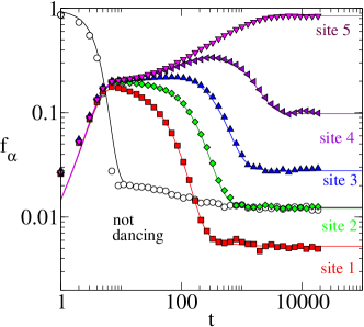
Figure 2: Temporal decision dynamics of the group of bees at $\mu=0,\lambda=0.8$. We show the fraction $f_{\alpha}(t)$ of bees dancing for each of the sites, $\alpha=1,2,\dots,5$, along with the fraction of bees who are not dancing. Solid lines are from the deterministic dynamics, Eqs. (7), markers from simulations started from an all-passive state ($N=400$ bees, averaged over $250$ runs).

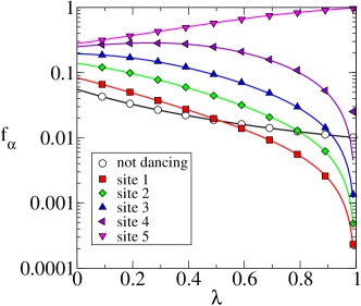
Figure 3: Fraction $f_{\alpha}^{*}$ of bees dancing for each of the sites, $\alpha=1,2\dots,5$, in the long-run, along with the fraction of bees who are not dancing, versus $\lambda$ at fixed $\mu=0$. Solid lines are from the deterministic dynamics, markers from simulations ($N=400$, run for $20000$ steps, averaged over $50$ runs).

III.1 Master equation and dynamics in the deterministic limit

In order to analyze the stochastic process defined by the dynamics of the model, we will write $n_{\alpha}(t)$ for the number of bees dancing for each of the sites at time $t$. We here explicitly include the state $\alpha=0$, i.e. bees not dancing at time $t$. One then has $\sum_{\alpha=0}^{k}n_{\alpha}(t)=N$ for all times $t$. For later convenience we introduce the vector $\mathbf{n}(t)=(n_{0}(t),n_{1}(t),\dots,n_{k}(t))$. The state of the system at time $t$ is therefore fully determined by $\mathbf{n}(t)$. The reduced model defines a Markov process for $\mathbf{n}(t)$, described by the following master equation (see textbooks such as van Kampen (1992) or Gardiner (2009) for details on the master equation formalism)

$$\frac{d}{dt}P_{\mathbf{n}} = \sum_{\alpha=1}^{k}P_{\mathbf{n}-\mathbf{e}_{\alpha}+\mathbf{e}_{0}}T^{+}_{\alpha}(\mathbf{n}-\mathbf{e}_{\alpha}+\mathbf{e}_{0})-P_{\mathbf{n}}\sum_{\alpha=1}^{k}T^{+}_{\alpha}(\mathbf{n})$$

$$+\sum_{\alpha=1}^{k}P_{\mathbf{n}+\mathbf{e}_{\alpha}-\mathbf{e}_{0}}T^{-}_{\alpha}(\mathbf{n}+\mathbf{e}_{\alpha}-\mathbf{e}_{0})-P_{\mathbf{n}}\sum_{\alpha=1}^{k}T^{-}_{\alpha}(\mathbf{n})$$

for the probability $P_{\mathbf{n}}(t)$ of finding the system in state $\mathbf{n}$ at time $t$. $T^{+}_{\alpha}(\mathbf{n})$ here stands for the probability that a randomly chosen bee is inactive and starts dancing for site $\alpha\in\{1,\dots,k\}$ at time $t$, given that the system is in state $\mathbf{n}$. Similarly, $T^{-}_{\alpha}(\mathbf{n})$ is the probability for a randomly chosen individual to be dancing for site $\alpha$ and for it to cease dancing in the subsequent time step. We write $\mathbf{e}_{\alpha}$, $\alpha=0,1,\dots,k$ for the $k+1$ unit vectors, i.e. one has $(\mathbf{e}_{\alpha})_{\beta}=\delta_{\alpha\beta}$ for $\alpha,\beta\in\{0,1,\dots,k\}$. The transition rates are given by

$$T_{\alpha}^{+}(\mathbf{n})=\frac{n_{0}}{N}\left[(1-\lambda)\pi_{\alpha}+\lambda\frac{n_{\alpha}}{N}\right]$$ (3)

and

$$T_{\alpha}^{-}(\mathbf{n})=\frac{n_{\alpha}}{N}\underbrace{q_{0}\left[\frac{\mu}{K}+\frac{1-\mu}{q_{\alpha}}\right]}_{=r_{\alpha}}$$ (4)

respectively, where $\alpha=1,\dots,k$. Technically speaking, this master equation is more appropriate for so-called random sequential updating, in which the states of the $N$ bees are updated one-by-one (and each update would then take a time-step of $1/N$, so that each bee is updated on average once per unit time), see van Kampen (1992); Risken (1996); Gardiner (2009) for details. The pre-factors $n_{\alpha}/N$ in the rates $T_{\alpha}^{\pm}$ here in fact represent the probabilities that a randomly chosen bee is in state $\alpha$. We have verified in numerical simulations that there are no significant differences between the stationary states of the model with parallel and sequential updating respectively, and as we will see below theoretical predictions from our master equation approach agree well with simulations using parallel update rules.

Introducing continuous variables $f_{\alpha}=n_{\alpha}/N$ for $\alpha=0,1,\dots,k$ it is then straightforward to derive a set of deterministic ordinary differential equations in the limit of an infinite system size, $N\to\infty$. This may for example be done by considering

$$\left\langle{\mathbf{n}(t)}\right\rangle=\sum_{\mathbf{n}}\mathbf{n}P_{\mathbf{n}}(t)$$ (5)

and noting that

$$\frac{d\left\langle{\mathbf{n}(t)}\right\rangle}{dt} = \sum_{\alpha=1}^{k}\left[(\mathbf{e}_{\alpha}-\mathbf{e}_{0})T^{+}_{\alpha}(\left\langle{\mathbf{n}}\right\rangle)\right]$$ (6)

$$+\sum_{\alpha=1}^{k}\left[(\mathbf{e}_{0}-\mathbf{e}_{\alpha})T^{-}_{\alpha}(\left\langle{\mathbf{n}}\right\rangle)\right],$$

where we have used a deterministic approximation to write $\left\langle{T^{\pm}_{\alpha}(\mathbf{n})}\right\rangle=T^{\pm}_{\alpha}(\left\langle{\mathbf{n}}\right\rangle)$. This gives

$$\dot{f}_{\alpha}(t)=(1-\rho(t))\left[(1-\lambda)\pi_{\alpha}+\lambda f_{\alpha}(t)\right]-r_{\alpha}f_{\alpha}(t),$$ (7)

for $\alpha=1,\dots,k$, and where $\rho(t)=\sum_{\alpha=1}^{k}f_{\alpha}(t)$. The fraction of bees not dancing at time $t$ is given by $f_{0}(t)=1-\rho(t)$.

III.2 Comparison with simulations

Equations (7) are easily integrated numerically for any fixed choice of the model parameters, and we show a specific example in Fig. 2. We here choose the model parameters as in List et al. (2009), specifically we use $k=5$, $(q_{0},q_{1},...,q_{5})=(0.1,3,5,7,9,10)$, $K=q_{5}$, and $\pi_{1}=...=\pi_{5}=0.05$, as well as $\pi_{0}=0.75$. Our definitions of the transition rates require $q_{0}>0$ and so we choose a small, but non-zero value for $q_{0}$. As mentioned above $q_{0}$ sets the overall time-scale of the model, and is essentially arbitrary, so that the times indicated in Fig. 2 do not necessarily have a direct biological interpretation in terms of e.g. hours, days or the total number of nest inspection flights done by the population. As seen in the figure the theoretical description of Eqs. (7) agrees near perfectly with results from simulations, and reproduces even non-monotonic trajectories faithfully. The stationary state of the system may therefore be determined as a fixed point of Eqs. (7), i.e. as the solution of the $k$ coupled quadratic equations,

$$r_{\alpha}f_{\alpha}^{*}=\left(1-\sum_{\beta=1}^{k}f_{\beta}^{*}\right)\left[(1-\lambda)\pi_{\alpha}+\lambda f_{\alpha}^{*}\right]$$ (8)

for $\alpha=1,\dots,k$, and where we have introduced the notation $f_{\alpha}^{*}$ to denote the fixed-points of (7). These fixed-point equations may in principle be solved numerically, or alternatively, one integrates Eqs. (7) to asymptotic times. We have here followed the latter approach. It is interesting to note that Eqs. (8) can be re-arranged to give

$$f_{\alpha}^{*}=\left[\frac{r_{\alpha}}{1-\rho^{*}}-\lambda\right]^{-1}\bigg{(}1-\lambda\bigg{)}\pi_{\alpha},~{}~{}~{}\alpha=1,\dots,k.$$ (9)

Given that all sites have the same a-priori probability of being found, i.e. that $\pi_{\alpha}$ does not depend on $\alpha\in\{1,\dots,k\}$, and that secondly the rates of dances being terminated decrease with an increasing quality of the sites, $r_{\alpha}<r_{\beta}$ for $\alpha>\beta$, Eqs. (9) reveal immediately, that a site is the more populated on the deterministic level, the higher its quality, i.e. $f_{1}^{*}<f_{2}^{*}<\dots<f_{k}^{*}$, in-line with the results of LES. We also note that for $\lambda=1$ the only possible fixed point is one at which $f_{\alpha}^{*}=0$ for all $\alpha=1,\dots,k$.

To test our theoretical predictions regarding the stationary state we show the asymptotic values of $f_{0}^{*},f_{1}^{*},...,f_{5}^{*}$ as a function of the model parameter $\lambda$ in Fig. 3, and again simulations confirm that our mean-field description accurately reproduces the behavior of the agent-based model in a wide range of model parameters. Figure 3 also reveals that the behavior of the simplified model is very similar to that of the original model by LES (see Hypothesis 1 and Figs. 1-3 of List et al. (2009)): if the bees assess the quality of the sites independently before dancing for a given site, i.e. if $\mu=0$, then the best site is retrieved successfully over a wide range of values for the parameter $\lambda$. In-line with the findings of List et al. (2009), an increased amount of interdependence between the bees (high values of $\lambda$) increases the chances of finding the best nest site, as indicated by the proportion of bees, $f_{5}^{*}$, dancing for the best site $\alpha=5$.

Having established the correctness of our theoretical approach, we can now push the analysis further, and assess the decision-dynamics of the bees throughout the parameter space defined by $\lambda$ and $\mu$. To this end we have integrated Eqs. (7) to large times ($t=10^{5}$) for approximately $1.6\cdot 10^{5}$ different combinations of $\lambda$ and $\mu$, equally spaced in the unit square, and have computed the difference $\Delta=f_{5}^{*}-f_{4}^{*}$ between the fraction of bees dancing for the best site and the fraction of bees dancing for the second-best site. $\Delta$ therefore ranges in the interval $[0,1]$, and high values of $\Delta$ indicate that the best site ($\alpha=5$) is identified with a high accuracy by the population of bees. Results are shown in Fig. 4, and confirm that a reliable convergence to the best site can only be achieved in the presence of both, a sufficient degree of independence in the assessment of nest-sites and interdependence between the different individuals. This is a confirmation of the second main hypothesis of List et al. (2009). The best retrieval of the optimal site is found at low values of $\mu$ (high independence) and large $\lambda$ (high interdependence). In order to check for convergence we have also analyzed data from an integration of Eqs. (7) only up to $t=10^{4}$. The location of the different lines in Fig. 4 remains unchanged at this lower time, so that we conclude that the stationary state has already been reached much earlier than at $t=10^{5}$.

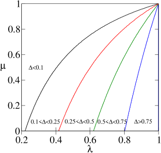
Figure 4: Quality of the retrieval of the best site, as measured by $\Delta$ (see main text), throughout the parameter space. High values of $\Delta$ indicate a high accuracy in identifying the best nest site. Results are from an integration of Eqs. (7), using a first-order Euler-forward scheme with a time-stepping of $dt=0.1$, integrated up to time $t=10^{5}$.

III.3 Size-limitations of best-site retrieval

The deterministic dynamics defined by Eqs. (7) approaches a stationary state in which the proportion of bees populating the best site is higher than that of any other site. The description in terms of these deterministic equations is however only valid in the formal limit of an infinite population of bees, i.e. if $N\to\infty$. In small populations stochastic effects may instead dominate the decision making, and as observed by LES convergence to a sub-optimal state may occur. To characterize these finite-size effects one may look at a system at a fixed size $N$ and at fixed model parameters $\lambda$ and $\mu$. At any given time, the state of the system is described by the (re-scaled) population vector $(n_{1}(t)/N,n_{2}(t)/N,\dots,n_{k}(t)/N)$, and the dominating choice at any given time may well be different from the optimal site, i.e. it may well be that the most-populate site at time $t$ is not actually the best site $\alpha=k$. This is the case whenever there is an index $\alpha\in\{1,\dots,k-1\}$ such that $n_{\alpha}(t)>n_{k}(t)$. It is therefore instructive to look at the joint and marginal distributions of the values $(n_{1}(t)/N,n_{2}(t)/N,\dots,n_{k}(t)/N)$ sampled over time and from different simulation runs. We first address the marginals, and the resulting histograms are shown for a particular choice for $\lambda$ and $\mu$ and for a relatively large system ($N=2500$) in Fig. 5. For optical convenience we suppress the results for the second and fourth sites respectively. As seen in the figure there may be a considerable overlap between the distributions corresponding to the optimal site and the sub-optimal ones, so that the population of bees may well misidentify the best site with a significant probability. Since the variance of the distributions shown in Fig. 5 scales as $N^{-1}$ by virtue of the central limit theorem, this effect will generally be the less pronounced the larger the swarm size. For large swarms the individual population levels fluctuate less, resulting in sharper peaks, and a lesser chance of favoring a sub-optimal state. This is a special case of what is known as ‘Condorcet’s jury theorem’ (see List et al. (2009) and references therein), and the effect is illustrated in Fig. 6, where we plot the frequencies with which the different sites are favored in simulations at fixed model parameters and system sizes. More precisely, in each simulation run, we check for each time step which site is the most populated at this moment in time, and from this construct the histograms shown in the figure, indicating how frequently the different sites come up as the most-populated one (the ‘site’ $\alpha=0$ (passive bees) is here not taken into account). We take a simple majority as sufficient criterion for a consensus, although this is admittedly a rather weak definition (termed ‘weak consensus criterion’ by LES), stronger conditions are discussed in List et al. (2009). As seen in the figure site $\alpha=5$ comes up with the highest rate for the model parameters chosen in the figure, but there is also a considerable probability for the sub-optimal sites to have the most bees dancing for them. From our simulations we conclude that this effect is relevant mostly at small independence ($\mu$ close to unity), and tends to become stronger the smaller the interdependence parameter $\lambda$, and/or the smaller the swarm.

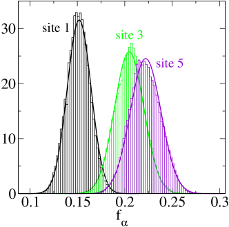
Figure 5: The population levels $n_{\alpha}/N$ are stochastic quantities for finite systems, we here show their distributions for sites $\alpha=1$, $\alpha=3$ and $\alpha=5$ for fixed model parameters $\mu=0.95,\lambda=0.4$. The system-size is $N=2500$. Measurements in simulations are taken after an equilibration period of $10000$ time-steps, and results are averaged over $20$ independent runs. Solid lines are the theoretical predictions derived from Eqs. (15), i.e. they are Gaussian distributions of mean $f_{\alpha}^{*}$ and with variances $\overline{\Lambda}_{\alpha\alpha}$.

These finite-size stochastic effects can actually be understood analytically, based on an approach using the so-called van Kampen expansion in the inverse system size. In the remainder of this section we will describe some of the intermediate steps, but will not go through the derivation in all detail, as the necessary mathematics is readily available in the literature van Kampen (1992). As a starting point we separate off stochastic fluctuations from the deterministic solution $\mathbf{f}(t)$ of Eqs. (7):

$$\frac{\mathbf{n}(t)}{N}=\mathbf{f}(t)+\frac{1}{\sqrt{N}}\bm{\xi}(t),$$ (10)

anticipating that the magnitude of deviations from the deterministic system scales as $N^{-1/2}$. One then proceeds as described in van Kampen (1992), and expands the master equation (LABEL:eq:master) in powers of $N^{-1/2}$. In lowest order one recovers the deterministic dynamics of Eqs. (7), and in next-to-leading order one has

$$\dot{\bm{\xi}}=\mathbb{J}\bm{\xi}+{\mbox{\boldmath$\eta$}}$$ (11)

in the stationary regime, where a fixed-point of the mean-field trajectory has been assumed. The matrix $\mathbb{J}$ is the $k\times k$ Jacobian of the deterministic dynamics at this fixed point, i.e. one has

$$J_{\alpha\beta}=-\left[(1-\lambda)\pi_{\alpha}+\lambda f_{\alpha}^{*}\right]+\left[\lambda(1-\rho^{*})-r_{\alpha}\right]\delta_{\alpha\beta}$$ (12)

for $\alpha,\beta\in\{1,\dots,k\}$. The quantity $\eta$ in (11) is Gaussian white noise of zero mean and with the following diagonal covariance matrix between components

$$\left\langle{\eta_{\alpha}(t)\eta_{\beta}(t^{\prime})}\right\rangle=\delta_{\alpha\beta}\Gamma_{\alpha\beta}\delta(t-t^{\prime}),$$ (13)

where

$$\Gamma_{\alpha\alpha}=(1-\rho^{*})\left[(1-\lambda)\pi_{\alpha}+\lambda f_{\alpha}^{*}\right]+r_{\alpha}f_{\alpha}^{*}.$$ (14)

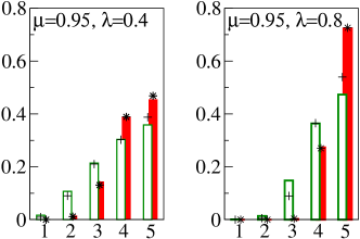
Figure 6: Probabilities for the different sites $\alpha$ to be the most-populated one. Filled bars show results from simulations for $N=2500$, averaged over $20$ samples, open green bars are for $N=400$ (averaged over $50$ samples); the measurement period starts after $10000$ time-steps in the simulations. The stars and crosses show the estimates from the analytical theory in the first order of the system-size expansion, as described in the text.

These results can also be read off from the general expressions given for example in Boland et al. (2008). Equation (11) describes an multi-component Ornstein-Uhlenbeck process Gardiner (2009), and the co-variance matrix of the random variables $\xi_{\alpha}(t)$ hence has a relatively simple time-evolution. In particular if we define $\Lambda_{\alpha\beta}(t)=\left\langle{\xi_{\alpha}(t)\xi_{\beta}(t)}\right\rangle$, then one has Risken (1996)

$$\dot{\Lambda}_{\alpha\beta}=\sum_{\gamma=1}^{k}\left[J_{\alpha\gamma}\Lambda_{\gamma\beta}+J_{\beta\gamma}\Lambda_{\gamma\alpha}\right]+\Gamma_{\alpha\beta},$$ (15)

for $\alpha,\beta\in\{1,\dots,k\}$. Denoting the fixed-point of these equations by $\overline{\Lambda}$ one has asymptotically

$$P\left(\frac{\mathbf{n}}{N}=\mathbf{x}^{*}+N^{-1/2}\bm{\xi}\right)$$ (16)

$$= {\cal N}\exp\left(-\frac{1}{2}\sum_{\alpha\beta}\xi_{\alpha}(\overline{\Lambda}^{-1})_{\alpha\beta}\xi_{\beta}\right)$$

for the distribution of the population vector $\mathbf{n}$. ${\cal N}$ is a normalization factor. Within our approximation (consisting in the truncation of the van-Kampen expansion after the sub-leading order) this distribution is Gaussian, with a co-variance matrix $\overline{\Lambda}$. It is here appropriate to point out that, within this approximation, the expression in Eq. (16) characterizes the statistics of the system at finite sizes fully, as both the variances of the individual components of $\mathbf{n}$ and their correlations are taken into account. This allows one to estimate mathematically how often each of the sites will be the ‘winner’ of the quorum decision, for example, using the weak consensus criterion of LES.

In order to generate these semi-analytical estimates characterizing the finite-size effects of the system, we have first integrated the master equation to asymptotic times to extract the fixed-point vector $\mathbf{f}^{*}$. From this one computes the Jacobian $\mathbb{J}$, and the above matrix $\Gamma$. Integrating Eqs. (15) then gives $\overline{\Lambda}$. A comparison of these findings against simulations is shown in Fig. 5, and as seen in the figure reasonably good agreement is achieved so that we conclude that our theoretical approach gives accurate estimates for the variances of the $\{n_{\alpha}\}$, at least for the model parameters used in Fig. 5. The matrix $\overline{\Lambda}$ is then inverted, and subsequently results are inserted into Eq. (16), and numerical integration of the resulting multi-variate Gaussian distribution then produces analytical estimates for the probabilities for the different sites $\alpha\in\{1,\dots,k\}$ to be the most-populated one. These semi-analytical results are compared with simulations in Fig. 6, and the agreement is found to be reasonable, especially at large system sizes. We would here like to stress that we have not been able to obtain agreement of the level shown in Figs. 5 and 6 for all values of the model parameters. In particular if $\lambda$ is large, deviations can be significant, even for the largest system-sizes we have tried (up to $10^{4}$). We attribute this to remaining finite-size corrections (truncating the van Kampen expansion might not be justified in these circumstances), to equilibration effects, or to numerical inaccuracies in integrating the $5$-dimensional Gaussian distribution (16). Also note that the Gaussian approximation becomes inaccurate if any of the $f_{\alpha}^{*}$ are near the upper or lower limits of the interval $[0,1]$. In simulations no $n_{\alpha}/N$ can ever come out negative or exceed unity, these boundary effects are not captured by the first-order approximation of the van Kampen expansion. As a final note in this section, we point out that the stronger consensus criterion discussed in List et al. (2009) can be studied based on Eq. (16) as well, as this equation provides a Gaussian estimate for the joint distribution of all $k$ population levels. We have however not tried to do so here.

IV Spatial model

IV.1 Model definitions and simulation results

In this section we consider a spatial extension of the simplified model. To this end we place the dancing or resting bees on a square lattice of lateral extension $L$, and apply periodic boundary conditions for simplicity. The total system is composed of $N=L\times L$ agents. The update dynamics is as in the simplified model described above, the only difference is that any given non-dancing bee is only affected by bees in its direct neighborhood when it decides to start dancing for a given site, and not by the entire population. Specifically, the above fractions $f_{\alpha}(t)$, of bees dancing for site $\alpha$, now carry a dependence on space, i.e. we introduce $f_{\alpha}(\mathbf{x},t)$ as the fraction of bees on nearest neighbor lattice sites of $\mathbf{x}$ dancing for site $\alpha$. More precisely we have $f_{\alpha}(\mathbf{x},t)=\frac{1}{4}\sum_{\mathbf{y}\sim\mathbf{x}}\delta_{\alpha,s_{\mathbf{y}}(t)}$, where the sum over $\mathbf{y}$ extends over the four nearest neighbors of $\mathbf{x}$. A bee located at lattice site $\mathbf{x}$ then takes into account the $f_{\alpha}(\mathbf{x},t),~{}\alpha=1,\dots,k$ when it considers to commence a dance. The rate with which it starts dancing for site $\alpha$ is then given by $p_{\alpha}(\mathbf{x},t)=(1-\lambda)\pi_{\alpha}+\lambda f_{\alpha}(\mathbf{x},t)$. Apart from this modification the dynamics proceeds exactly as in the non-spatial model.

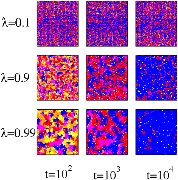
Figure 7: Pattern formation and coarsening dynamics in the spatial model at $\mu=0$. The panels show the configuration of the system at $\lambda=0.1,0.9$ and $\lambda=0.99$ respectively, and at different times of the simulation runs (i.e. after $t=10^{2},10^{3},10^{4}$ sweeps). Simulations are performed on a square lattice with $L\times L=100^{2}$ agents, with periodic boundary conditions, and started from an all-passive initial condition. The different colors indicate different states of the individual bees, with white squares corresponding to bees who are not dancing, and filled squares to bees dancing for a particular site as indicated by the different colors. Lighter colors correspond to the states with low quality, and the black (blue on-line) areas to bees dancing for the best site. The optical impression may sometimes not reflect the actual proportions of bees dancing for the actual sites, accurately, e.g. in the top row we have $27\%$, $31\%$ and $31\%$ of bees dancing for site $5$, in the bottom row these numbers are $24\%$, $52\%$ and $97\%$ at the three different times respectively.

One should point out that we are here departing from a realistic modelling of the decision making of bees, as space in our model is isotropic and invariant against translations. No special point in space is designated as the entrance into the hive (where incoming bees would arrive when they return from site-inspection flights). However, as discussed in the conclusions, the dynamics proposed by LES can be understood as a more general model for decision making, applicable also in contexts different from the nest-site choice of bees, so that it is worthwhile investigating the spatial extension discussed in the present section.

Results from simulations are shown in Fig. 7. When the simulations are initiated, all bees are passive, i.e. not dancing. As seen in the figure non-trivial large-scale patterns emerge for sufficiently large interdependence, see especially the configurations corresponding to $\lambda=0.9$ and $\lambda=0.99$ at intermediate times $t\approx 100$. Inspecting the system at later times (right-most snapshots in Fig. 7) shows that these patterns are of a transient nature only, and a coarsening dynamics to a broad consensus on the best nest-site emerges in the spatial system. Interestingly, transient structures do depend on the interdependence parameter $\lambda$: strong interdependence promotes large domains of agreement on one of the different nest sites, whereas at small $\lambda$ no such large-scale areas of consensus are found. We should here also point out that these patterns do seem to depend on the initial conditions chosen, e.g. if we initiate the system from a state where all bees are active and dancing for randomly chosen sites, then the formation of domains seems to be far less pronounced.

IV.2 Analytical approaches

In order to make further progress towards an analytical description of the spatial system, we here extend the above master equation approach, and study the following spatial analogue of the mean-field dynamics (7) of the non-spatial system,

$$\dot{\varphi}_{\alpha}(\mathbf{x},t) = \bigg{(}1-\rho(\mathbf{x},t)\bigg{)}\bigg{[}(1-\lambda)\pi_{\alpha}$$ (17)

$$+\lambda(\Delta\varphi_{\alpha}(\mathbf{x},t)+\varphi_{\alpha}(\mathbf{x},t))\bigg{]}$$

$$-r_{\alpha}\varphi_{\alpha}(\mathbf{x},t)$$

for $\alpha=1,\dots,k$. Here $\varphi_{\alpha}(\mathbf{x},t)$ is a continuous-valued field defined on the lattice points of the system, and indicates the probability of finding the agent at site $\mathbf{x}$ in state $\alpha$. The $\varphi_{\alpha}(\mathbf{x},t)$ are hence coarse-grained order parameters, but no continuum limit in space is implied. Note that Eqs. (17) are coupled through $\rho(\mathbf{x},t)=\sum_{\alpha=1}^{k}\varphi_{\alpha}(\mathbf{x},t)$. The quantity $\Delta\varphi_{\alpha}(\mathbf{x},t)$ is the lattice Laplacian, i.e. we have $\Delta\varphi_{\alpha}(\mathbf{x},t)=\left(\frac{1}{4}\sum_{\mathbf{y}\sim\mathbf{x}}\varphi_{\alpha}(\mathbf{y},t)\right)-\varphi_{\alpha}(\mathbf{x},t)$. The term $\Delta\varphi_{\alpha}(\mathbf{x},t)+\varphi_{\alpha}(\mathbf{x},t)$ in the above expression of the right-hand-side of Eqs. (17) is thus equal to $\frac{1}{4}\sum_{\mathbf{y}\sim\mathbf{x}}\varphi_{\alpha}(\mathbf{y},t)$, and describes the total density of individuals in state $\alpha$ in the neighbourhood of $\mathbf{x}$.

Results from a numerical integration of these equations are shown in Fig. 8, for a case in which random initial conditions are chosen to introduce spatial inhomogeneity. We find that the prediction from the spatial and non-spatial deterministic dynamics do not differ much, and that Eqs. (17) capture the qualitative behavior of the dynamics, but that no quantitative agreement is achieved. The dynamics on the lattice appears to converge more slowly than in the well-mixed system, and than predicted by Eqs. (17). These deviations point to the observation that while neglecting fluctuations was justified in the well-mixed non-spatial system, stochasticity is relevant in the two-dimensional system. In order to examine the spatial structures one obtains from Eqs. (17) we show a number of snapshots in Fig. 9. It should be noted that these were taken from random initial conditions, with $5\%$ of the bees active, as explained in the figure caption. Homogeneous initial conditions in the noise-less equations (17) do not lead to any pattern formation, as the field trivially remains homogeneous for all times. Fig. 9 shows domain formation similar to that in Fig. 7, but the extent to which the patterns of the agent-based model are reproduced by the deterministic dynamics of Eqs. (17) is at present still undetermined, and will be left for future work. Integrating Eqs. (17) at $\lambda=0.9$ for example (not shown) yields results very similar to those at $\lambda=0.99$, whereas in the agent-based model systematic differences are found between those two cases, as seen in Fig. 7. To understand the relation between the agent-based model, and the effective dynamics in terms of continuous fields a detailed analysis of e.g. correlation lengths and other statistical features of the spatio-temporal patterns will be required. Based on the observations reported in Fig. 8 it may well be the case that a more accurate description will make it necessary to take into account fluctuations around the deterministic dynamics. We have not attempted to pursue this further, but based on existing work in voter models and related spatial agent-based systems (see e.g. Dornic et al. (2005), Reichenbach et al. (2008) or Dall’Asta & Galla (2008) and references therein), one may consider the following stochastic extension

$$\dot{\varphi}_{\alpha}(\mathbf{x},t) = \bigg{(}1-\rho(\mathbf{x},t)\bigg{)}\bigg{[}(1-\lambda)\pi_{\alpha}$$ (18)

$$+\lambda(\Delta\varphi_{\alpha}(\mathbf{x},t)+\varphi_{\alpha}(\mathbf{x},t))\bigg{]}$$

$$-r_{\alpha}\varphi_{\alpha}(\mathbf{x},t)+\zeta_{\alpha}(\mathbf{x},t),$$

where $\zeta_{\alpha}(\mathbf{x},t)$ is Gaussian noise of zero mean and with correlations

$$\left\langle{\zeta_{\alpha}(\mathbf{x},t)\zeta_{\beta}(\mathbf{x}^{\prime},t^{\prime})}\right\rangle=\delta_{\alpha\beta}B_{\alpha\alpha}\delta(\mathbf{x}-\mathbf{x}^{\prime})\delta(t-t^{\prime}),$$ (19)

where

$$B_{\alpha\alpha} = \bigg{(}1-\rho(\mathbf{x},t)\bigg{)}\bigg{[}(1-\lambda)\pi_{\alpha}$$ (20)

$$+\lambda(\Delta\varphi_{\alpha}(\mathbf{x},t)+\varphi_{\alpha}(\mathbf{x},t))\bigg{]}$$

$$+r_{\alpha}\varphi_{\alpha}(\mathbf{x},t).$$

This covariance matrix is an analogue of (14) and can be obtained following Dall’Asta & Galla (2008). Due to the multiplicative noise, it is difficult to integrate equations (18,19,20) numerically, so that we do not present any further results here, but only mention that one approach might be to extend recently developed methods Moro (2004); Dornic et al. (2005) to the case of multiple fields. We would like to stress that (17,18,19,20) are not to be understood as a rigorously valid description of the spatial system. We feel that further more detailed considerations of the continuous description of the model are beyond the scope of the present paper, but would like to mention that several approaches could be considered in future work: explicit diffusion (particle exchange between neighbouring sites) could be taken into account, and a continuum limit could be derived along the lines of Reichenbach et al. (2008), using a Kramers-Moyal expansion (see Gardiner (2009), and also Traulsen et al. (2006)). Alternatively systematic expansions for spatial models with a large number of individuals per lattice site can be found in Lugo & McKane (2008), where a van Kampen system-size expansion is used van Kampen (1992).

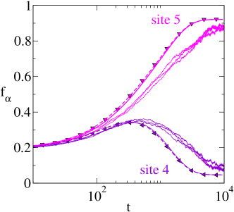
Figure 8: Fraction of bees dancing for the best and second-best sites respectively (upper curves resp. lower curves). The smooth solid lines show results from an integration of the deterministic dynamics of Eqs. (17), the dashed lines are from an integration of the non-spatial deterministic dynamics given by Eqs. (7). Noisy lines show three independent simulation runs of the spatial agent-based model for $N=100^{2}$ agents. Markers are from simulations of the non-spatial model ($N=10^{4}$, average over $10$ samples). Model parameters are $\mu=0,\lambda=0.9$, in the initial state all bees are active and dance for randomly chosen sites.

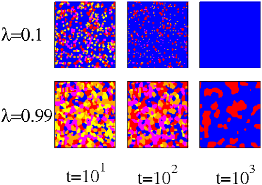
Figure 9: Field configurations generated from a numerical integration of Eqs. (17) at $\mu=0$, started from an initial condition in which 95$\%$ of all bees are passive, and the remaining randomly chosen $5\%$ of bees dance for randomly chosen sites (i.e. at each lattice point draw one $\alpha\in\{1,\dots,k\}$ and set $\varphi_{\alpha}(\mathbf{x},t=0)=1$, and $\varphi_{\beta}(\mathbf{x},t)=0$, for all $\beta\neq\alpha$). Integration is performed using a first-order Euler-forward scheme with a time stepping of $dt=0.1$. The different colors indicate the dominant state, i.e. at each lattice site $\mathbf{x}$ and each moment in time we identify $\alpha$ such that $\varphi_{\alpha}=\mbox{max}\{\varphi_{1}(\mathbf{x},t),...,\varphi_{k}(\mathbf{x},t)\}$. Color coding is as in Fig. 7. The size of the lattice is $100\times 100$.

V Conclusions

The model of the nest-site choice dynamics in swarms of honeybees by LES is a beautiful example of a biologically inspired agent-based model, which can be solved with techniques originally developed in statistical physics. As we have shown, only modest modifications to the dynamics proposed by LES are required to make the model analytically tractable. The reduced model is Markovian in a relatively simple configuration space, and we have used a master equation approach to derive a deterministic continuous-time description in terms of a set of coupled differential equations. These can be integrated numerically, and alternatively their fixed points can be obtained as a the solution of a small set of quadratic equations. The reduction may limit the degree of realism in the model, but as we have shown the simpler model reproduces most, if not all features of the original dynamics. In particular it confirms that in order for the population of bees to accurately identify the best site for a future nest, both independence in the assessment of the quality of the nest sites and interdependence between the bees is necessary. Based on our analytical solutions we are able to characterize the stationary state of the system in the entire parameter space spanned by the variables $\lambda$ and $\mu$ representing the degree of interdependence and the degree of independence respectively, without the need to perform extensive agent-based simulations. While the analytical description is mostly on the deterministic level, a systematic approach to finite-size effects is feasible based on an expansion in the inverse system size. This allows one, within the limitations discussed above, to obtain estimates for the frequency with which finite swarms of bees will reach a consensus for each of the potential nest-sites, including the sub-optimal ones.

We have also extended the model to a spatial arrangement on a simple square lattice, and have demonstrated in computer simulations that the interacting agent model gives rise to non-trivial transient patterns before a coarsening dynamics towards a consensus on the best nest-site sets in. These patterns are observed only at moderate to high interdependence of the bees. Finally, we have discussed a simple set of reaction-diffusion like equation derived from the master equation of the spatial system. These equations capture some of the characteristics of the spatial patterns formed in the agent-based model, but further work is required to determine whether they faithfully capture statistical features of these patterns. It is important to note that we have not taken into account explicit diffusion though, as no hopping of agents or particle exchange is considered in our model. A more detailed analysis of the effects of multiplicative noise on the field equations is a further interesting point, which needs a more detailed investigation.

We would finally like to comment on possibilities to account for uncertainties in the quality assessment as LES do in their original model (parametrized by $\sigma$). One way of doing this may be to formally increase the number of sites in our simplified model, i.e. to introduce several ‘copies’ of each site. E.g. for a given site $\alpha$, one could introduce formal copies $\alpha^{(1)},\alpha^{(2)},...$ and then draw formal quality factors $q_{\alpha^{(1)}},q_{\alpha^{(2)}},\dots$ from some distribution centered around the true quality of site $\alpha$, and with a standard deviation given by the uncertainty parameter $\sigma$. This would mathematically increase the number of ‘sites’ in the model, even though all $\alpha^{(j)}$, $j=1,2,\dots$ would refer to the same real-world site, i.e. the total number of bees dancing for site $\alpha$ would be computed as $n_{\alpha}^{tot}=\sum_{j}n_{\alpha^{(j)}}$.

Other points of further research might address the model in spatial arrangements different from a simple two-dimensional regular lattice. One may here for example study the effects of the topology of the network of interactions on the convergence and consensus properties. In this context the model proposed by LES and the simplified dynamics discussed in the present paper could probably be interpreted more generally as a model for the interplay of independence and interdependence in the decision making of groups, where the specific application may not necessarily be limited to the nest-site choice of honeybees. LES give an example towards the end of their paper, relating to the choice of restaurants by humans, and similarly many other situations, where individuals have to make strategic choices, for example in the social sciences and in game theory may potentially be modeled using similar dynamics. The analytical approaches developed in the present paper may here be useful for to characterize the outcome of the decision making processes in such models.