Feynman and Squeezed States

Abstract

In 1971, Feynman et al. published a paper on hadronic mass spectra and transition rates based on the quark model. Their starting point was a Lorentz-invariant differential equation. This equation can be separated into a Klein-Gordon equation for the free-moving hadron and a harmonic oscillator equation for the quarks inside the hadron. However, their solution of the oscillator equation is not consistent with the existing rules of quantum mechanics and special relativity. On the other hand, their partial differential equation has many other solutions depending on boundary conditions. It is noted that there is a Lorentz-covariant set of solutions totally consistent with quantum mechanics and special relativity. This set constitutes a representation of the Poincaré group which dictates the fundamental space-time symmetry of particles in the Lorentz-covariant world. It is then shown that the same set of solutions can be used as the mathematical basis for two-photon coherent states or squeezed states in quantum optics. It is thus possible to transmit the physics of squeezed states into the hadronic world. While the time-like separation is the most puzzling problem in the covariant oscillator regime, this variable can be interpreted like the unobserved photon in the two-mode squeezed state which leads to an entropy increase.

I Introduction

Since Einstein’s formulation of special relativity in 1905, the most important development in physics is the formulation of quantum mechanics resulting in Heisenberg’s uncertainty principle.

For solving practical problems, the Schrödinger wave equation is commonly used. For scattering problems, we use running-wave solutions. For bound states, we obtain standing-wave solutions with their boundary conditions. Indeed, this localization boundary condition leads to discrete energy levels.

For scattering problems, we now have Lorentz-covariant quantum field theory with its scattering matrix formalism and Feynman diagrams. Since quantum field theory was so successful that there had been attempts in the past to understand bound-state problems using the S matrix method. However, it was noted from the calculation of the neutron-proton mass difference from Dashen and Frautchi that the S-matrix method does not guarantee the localization of the bound-state wave functions dyson65 ; kim66 .

While the localization boundary condition is the main problem for the bound state, the question is whether this issue is covariant under Lorentz transformations. We know the hydrogen has its localized wave function, but how would this appear to the observer on a train? One way to reduce this difficulty is to study harmonic oscillators, because the oscillator system has its built-in boundary condition. For this reason, there had been many attempts in the past to make the harmonic oscillator Lorentz-covariant.

In order to understand the hadronic mass spectra and hadronic transition rates in the quark model, Feynman et al. in 1971 published a paper containing the following Lorentz-invariant differential equation fkr71 .

$$\left\{-\frac{1}{2}\left[\left(\frac{\partial}{\partial x^{a}_{\mu}}\right)^{2}+\left(\frac{\partial}{\partial x^{b}_{\mu}}\right)^{2}\right]+\frac{1}{16}\left(x^{a}_{\mu}-x^{b}_{\mu}\right)^{2}+m_{0}^{2}\right\}\phi\left(x^{a}_{\mu},x^{b}_{\mu}\right)=0,$$ (1)

for a hadron consisting of two quarks bound-together harmonic oscillator potential. The space-time quark coordinates are $x^{a}_{\mu}$ and $x^{b}_{\mu}$. They then wrote down the equation

They wrote down the hadronic and quark separation coordinates as

$$X_{\mu}=\frac{1}{2}\left(x^{a}_{\mu}+x^{b}_{\mu}\right),$$

$$x_{\mu}=\frac{1}{2\sqrt{2}}\left(x^{a}_{\mu}-x^{b}_{\mu}\right),$$ (2)

respectively, and $\phi\left(x^{a}_{\mu},x^{b}_{\mu}\right)$ as

$$\phi\left(x^{a}_{\mu},x^{b}_{\mu}\right)=f\left(X_{\mu}\right)\psi\left(x_{\mu}\right).$$ (3)

Then the differential equation can be separated into the following two equations.

$$\left\{\left(\frac{\partial}{\partial X_{\mu}}\right)^{2}+m_{0}^{2}+(\lambda+1)\right\}f\left(X_{\mu}\right)=0,$$ (4)

for the hadronic coordinate, and

$$\frac{1}{2}\left\{-\left(\frac{\partial}{\partial x_{\mu}}\right)^{2}+x_{\mu}^{2}\right\}\psi\left(x_{\mu}\right)=(\lambda+1)\psi\left(x_{\mu}\right),$$ (5)

for the coordinate of quark separation inside the hadron.

The differential equation of Eq.(4) is a Klein-Gordon equation for the hadronic coordinate. The Klein-Gordon equation is Lorentz-invariant and is the starting point for quantum field theory for scattering processes with Feynman diagrams. This aspect of physics is well known. In the present case, the solution takes the form

$$f(X)=\exp{\left(\pm iP\cdot X\right)},$$ (6)

with

$$-P^{2}=m_{0}^{2}+(\lambda+1).$$ (7)

We are using here the space-favored metric where $P^{2}=\left(P_{x}^{2}+P_{y}^{2}+P_{z}^{2}-E^{2}\right)$. The hadronic mass is thus determined from $m_{0}$ and $\lambda$. The $\lambda$ parameter is determined from the oscillator equation of Eq.(5) for the internal space-time coordinate. The internal quark motion determined the hadronic mass, according to Feynman et al.

Indeed, the differential equation of Eq.(1) contains the scattering-state equation for the hadron, and the bound-state equation for the quarks inside the hadron. The differential equation of Eq.(5) is also a Lorentz-invariant equation. The problem is that the set of solutions given by Feynman et al. in their 1971 paper is not consistent with the existing rules of physics. This is the reason why this paper is not well known.

However, this does not exclude other sets of solutions. The solutions can take different forms depending on the separable coordinate systems with their boundary conditions. Indeed, there is a set of oscillator solution that can constitute a representation of the Poincaré group, particularly that of Wigner’s little group which dictates the internal space-time symmetry of the particles in the Lorentz-covariant world wig39 ; kno79 . We choose to call this set of solutions the Poincaré set.

If we ignore the time-like variable in Eq.(5), it is the Schrödinger-type equation for the three-dimensional harmonic oscillator. If we ignore it, the equation loses its Lorentz invariance. The problem is how to deal with the time-separation variable, while it is not even mentioned in the present form of quantum mechanics. If we believe in Einstein, this variable exists wherever there is a spacial separation like the Bohr radius. However, we pretend know about it in the present form of quantum mechanics.

In this report, we give an interpretation to this variable based on the lessons we learn from quantum optics. For this purpose, we show first that the Poincaré set for the covariant harmonic oscillator can be used for mathematical basis for two-photon coherent states or squeezed states yuen76 . In other words, the squeezed states can be constructed from the Lorentz-invariant differential equation of Eq.(5).

We then establish that the longitudinal and time-like excitations in the covariant harmonic oscillator system can be translated into the two-photon coherent state. We know what happens when one of the two photons is not observed. The result is an increase in entropy ekn89 . We can then go back to the covariant oscillator and give a similar interpretation to the time-separation variable which is not observed in the present form of quantum mechanics,

In Sec. II, we introduce the set of solutions of Eq.(5) which constitutes a representation of the Poincarǵroup. We then study the space-time geometry of its Lorentz covariance. In Sec. III, it is shown that the oscillator differential equation of Eq.(5) can serve as the starting equation for squeezed states in quantum optics, and also that this Poincaré set serves as the mathematical basis for the two-photon coherent state. In Sec. IV, we give a physical interpretation to the time-separation variable in terms of Feynman’s rest of the universe, which has a concrete physical interpretation in quantum optics.

II Lorentz Boosts as Squeeze Transformations

In 1979, Kim, Noz, and Oh published a paper on representations of the Poincaré group using a set of solutions of the oscillator equation of Eq.(5) kno79 . Later in 1986, Kim and Noz in their book knp86 noted that this set corresponds to a representation of Wigner’s $O(3)$-like little group for massive particles. If a particle has a non-zero mass, there is a Lorentz frame in which the particle is at rest. Wigner’s little group then becomes that of the three-dimensional rotation group, which is very familiar to us.

The Lorentz-covariant solution of the Lorentz-invariant differential equation contains both space-like and time-like wave components, but we can keep the time-like component to its ground state. The wave function thus retains the $O(3)$-like symmetry. The solution takes the form

$$\psi(x,y,z,t)=\left\{\left(\frac{1}{\pi}\right)^{1/4}\exp{\left(\frac{-t^{2}}{2}\right)}\right\}\psi(x,y,x).$$ (8)

As for the spatial part of the differential equation, it is the equation for the three-dimensional oscillator. We can solve this equation with both the Cartesian and spherical coordinate systems. If we use the spherical system with $(r,\theta,\phi)$ as the variables, the solution should take the form

$$\psi(x,y,z)=R_{\lambda,\ell}(r)Y_{\ell,m}(\theta,\phi)\exp{\left\{-\left(\frac{x^{2}+y^{2}+z^{2}}{2}\right)\right\}},$$ (9)

where $Y_{\ell,m}(\theta,\phi)$ is the spherical harmonics, and $R_{\lambda,\ell}(r)$ is the normalized radial wave function with $r=\sqrt{x^{2}+y^{2}+z^{2}}.$ The $\lambda$ and $\ell$ parameters specify the mass and the internal spin of the hadron respectively, as required by Wigner’s representation theory wig39 ; knp86 .

If we use the Cartesian coordinate systems, and the solution can be written as

$$\psi(x,y,z)=\left[\frac{1}{\pi\sqrt{\pi}2^{(a+b+n)}a!b!n!}\right]^{1/2}H_{a}(x)H_{b}(y)H_{n}(z)\exp{\left\{-\left(\frac{x^{2}+y^{2}+z^{2}}{2}\right)\right\}},$$ (10)

where $H_{n}(z)$ is the Hermite polynomial of $z$. Since the three-dimensional oscillator system is separable in both the spherical and Cartesian coordinate systems, the wave function of Eq.(9) can be written as a linear combination of the solutions given in Eq.(10), with $\lambda=a+b+n.$

When we boost this solution along the $z$ direction, the Cartesian form of Eq.(10) is more convenient. Since the transverse $x$ and $y$ coordinates are not affected by this transformation, we can separate out these variables in the oscillator differential equation of Eq.(5), and consider the differential equation

$$\frac{1}{2}\left\{\left[-\left(\frac{\partial}{\partial z}\right)^{2}+z^{2}\right]-\left[-\left(\frac{\partial}{\partial t}\right)^{2}+t^{2}\right]\right\}\psi(z,t)=n\psi(z,t).$$ (11)

This differential equation remains invariant under the Lorentz boost

$$z\rightarrow(\cosh\eta)z+(\sinh\eta)t,$$

$$t\rightarrow(\sinh\eta)z+(\cosh\eta)t.$$ (12)

with

$$e^{\eta}=\sqrt{\frac{1+\beta}{1-\beta}},$$ (13)

where $\beta$ is the velocity parameter $v/c$.

If we suppress the excitations along the $t$ coordinate, the normalized solution of this differential equation is

$$\psi(z,t)=\left(\frac{1}{\pi 2^{n}n!}\right)^{1/2}H_{n}(z)\exp{\left\{-\left(\frac{z^{2}+t^{2}}{2}\right)\right\}}.$$ (14)

If we boost the hadron along the $z$ direction according to Eq.(II), the coordinate variables $z$ and $t$ should be replaced respectively by $[(\cosh\eta)z-(\sinh\eta)t]$ and $[(\cosh\eta)t-(\sinh\eta)z]$ respectively, and the expression becomes uncontrollable.

In his 1949 paper dir49 , Dirac introduced his light-cone variables defined as

$$u=\frac{z+t}{\sqrt{2}},\qquad v=\frac{z-t}{\sqrt{2}}.$$ (15)

Then the boost transformation of Eq.(II) takes the form

$$u\rightarrow e^{\eta}u,\qquad v\rightarrow e^{-\eta}v.$$ (16)

The $u$ variable becomes expanded while the $v$ variable becomes contracted. Their product

$$uv=\frac{1}{2}(z+t)(z-t)=\frac{1}{2}\left(z^{2}-t^{2}\right)$$ (17)

remains invariant. Indeed, in Dirac’s picture, the Lorentz boost is a squeeze transformation.

In terms of these light-cone variables, the ground-state wave function becomes

$$\psi_{0}^{n}(x,t)=\left[\frac{1}{\pi n!2^{n}}\right]^{1/2}H_{n}\left(\frac{u+v}{\sqrt{2}}\right)\exp{\left\{-\left(\frac{u^{2}+v^{2}}{2}\right)\right\}},$$ (18)

and the excited-state wave function of Eq.(14) takes the form

$$\psi_{\eta}^{n}(x,t)=\left[\frac{1}{\pi n!2^{n}}\right]^{1/2}H_{n}\left(\frac{e^{-\eta}u+e^{\eta}v}{\sqrt{2}}\right)\exp{\left\{-\left(\frac{e^{-2\eta}u^{2}+e^{2\eta}v^{2}}{2}\right)\right\}},$$ (19)

for the moving hadron. If we use the $x$ and $t$ variables,

$$\psi_{\eta}^{n}(x,t)=\left[\frac{1}{\pi n!2^{n}}\right]^{1/2}H_{n}\left(\frac{e^{-\eta}(z+t)+e^{\eta}(z-t)}{2}\right)\exp{\left\{-\left[\frac{e^{-2\eta}(z+t)^{2}+e^{2\eta}(z-t)^{2}}{2}\right]\right\}},$$ (20)

For the ground state with $n=0,$ the wave function is a Gaussian function

$$\psi_{\eta}^{0}(x,t)=\left[\frac{1}{\pi}\right]^{1/2}\exp{\left\{-\left(\frac{e^{-2\eta}u^{2}+e^{2\eta}v^{2}}{2}\right)\right\}}.$$ (21)

In terms of the $z,t$ variables,

$$\psi_{\eta}^{0}(x,t)=\left[\frac{1}{\pi}\right]^{1/2}\exp{\left\{-\left[\frac{e^{-2\eta}(z+t)^{2}+e^{2\eta}(z-t)^{2}}{4}\right]\right\}}.$$ (22)

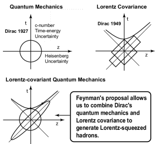
Figure 1: Lorentz-squeezed hadrons. Feynman’s proposal leads us to combine Dirac’s quantum mechanics with c-number time-like excitation dir27 , and his light-cone representation of Lorentz boosts dir45 . Dirac also considered using harmonic oscillators to combine quantum mechanics and special relativity dir45 ; dir63 . It is not difficult to obtain the third figure by combining the first two. The Lorentz boost is a squeeze transformation.

This Gaussian factor determines the space-time localization property of all excited-state wave functions, and its space-time localization property is illustrated in terms of the circle and ellipse in Fig. 1. According to this figure, the Lorentz boost is a squeeze transformation. This figure combines Dirac’s four papers aimed at combining quantum mechanics with special relativity dir49 ; dir27 ; dir45 ; dir63 .

It is important to note that this Lorentz squeeze property has been experimentally verified in various observations in high-energy physics, including Feynman’s parton picture knp86 ; fey69a ; kim89 .

III Squeezed States

Let us start with the Hamiltonian of the form

$$H_{+}=\frac{1}{2}\left\{\left[-\left(\frac{\partial}{\partial x_{1}}\right)^{2}+x_{1}^{2}\right]+\left[-\left(\frac{\partial}{\partial x_{2}}\right)^{2}+x_{2}^{2}\right]\right\},$$ (23)

and the differential equation

$$H_{+}\psi\left(x_{1},x_{2}\right)=\left(n_{1}+n_{2}+1\right)\psi\left(x_{1},x_{2}\right).$$ (24)

This is the Schrödinger equation for the two-dimensional harmonic oscillator. This differential equation is separable in the $x_{1}$ and $x_{2}$ variables, and the wave function can be written as

$$\psi\left(x_{1},x_{2}\right)=\chi_{n_{1}}\left(x_{1}\right)\chi_{n_{2}}\left(x_{2}\right),$$ (25)

where $\chi_{n}(x)$ is the $n$-th excited-state oscillator wave function which takes the form

$$\chi_{n}(x)=\left[\frac{1}{\sqrt{\pi}2^{n}n!}\right]^{1/2}H_{n}(x)\exp{\left(\frac{-x^{2}}{2}\right)}.$$ (26)

Thus

$$\psi\left(x_{1},x_{2}\right)=\left[\frac{1}{\pi 2^{(n_{1}+n_{2})}(n_{1}+n_{2})!}\right]^{1/2}H_{n_{1}}\left(x_{1}\right)H_{n_{2}}\left(x_{2}\right)\exp{\left\{-\frac{1}{2}\left(x_{1}^{2}+x_{2}^{2}\right)\right\}}.$$ (27)

If the system is in the ground state with $n_{1}=n_{2}=0$, this wave function becomes

$$\psi\left(x_{1},x_{2}\right)=\left[\frac{1}{\pi}\right]^{1/2}\exp{\left\{-\frac{1}{2}\left(x_{1}^{2}+x_{2}^{2}\right)\right\}}.$$ (28)

If the $x_{2}$ coordinate alone is in its ground state, the wave function becomes

$$\psi\left(x_{1},x_{2}\right)=\left[\frac{1}{\pi 2^{n}n!}\right]^{1/2}H_{n}\left(x_{1}\right)\exp{\left\{-\frac{1}{2}\left(x_{1}^{2}+x_{2}^{2}\right)\right\}},$$ (29)

with $n=n_{1}$. In order to squeeze this wave function, we introduce first the normal coordinates

$$y_{1}=\frac{1}{\sqrt{2}}\left(x_{1}+x_{2}\right),\qquad y_{2}=\frac{1}{\sqrt{2}}\left(x_{1}-x_{2}\right).$$ (30)

In terms of these variables, the wave function of Eq.(28) can be written as

$$\psi_{0}^{n}(x_{1},x_{2})=\left[\frac{1}{\pi n!2^{n}}\right]^{1/2}H_{n}\left(\frac{y_{1}+y_{2}}{\sqrt{2}}\right)\exp{\left\{-\left(\frac{y_{1}^{2}+y_{2}^{2}}{2}\right)\right\}},$$ (31)

Let us next squeeze the system by making the following coordinate transformation.

$$y_{1}\rightarrow e^{\eta}y_{1},\qquad y_{2}\rightarrow e^{-\eta}y_{1}.$$ (32)

This transformation is equivalent to

$$x_{1}\rightarrow\left[(\cosh\eta)x_{1}+(\sinh\eta)x_{2}\right],\qquad x_{2}\rightarrow\left[(\sinh\eta)x_{1}+(\cosh\eta)x_{2}\right],$$ (33)

like the Lorentz boost given in Eq.(II).

The wave function then becomes

$$\psi_{\eta}^{n}\left(x_{1},x_{2}\right)=\left[\frac{1}{\pi n!2^{n}}\right]^{1/2}H_{n}\left(\frac{e^{-\eta}y_{1}+e^{\eta}y_{2}}{\sqrt{2}}\right)\exp{\left\{-\left[\frac{e^{-2\eta}y_{1}^{2}+e^{2\eta}y_{2}^{2}}{2}\right]\right\}},$$ (34)

If we use the $x_{1}$ and $x_{2}$ variables, this expression becomes

$$\psi_{\eta}^{n}\left(x_{1},x_{2}\right)=\left[\frac{1}{\pi n!2^{n}}\right]^{1/2}H_{n}\left(\frac{e^{-\eta}\left(x_{1}+x_{2}\right)e^{\eta}\left(x_{1}-x_{2}\right)}{2}\right)\exp{\left\{-\left[\frac{e^{-2\eta}\left(x_{1}+x_{2}\right)^{2}+e^{2\eta}\left(x_{1}-x_{2}\right)^{2}}{2}\right]\right\}}.$$ (35)

This transformed wave function does not satisfy the eigenvalue equation of Eq.(24). It is a linear combinations of the eigen solutions $\chi\left(x_{1}\right)$ and $\chi\left(x_{1}\right)$ defined in Eq.(26). The linear expansion takes the form knp86 ; knp91

$$\psi_{\eta}^{n}\left(x_{1},x_{2}\right)=\left(\frac{1}{\cosh\eta}\right)^{(n+1)}\sum_{k}\left[\frac{(n+k)!}{n!k!}\right]^{1/2}(\tanh\eta)^{k}\chi_{n+k}\left(x_{1}\right)\chi_{k}\left(x_{2}\right),$$ (36)

In quantum optics, the eigen functions $\chi_{n+k}\left(x_{1}\right)$ and $\chi_{k}\left(x_{1}\right)$ correspond to the $(n+k)$-photon state of the first photon and $k$-photon state of the second photon respectively.

If $n=0$, it becomes the squeezed ground state or vacuum state, and the resulting wave function is

$$\psi_{\eta}^{0}\left(x_{1},x_{2}\right)=\left(\frac{1}{\cosh\eta}\right)\sum_{k}(\tanh\eta)^{k}\chi_{n+k}\left(x_{1}\right)\chi_{n}\left(x_{2}\right),$$ (37)

In the literature, this squeezed ground state is known as the squeezed vacuum state yuen76 , while the expansion of Eq.(36) is for the squeezed $n$-photon state knp91 .

While these wave functions do not satisfy the eigenvalue equation with the Hamiltonian of Eq.(23), they satisfy the eigenvalue equation with the Hamiltonian $H_{-}$, where

$$H_{-}=\frac{1}{2}\left\{\left[-\left(\frac{\partial}{\partial x_{1}}\right)^{2}+x_{1}^{2}\right]-\left[-\left(\frac{\partial}{\partial x_{2}}\right)^{2}+x_{2}^{2}\right]\right\}.$$ (38)

If the $x_{2}$ coordinate is in its ground state,

$$H_{-}\psi\left(x_{1},x_{2}\right)=n\psi\left(x_{1},x_{2}\right).$$ (39)

If we replace the notations $x_{1}$ and $x_{2}$ by $z$ and $t$ respectively, this Hamiltonian becomes that of Eq.(11). Thus, the oscillator equation of Eq.(11) generates a set of solutions which forms the basis for the squeezed states.

The $t$ variable is the time-separation variable, and is not the time variable appearing in the time-dependent Schrödinger equation. We shall discuss this variable in detail in Sec. IV.

The differential equation of Eq.(11) was proposed by Feynman et al. in 1971 fkr71 . Even though they were not able to provide physically meaningful solutions to their own equation, it is gratifying to note that there is at least one set of solutions which can explain many aspects of physics, including squeezed states in quantum optics as well as the basic observable effects in high-energy hadronic physics.

IV Feynman’s Rest of the Universe

In Sec. II, the time-separation variable played a major role in making the oscillator system Lorentz-covariant. It should exist wherever the space separation exists. The Bohr radius is the measure of the separation between the proton and electron in the hydrogen atom. If this atom moves, the radius picks up the time separation, according to Einstein kn06aip .

On the other hand, the present form of quantum mechanics does not include this time-separation variable. The best way we can do at the present time is to treat this time-separation as a variable in Feynman’s rest of the universe hkn99ajp . In his book on statistical mechanics fey72 , Feynman states

When we solve a quantum-mechanical problem, what we really do is divide the universe into two parts - the system in which we are interested and the rest of the universe. We then usually act as if the system in which we are interested comprised the entire universe. To motivate the use of density matrices, let us see what happens when we include the part of the universe outside the system.

The failure to include what happens outside the system results in an increase of entropy. The entropy is a measure of our ignorance and is computed from the density matrix neu32 . The density matrix is needed when the experimental procedure does not analyze all relevant variables to the maximum extent consistent with quantum mechanics fano57 . If we do not take into account the time-separation variable, the result is therefore an increase in entropy kiwi90pl ; kim07 .

It is gratifying to note that the two-mode coherent state in quantum optics shares the same mathematical basis as the covariant harmonic oscillator. In the two-mode squeezed state, both photons are observable, but the physics survives and becomes even more interesting if one of them is not observed ekn89 .

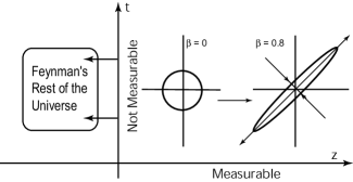
Figure 2: Localization property in the $zt$ plane. When the hadron is at rest, the Gaussian form is concentrated within a circular region specified by $(z+t)^{2}+(z-t)^{2}=1.$ As the hadron gains speed, the region becomes squeezed to $e^{-2\eta}(z+t)^{2}+e^{2\eta}(z-t)^{2}=1.$ Since it is not possible to make measurements along the $t$ direction, we have to deal with the information less than complete, and to resort to entropy.

In the covariant oscillator formalism, these two photons are translated into longitudinal and time-like excitations in the hadronic system. If the hadron is at rest, there are no time-like excitations. On the other hand, if the hadron moves, there are time-like excitations to the observer at rest. But this observer is not able to detect it. Indeed, these time-like oscillations are in Feynman’s rest of the universe.

Let us carry out a concrete mathematics using the density matrix formalism. From the covariant oscillator wave functions defined Sec. II, the pure-state density matrix is

$$\rho_{\eta}^{n}(z,t;z^{\prime},t^{\prime})=\psi_{\eta}^{n}(z,t)\psi_{\eta}^{n}(z^{\prime},t^{\prime}),$$ (40)

which satisfies the condition $\rho^{2}=\rho:$

$$\rho_{\eta}^{n}(z,t;x^{\prime},t^{\prime})=\int\rho_{\eta}^{n}(z,t;x",t")\rho_{\eta}^{n}(z",t";z^{\prime},t^{\prime})dz"dt".$$ (41)

However, in the present form of quantum mechanics, it is not possible to take into account the time separation variables. Thus, we have to take the trace of the matrix with respect to the t variable. Then the resulting density matrix is kiwi90pl

$$\rho_{\eta}^{n}(z,z^{\prime})=\int\psi_{\eta}^{n}(z,t)\psi_{\eta}^{n}(z^{\prime},t)dt$$

$$\hskip 42.67912pt=\left(\frac{1}{\cosh\eta}\right)^{2(n+1)}\sum_{k}\frac{(n+k)!}{n!k!}(\tanh\eta)^{2k}\psi_{n+k}(z)\psi^{*}_{k+n}(z^{\prime}).$$ (42)

The trace of this density matrix is one, but the trace of $\rho^{2}$ is less than one, as we can see from the following formula.

$$Tr\left(\rho^{2}\right)=\int\rho_{\eta}^{n}(z,z^{\prime})\rho_{\eta}^{n}(z^{\prime},z)dzdz^{\prime}$$

$$\hskip 42.67912pt=\left(\frac{1}{\cosh\eta}\right)^{4(n+1)}\sum_{k}\left[\frac{(n+k)!}{n!k!}\right]^{2}(\tanh\eta)^{4k}.$$ (43)

which is less than one. This is due to the fact that we do not know how to deal with the time-like separation in the present formulation of quantum mechanics. Our knowledge is less than complete.

The standard way to measure this ignorance is to calculate the entropy defined as

$$S=-Tr\left(\rho\ln(\rho)\right).$$ (44)

If we can measure the distribution along the time-like direction and use the pure-state density matrix given in Eq.(40), the entropy is zero. However, if we do not know how to deal with the distribution along $t$, then we should use the density matrix of Eq.(IV) to calculate the entropy, and the result is kiwi90pl

$$S=2(n+1)\left\{(\cosh\eta)^{2}\ln(\cosh\eta)-(\sinh\eta)^{2}\ln(\sinh\eta)\right\}-\left(\frac{1}{\cosh\eta}\right)^{2(n+1)}\sum_{k}\frac{(n+k)!}{n!k!}\ln\left[\frac{(n+k)!}{n!k!}\right](\tanh\eta)^{2k}.$$ (45)

In terms of the velocity $v$ of the hadron,

$$S=-(n+1)\left\{\ln\left[1-\left(\frac{v}{c}\right)^{2}\right]+\frac{(v/c)^{2}\ln(v/c)^{2}}{1-(v/c)^{2}}\right\}-\left[1-\left(\frac{1}{v}\right)^{2}\right]\sum_{k}\frac{(n+k)!}{n!k!}\ln\left[\frac{(n+k)!}{n!k!}\right]\left(\frac{v}{c}\right)^{2k}.$$ (46)

Let us go back to the wave function given in Eq.(20). As is illustrated in Figure 1, its localization property is dictated by the Gaussian factor which corresponds to the ground-state wave function. For this reason, we expect that much of the behavior of the density matrix or the entropy for the $n$-th excited state will be the same as that for the ground state with $n=0.$ For this state, the density matrix and the entropy are

$$\rho(z,z^{\prime})=\left(\frac{1}{\pi\cosh(2\eta)}\right)^{1/2}\exp{\left\{-\frac{1}{4}\left[\frac{(z+z^{\prime})^{2}}{\cosh(2\eta)}+(z-z^{\prime})^{2}\cosh(2\eta)\right]\right\}},$$ (47)

and

$$S=2\left\{(\cosh\eta)^{2}\ln(\cosh\eta)-(\sinh\eta)^{2}\ln(\sinh\eta)\right\},$$ (48)

respectively. The quark distribution $\rho(z,z)$ becomes

$$\rho(z,z)=\left(\frac{1}{\pi\cosh(2\eta)}\right)^{1/2}\exp{\left(\frac{-z^{2}}{\cosh(2\eta)}\right)}.$$ (49)

The width of the distribution becomes $\sqrt{\cosh\eta}$, and becomes wide-spread as the hadronic speed increases. Likewise, the momentum distribution becomes wide-spread knp86 ; hkn90pl . This simultaneous increase in the momentum and position distribution widths is called the parton phenomenon in high-energy physics fey69a . The position-momentum uncertainty becomes $\cosh\eta$. This increase in uncertainty is due to our ignorance about the physical but unmeasurable time-separation variable.

Let us next examine how this ignorance will lead to the concept of temperature. For the Lorentz-boosted ground state with $n=0$, the density matrix of Eq.(47) becomes that of the harmonic oscillator in a thermal equilibrium state if $(\tanh\eta)^{2}$ is identified as the Boltzmann factor hkn90pl . For other states, it is very difficult, if not impossible, to describe them and thermal equilibrium states. Unlike the case of temperature, the entropy is clearly defined for all values of $n$. Indeed, the entropy in this case is derivable directly from the hadronic speed.

The time-separation variable exists in the Lorentz-covariant world, but we pretend not to know about it. It thus is in Feynman’s rest of the universe. If we do not measure this time-separation, it becomes translated into the entropy.

CONCLUSIONS

In this paper, we started with the Lorentz-invariant differential equation of Feynman et al. fkr71 . This equation can be separated into the Klein-Gordon equation for the free-flying hadron and the harmonic-oscillator equation for the quarks inside the hadron. It was noted that there is a set of solutions constituting a representation of the Poincaré group knp86 . While this set leads to many interesting consequences in high-energy physics, it serves as the mathematical basis for squeezed states in quantum optics. This also serves as a mathematical tool for illustrating Feynman’s rest of the universe.

Starting from the physics of two-mode squeezed states, we were able to give a physical interpretation to the time-separation variable which is never mentioned in the present form of quantum mechanics.

According to Feynman, the adventure of our science of physics is a perpetual attempt to recognize that the different aspects of nature are really different aspects of the same thing. While this is his interpretation of physics, the question is how to accomplish it. One way is to prove that everything in physics comes from one equation, as Newton did for classical mechanics. Feynman’s equation of Eq.(1) does not appear to generate all the physics, but it could serve as the starting point in many branches of physics.

References

- (1) F. J. Dyson, Physics Today, June, 21 (1965).
- (2) Y. S. Kim, Phys. Rev. 142, 1150 (1966).
- (3) R. P. Feynman, M. Kislinger, and F. Ravndal, Phys. Rev. D 3, 2706 (1971).
- (4) E. Wigner, Ann. Math. 40, 149 (1939).
- (5) Y. S. Kim, M. E. Noz, and S. H. Oh, J. Math. Phys. 20, 1341 (1979).
- (6) H. P. Yuen, Phys. Rev. A 13, 2226 (1976).
- (7) A. K. Ekert and P. L. Knight, Am. J. Phys. 57, 692 (1989).
- (8) Y. S. Kim and M. E. Noz, Theory and Applications of the Poincaré Group (Reidel, Dordrecht, 1986).
- (9) P. A. M. Dirac, Rev. Mod. Phys. 21, 392–399 (1949).
- (10) P. A. M. Dirac, Proc. Roy. Soc. (London) A114, 243 (1927).
- (11) P. A. M. Dirac, Proc. Roy. Soc. (London) A183, 284 (1945).
- (12) P. A. M. Dirac, J. Math. Phys. 4, 901-909 (1963).
- (13) R. P. Feynman, Phys. Rev. Lett. 23, 1415-1417 (1969).
- (14) Y. S. Kim, Phys. Rev. Lett. 63, 348 (1989).
- (15) Y. S. Kim and M. E. Noz, Phase Space Picture of Quantum Mechanics (World Scientific, Singapore, 1991).
- (16) Y. S. Kim and M. E. Noz, 2006 The Question of Simultaneity in Relativity and Quantum Mechanics. in QUANTUM THEORY: Reconsideration of Foundations - 3 (ed. G. Adenier, A. Khrennikov, and T. M. Nieuwenhuizen), AIP Conference Proceedings 180, pp. 168-178 (American Institute of Physics 2006).
- (17) D. Han, Y. S. Kim, and E. E. Noz, Am. J. Phys. 67, 61 (1999).
- (18) R. P. Feynman, Statistical Mechanics (Benjamin/Cummings, Reading, Massachusetts, 1972).
- (19) J. von Neumann, Die mathematische Grundlagen der Quanten-mechanik (Springer, Berlin, 1932). See also J. von Neumann, Mathematical Foundation of Quantum Mechanics (Princeton University, Princeton, 1955).
- (20) U. Fano, Rev. Mod. Phys. 29, 74-93 (1957).
- (21) Y. S. Kim and E. P. Wigner, Phys. Lett. A 147, 343 (1990).
- (22) Y. S. Kim, Coupled oscillators and Feynman’s three papers, J. Phys. Conf. Ser. 70, 012010 (2007).
- (23) D. Han, Y. S. Kim, and M. E. Noz, Phys. Lett. A 144, 111 (1990).