Star Clusters in Pseudo-bulges of Spiral Galaxies

Abstract

We present a study of the properties of the star-cluster systems around pseudo-bulges of late-type spiral galaxies using a sample of 11 galaxies with distances from 17 to 37 Mpc. Star clusters are identified from multiband HST ACS and WFPC2 imaging data by combining detections in 3 bands (F435W and F814W with ACS and F606W with WFPC2). The photometric data are then compared to population synthesis models to infer the masses and ages of the star clusters. Photometric errors and completeness are estimated by means of artificial source Monte Carlo simulations. Dust extinction is estimated by considering F160W NICMOS observations of the central regions of the galaxies, augmenting our wavelength coverage. In all galaxies we identify star clusters with a wide range of ages, from young (age $\lesssim$ 8 Myr) blue clusters, with typical mass of $10^{3}$ ${\mathrm{M}_{\sun}}$ to older (age $>$ 100-250 Myr), more massive, red clusters. Some of the latter might likely evolve into objects similar to the Milky Way’s globular clusters. We compute the specific frequencies for the older clusters with respect to the galaxy and bulge luminosities. Specific frequencies relative to the galaxy light appear consistent with the globular cluster specific frequencies of early-type spirals. We compare the specific frequencies relative to the bulge light with the globular cluster specific frequencies of dwarf galaxies, which have a surface-brightness profile that is similar to that of the pseudo-bulges in our sample. The specific frequencies we derive for our sample galaxies are higher than those of the dwarf galaxies, supporting an evolutionary scenario in which some of the dwarf galaxies might be the remnants of harassed late-type spiral galaxies which hosted a pseudo-bulge.

1 Introduction

Over the last two decades, observational evidence has been accumulating that not all spiral galaxies possess a bulge resembling a small elliptical galaxy with a de Vaucouleurs R^1/4 light profile. Bulges with a surface-brightness profile that does not follow the de Vaucouleurs law also show disk-like, cold stellar kinematics (Kormendy, 1993) and light profiles that are well-fitted by an exponential or an intermediate Sersic law (Andredakis et al., 1995). For these reasons these bulges are known as pseudo-bulges or exponential bulges. HST imaging of pseudo-bulges has also revealed that they often contain central compact sources, most likely star clusters (Carollo et al., 1998) and that they have shallower nuclear slopes than traditional bulges with the same magnitude (Carollo & Stiavelli, 1998). It is also intriguing that the nuclear cusp slopes of the exponential bulges are similar to those of dwarf elliptical galaxies with the same radii and luminosities. This similarity suggests that there might be an evolutionary link between pseudo-bulges and dwarf ellipticals, as if the presence of a disk did not affect the nuclear properties of pseudo-bulge spirals (Stiavelli et al., 2001).

In order to study in detail the properties of pseudo-bulges and investigate possible formation scenarios, we isolated a sample of 11 pseudo-bulges from our previous HST surveys with WFPC2 and NICMOS and obtained for this sample additional HST/ACS imaging data. The relation between bulge properties and galaxy properties for these systems has been discussed already by Carollo et al. (2007). These authors found that the bulge properties correlate very well with those of the host galaxy, suggesting that evolutionary processes of the disk may be responsible for the formation of the pseudo-bulges. In this paper we focus rather on the properties of the population of star clusters within the pseudo-bulges.

We have two main goals. The first is to characterize the star-cluster systems of these late-type pseudo-bulge hosts and to compare them with the growing body of literature focused on spirals with classical bulges (for a review see Brodie & Strader 2006). Under the assumption that globular clusters form in association with enhanced bursts of star formation (e.g. Beasley et al. 2002), the abundance of globular clusters is expected to depend on whether a bulge is formed “classically”, that is with a single burst of star formation, or more slowly, through extended star formation associated with secular processes in the quiescent galaxy disk (Kormendy & Kennicutt, 2004; Brodie & Strader, 2006). In this latter scenario, a lower specific frequency would be expected.

The second goal is to continue to investigate the similarities between pseudo-bulges and dwarf ellipticals, first highlighted by Stiavelli et al. (2001). A spiral galaxy can be stripped of its disk during close interactions with neighbors, especially effective in a group environment (Moore et al., 1996). This “galaxy harassment” scenario suggests evolution of late-type spirals with a pseudo-bulge into dwarf ellipticals. The stellar populations of low-mass galaxies in clusters are indeed consistent with some fraction having evolved in this manner (e.g. Conselice, Gallagher & Wyse 2003). Under this scenario, there should also be a correlation between the properties of the star-cluster systems of these two galaxy classes. Here we explore this connection by measuring the specific frequencies of globular clusters per bulge light in our sample and comparing it with those of dwarf ellipticals.

This paper is organized as follows. We briefly introduce the sample and discuss the data reduction in Section 2. Source detection and photometry are described in Section 3. Star clusters are identified in Section 4 based on a color and luminosity selection. Systematic uncertainties are discussed in Section 5. Specific frequencies for the star cluster systems are derived in Section 6 while Section 7 briefly illustrates the properties of nuclear star clusters. Our interpretation and conclusions are discussed in Section 8.

2 Sample and Data Reduction

We use images of 11 late-type spiral galaxies obtained during the HST-ACS pseudo-bulge survey GO-9395 (PI: C. M. Carollo). The same systems were also observed previously with WFPC2 and NICMOS (Carollo et al., 1997, 1998; Carollo & Stiavelli, 1998). All galaxies were selected on the basis of: (1) angular diameter larger than 1′; (2) regular morphological type; (3) redshift less than 2500 km s^-1, to guarantee a high angular resolution in physical size; and (4) an inclination angle, estimated from the apparent axial ratio, smaller than 75°, to avoid strong obscuration of the nucleus by the disk. The objects of this study had also be shown to possess an exponential bulge (Carollo & Stiavelli, 1998; Carollo et al., 2007). The galaxy coordinates, distance (assuming $H_{0}=73$ km s^-1 Mpc^-1 for the Hubble constant), absolute magnitude, morphological classification and galactic extinction are listed in Table 1. For each galaxy, we have ACS/WFC images in the F435W and F814W filters, WFPC2 images in the F606W filter and NICMOS images in the F160W filter.

The exposures in the F606W ($V$) filter were acquired between 1996 and 1997 by WFPC2 with the galaxy nucleus centered on the PC camera (the only WFPC2 chip considered in this study as its resolution is comparable with ACS/WFC), which has a scale of 0.046″ pixel^-1 and a field of view of about 35″x 35″. The observations were carried out in fine lock with a nominal gain of 15 electrons/DN and a total exposure time per field of 600 s, split in two to allow removal of cosmic rays. For these images the raw data were processed with the standard WFPC2 pipeline (CALWP2) in order to use the most recent reference frames for flat-fielding, bias and dark current subtractions; the cosmic-rays were removed using the IRAF STSDAS task CRREJ and the remaining hot pixels were removed by interpolation. Finally, sky subtraction was performed by determining the sky values from the WF chips, in areas farthest from the nucleus.

The images in the F435W ($B$) and F814W ($I$) filters were acquired between 2002 and 2003. The observations were carried out with the ACS/WFC channel, whose pixel scale is 0.05″ pixel^-1 for a total field of view of 3.4′x 3.4′. Details of these observations can be found in Carollo et al. (2007). The standard ACS pipeline (CALACS) was used to perform the basic data reduction (flat-fielding, bias and dark subtractions and removal of the overscan regions), then the IRAF STSDAS tasks ACSREJ and DRIZZLE were used, respectively, to achieve cosmic-ray rejection and to correct for geometric distortions. Finally, any remaining hot pixels were removed by interpolation and sky subtraction was carried out for all galaxies.

The images in the F160W ($H$) filter were acquired between 1997 and 1998 by NICMOS (Camera 2). The pixel scale is 0.075″ pixel^-1 for a total field of view of about 19.2″x 19.2″. These observations were carried out in snapshot mode and split into multiple exposures (to allow better cosmic-ray rejection) for a total exposure time per field of 384 s for ESO 498G5, ESO 499G37, NGC 1345, NGC 1483, NGC 3259 and NGC2758 and a total exposure time per field of 256 s for NGC 406, NGC 2082, NGC 3455, NGC4980 and NGC 6384. These images were reduced through the standard pipeline software (CALNICA). The various NICMOS anomalies (e.g. the pedestal anomaly) were corrected on a case-by-case basis. We direct the reader to Carollo et al. (2002) for further details.

3 Photometry

3.1 Source Detections & Aperture Photometry

Our goal is to identify star-cluster candidates and to characterize their integrated photometric properties. Therefore we aim at constructing a uniform catalog of sources, focusing on detections that lie in the common area of the F435W, F606W and F814W images. The resulting search radius for each galaxy is given in the last column of Table 1. The NICMOS F160W images have a more limited field of view and we use them only to evaluate the possible impact of dust extinction (see Section 5.1).

Our study is limited to star clusters close to the nucleus of the host galaxy, where there are significant inhomogeneities in the image background, mainly due to dust lanes and gradients in the integrated-light profile. Therefore, we identify star-cluster candidates on a ‘variance-normalized’ image, that allows improved detection of point-like sources in regions of rapidly varying background (Miller et al., 1997). The ‘variance-normalized’ image is obtained by summing the F435W and F814W images to improve the signal to noise ratio and then by dividing the result by a smoothed version of itself, realized with a 11x11 pixel median filter.

We use the IRAF task DAOFIND to search for star clusters in the images. This task, optimized for point-source detection, is adequate for our goal, due to the compact size (FWHM $\approx$ 1 or 2 pixels) of the star clusters in our sample. Indeed, for our purposes, with our data, DAOFIND marginally outperforms extended-source detection packages such as SExtractor (Bertin & Arnouts, 1996).

The coordinates of the sources detected on the ‘variance-normalized’ image are then mapped into the local pixel coordinates of each image using the IRAF tasks XY2RD, RD2XY and GEOMAP. We visually inspected all sources, with particular attention paid to those with FWHM $>0.25\arcsec$ in the F435W band, corresponding to a half-light radius $R=0.15\arcsec$ after deconvolution with the PSF, if the source has a Plummer surface brightness profile (see Section 3.2). The angular scale $R=0.15\arcsec$ corresponds to R $\approx$ 13 pc at 17 Mpc — the distance of our closest galaxy — and R $\approx$ 27 pc at 38 Mpc — the distance of the farthest galaxy. These more extended sources have in general very low surface brightness and often appear to be artifacts and are thus excluded from the subsequent analysis. This cut is primarily motivated by the size distribution of galactic GCs, which have radii smaller than about 20 pc. In addition, all the sources in our final catalog have been visually inspected to remove bright foreground stars identified from their diffraction spikes.

We perform circular aperture photometry of all the detected sources using an aperture radius of 0.15″ for each image and estimating the background level in an annulus between 0.5″ and 1″ in radius. We verify that this method yields a correct estimate of the background including the galaxy luminosity. We checked this by choosing the central part of the galaxies, where their luminosity gradient is steepest and comparing our photometry of the nuclear star clusters against the published photometry of Carollo et al. (1997, 1998), which took into account a detailed model of the galaxy light profile. In addition, the aperture correction and error estimates have been performed via Monte Carlo simulations on the actual images (see Section 3.2), therefore any residual bias is corrected to first order.

We consider only sources that in all bands have a magnitude greater than a chosen threshold magnitude, corresponding to a signal-to-noise ratio (SNR) greater than 5 (see Table 2). The photometric calibration is done by converting instrumental magnitudes to the VEGAMAG magnitude system by applying the photometric zeropoints listed in Table 2. All magnitudes are then corrected for Galactic extinction following Schlegel et al. (1998). Since the HST filters differ from the Johnson-Cousins band-passes, reddening corrections are computed using the effective transmission curve for each HST filter, created with the IRAF task CALCBAND in the SYNPHOT package (see Table 2).

In this paper we indicate with uppercase letters (e.g. $V$) the apparent magnitude in the HST filters, while we use symbols like $M_{V}$ for the corresponding absolute magnitude. Absolute magnitudes in Johnson-Cousins bands are instead indicated with symbols like $M_{V_{JC}}$.

3.2 Aperture Correction & Uncertainty Estimates

Total magnitudes are determined by correcting for flux outside the measurement aperture. Aperture corrections, photometric uncertainties and the completeness of our observations are estimated by means of Monte Carlo simulations. We add artificial star clusters of known luminosity and size to each image in random positions within the search area defined in Section 3.1 and we measure the retrieved flux with the same aperture photometry procedure adopted for the real sources. The luminosity profile of the simulated star clusters follows a projected Plummer law:

$$L(R)=\frac{L_{tot}}{\pi b^{2}}\left(1+\frac{R^{2}}{b^{2}}\right)^{-2}$$ (1)

where $b$ is the assigned scale length and $L$ is the assigned total luminosity. This is then convolved with the Point Spread Function (PSF) in the appropriate filter obtained with TinyTim (Krist & Hook, 2001) before being added to the image.

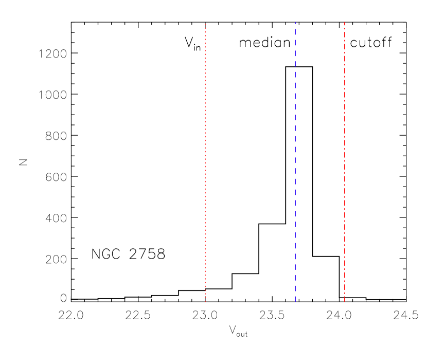
Figure 1: Distribution of retrieved magnitudes ($V_{out}$) obtained through a Monte Carlo simulation with $V_{in}=23$ mag (red dotted line) for the NGC 2758 galaxy in the $V$-band. The resulting median value of the distribution is also shown (blue dashed line). Sources with retrieved magnitude brighter than the $2\sigma$ cutoff (red dot-dashed line) and fainter than $V_{in}$ (red dotted line) are defined as successfully recovered.

The result for a representative photometric Monte Carlo simulation is shown in Fig. 1. Note that the distribution of the output magnitude ($m_{out}$) at a fixed input magnitude ($m_{in}$) has a width much smaller than the difference $m_{out}-m_{in}$. We define the aperture correction as the difference between $m_{in}$ and the median of the distribution of the output magnitude $m_{out}$. We find that the aperture correction is almost independent of $m_{in}$, and depends mildly on the size of the artificial source, with variations of about 0.2 mag for clusters with observed half-light radii between $0.05\arcsec$ and $0.15\arcsec$. We therefore apply the aperture correction to the observed sources according to their apparent size, using linear interpolation across our grid of models.

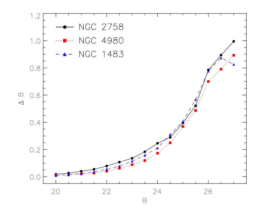
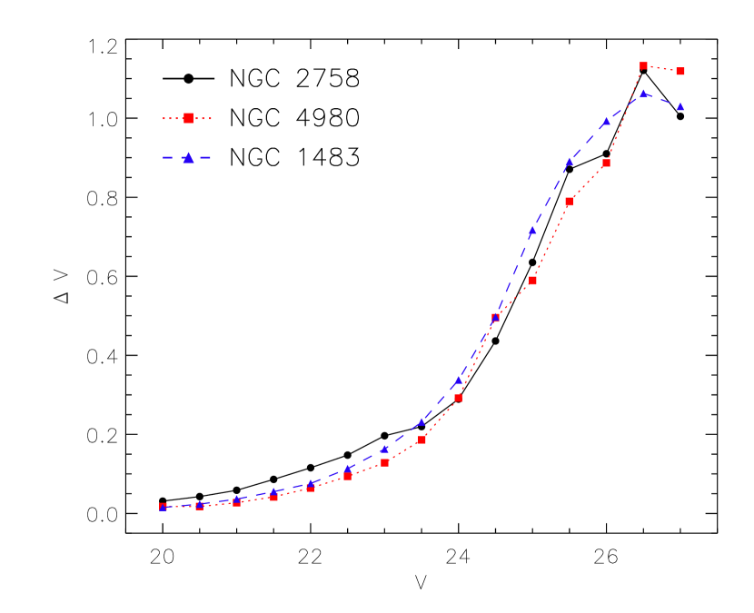
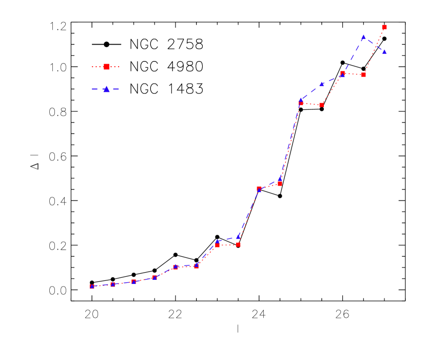
Figure 2: Photometric uncertainties for star cluster-like sources in three galaxies representative of our sample (NGC 2758 solid line, NGC 4980 dotted line and NGC 1483 dashed line). These uncertainties have been estimated via Monte Carlo simulations by placing and recovering artificial sources in the original images.

The error on the photometry is similarly estimated from the Monte Carlo simulations as the variance of the output magnitudes of the artificial sources. The typical uncertainties are plotted in Fig. 2 as a function of the magnitude for three galaxies representative of our sample, NGC 1483 ($D=17.1$ Mpc), NGC 4980 ($D=23.9$ Mpc) and NGC 2758 ($D=31.3$ Mpc). Note that the photometric error so obtained is larger than the formal statistical photometric error reported by the IRAF aperture photometry task.

We neglect the effect of possible varying charge transfer efficiency (CTE) because the observations were carried out when the instruments were still young, thus the effect is not severe. Further, the background levels in the images are provided by the underlying galaxies, rather than just the sky, and are high enough to make the effect minimal (Holtzman et al., 1995).

The errors on the colors are also quantified using our Monte Carlo simulations. We place and recover artificial sources with a given input color ($M_{B}-M_{I}\equiv B-I=1,1.5,2$; $M_{V}-M_{I}$ $\equiv V-I=0,0.5,1;M_{B}-M_{V}\equiv B-V=0,0.5,1$) on the corresponding images. From the recovered photometry we measure the error on the color and correlate it with the errors in each band, under the assumption of a linear relation. For example, in case of the $B-I$ color the error-relation reads:

$$\sigma_{B-I}^{2}=\sigma_{B}^{2}+\sigma_{I}^{2}-2\cdot r_{BI}\cdot\sigma_{B}\cdot\sigma_{I}$$ (2)

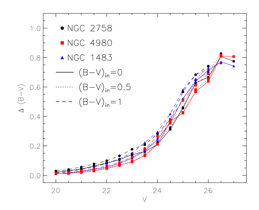
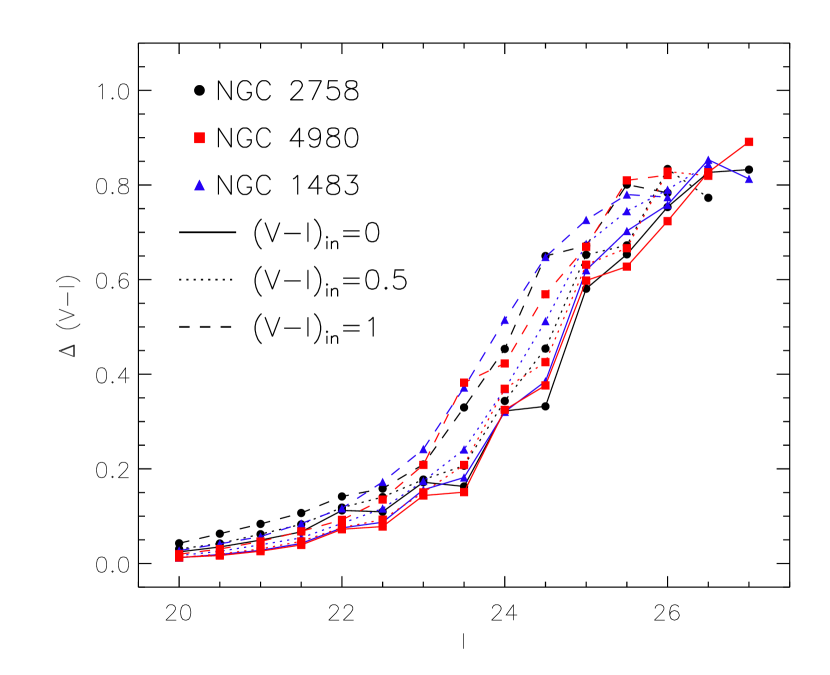
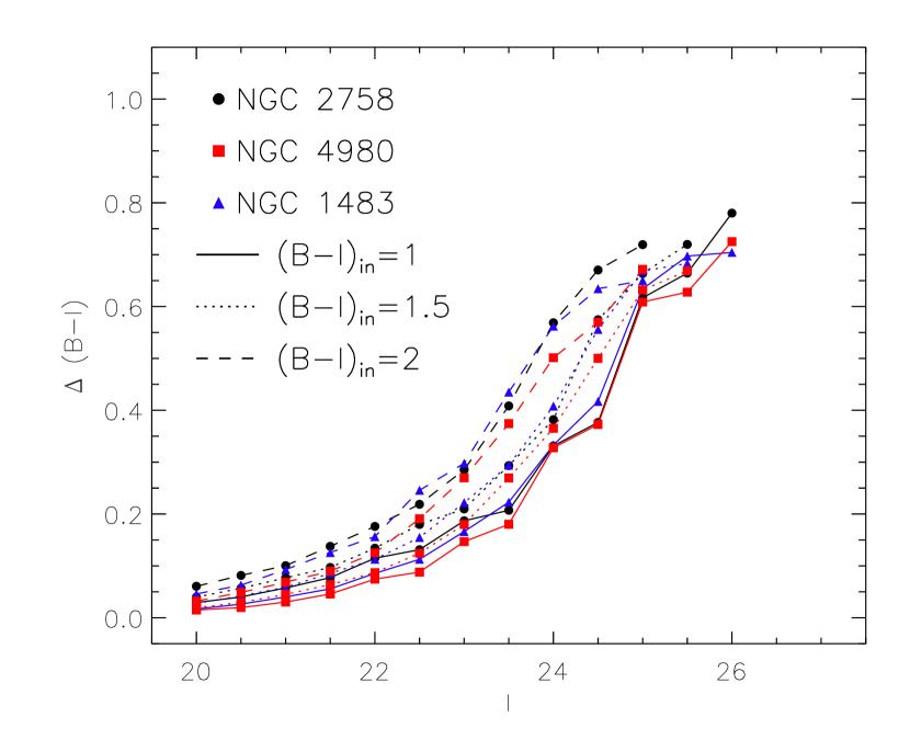
Figure 3: Photometric uncertainties in the color measurements relative to input magnitudes for representative input colors and galaxies in the sample, estimated from Monte Carlo simulations as in Fig. 2.

where $r_{BI}$ is the linear correlation term. The typical uncertainties on the colors are plotted in Fig. 3 as a function of the magnitude and the color itself for the three reference galaxies introduced above. Our analysis yields that the typical value of the correlation $r$ is only mildly dependent on the color itself, with variations from $r\approx 0.5$ to $r\approx 0.9$. We assume a reference value of $r\approx 0.7$ (the average value of the sample), which turns out to describe the color errors satisfactorily.

Finally, through the same Monte Carlo simulations we also determine the completeness of our observations. For this purpose we define as ‘successfully recovered’ a synthetic source whose output magnitude satisfies:

$$m_{in}<m_{out}<m_{in}+m_{corr}+2\sigma$$ (3)

where $m_{in}$ is the assigned input magnitude and $m_{corr}$ and $\sigma$ are respectively the aperture correction and the one-sigma photometric error previously estimated. Note that (i) $m_{corr}>>\sigma$ (for example, see Fig. 1), thus a source which is recovered as brighter than its input luminosity has an error at several standard deviations (essentially this happens only when a synthetic source falls on top of another existing source), which implies failure in the recovery; (ii) the error distribution is highly skewed (see Fig. 1). Thus the completeness is similar if we were to change the cutoff in Eq. 3 to either $1\sigma$ or $3\sigma$.

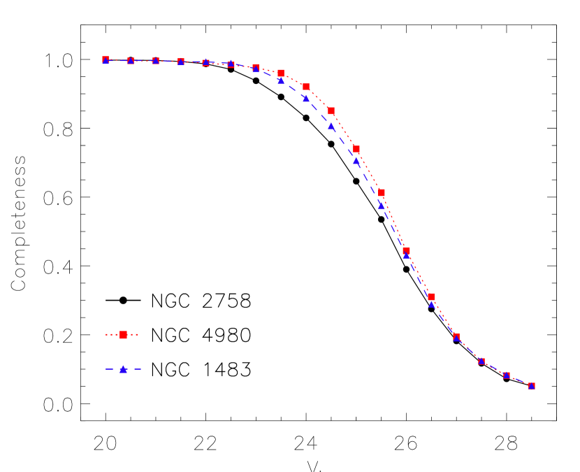
Figure 4: Completeness curves for our survey, determined via Monte Carlo simulations by placing and recovering artificial star-cluster sources with a Plummer surface brightness profile and half-light radius of $0.075\arcsec$, which corresponds to the mean size of the stellar clusters in our sample.

Since we found that the completeness does not significantly depend on the radius of the objects, we show in Fig. 4 only the completeness curves derived for the mean size of the stellar clusters ($0.075\arcsec$) for three galaxies representative of our sample and we note that in all cases the incompleteness becomes severe only at $V>25.5$.

4 Identification of star clusters

To classify star clusters, we compare the colors of the sources in the final catalog with those expected from synthetic stellar populations. For this we use the spectral energy distribution of Bruzual & Charlot (2003) models based on the Padova (1994) tracks, a Salpeter (1955) initial mass function (IMF) with masses between 0.1 and 100 $\mathrm{M_{\sun}}$, a range of metallicities from 0.02 to 1 $\mathrm{Z_{\sun}}$ and ages from 1 Myr to 15 Gyr. In addition we have also included self-consistently Hydrogen and Helium recombination lines as well as metal lines, as described in Oesch et al. (2007). The integrated model colors for the HST filters of the observations have been obtained by processing the synthetic spectra through the IRAF task CALCBAND within the SYNPHOT package. With the CALCBAND task we also include optional dust extinction ($E(B-V)\leqslant 1$ mag). For comparison we also created Bruzual & Charlot (2003) models using a Chabrier (2003) IMF with the same mass cutoffs. As expected, we verified that the resulting optical colors are identical in both cases (in fact the two IMFs are different only for stars below $1~{}\mathrm{M_{\sun}}$). The mass-to-light ratio is a factor $\approx 1.8$ smaller (with very low dependence on age and metallicity) when using a Chabrier IMF instead of a Salpeter IMF, due to the lower fraction of low-mass stars.

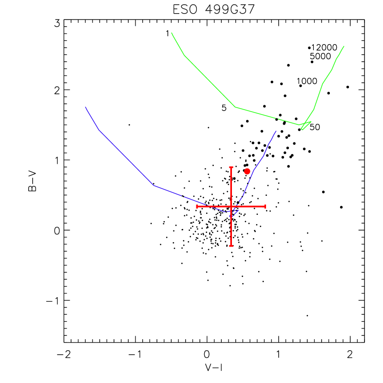
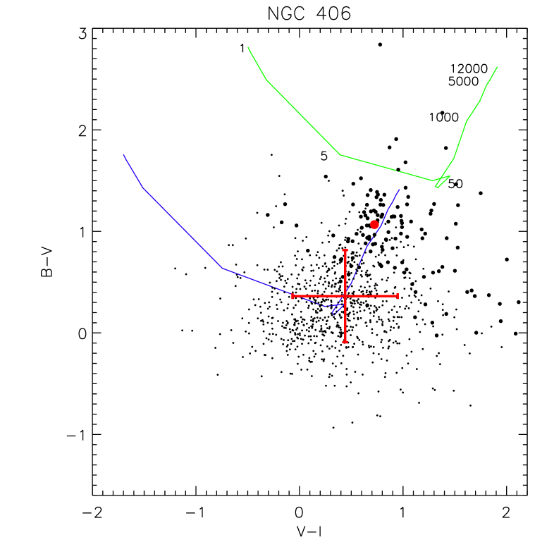
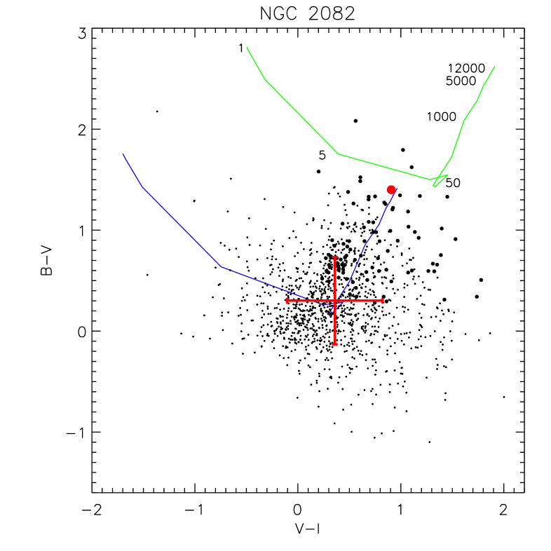
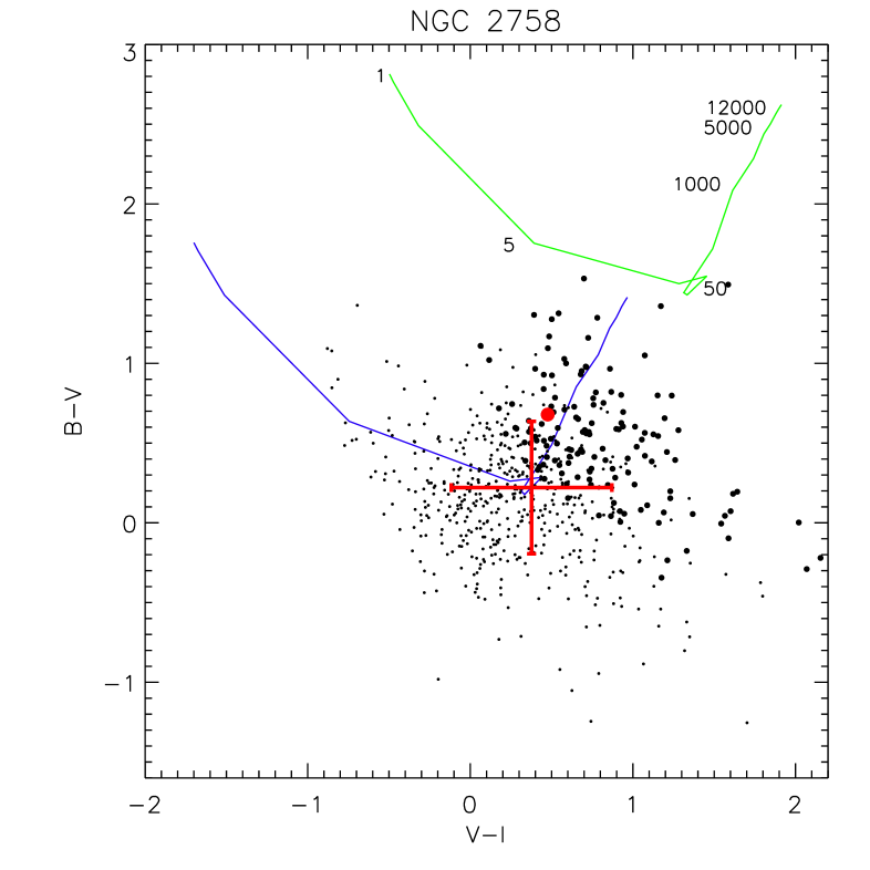
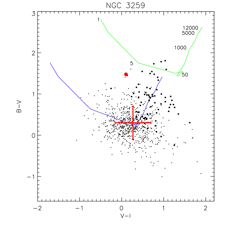
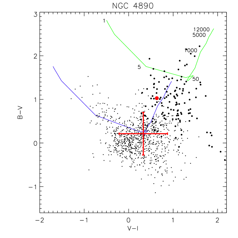
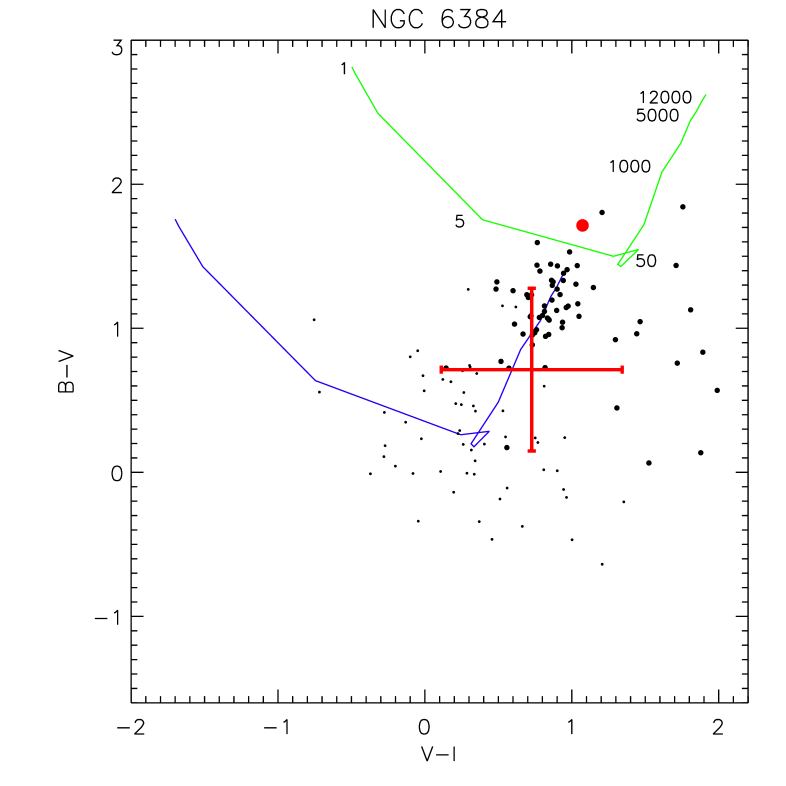
Figure 5: Color-color diagrams ($B-V$ vs. $V-I$) for star clusters in each galaxy, showing a comparison of our data to Bruzual & Charlot (2003) models. Black dots are the data with the “old” (age $\geqslant 250$ Myr) and massive (mass $\geqslant 10^{5}$ $\mathrm{M_{\sun}}$) clusters highlighted in bold. The large red dot corresponds to the nuclear star cluster of each galaxy. The models include emission lines and have solar metallicity, single stellar population, a Salpeter (1955) IMF and no reddening [$E(B-V)=0$, blue line] or a 1 mag of reddening [$E(B-V)=1$, green line]. Along the theoretical tracks we mark the age of the synthetic population in Myr. The star cluster average colors with their $1\sigma$ dispersions are shown in red.

The Salpeter-IMF tracks in the $V-I$ vs. $B-V$ color-color plane are shown in Fig. 5 and compared with the observed sources. Based on these colors, most of the detected sources are consistent with being relatively young star clusters (age $\approx$ 50 Myr). The data-model comparison for all galaxies, except NGC 6384, suggests that only a modest extinction is present (but see section 5.1 for a more detailed discussion). The spread of the observed sources in the color-color plane (standard deviation and central point of the distribution reported in Fig. 5) is comparable with the photometric errors on the colors (see Fig. 3). Hence it is not possible to infer the star-cluster formation history from this plot.

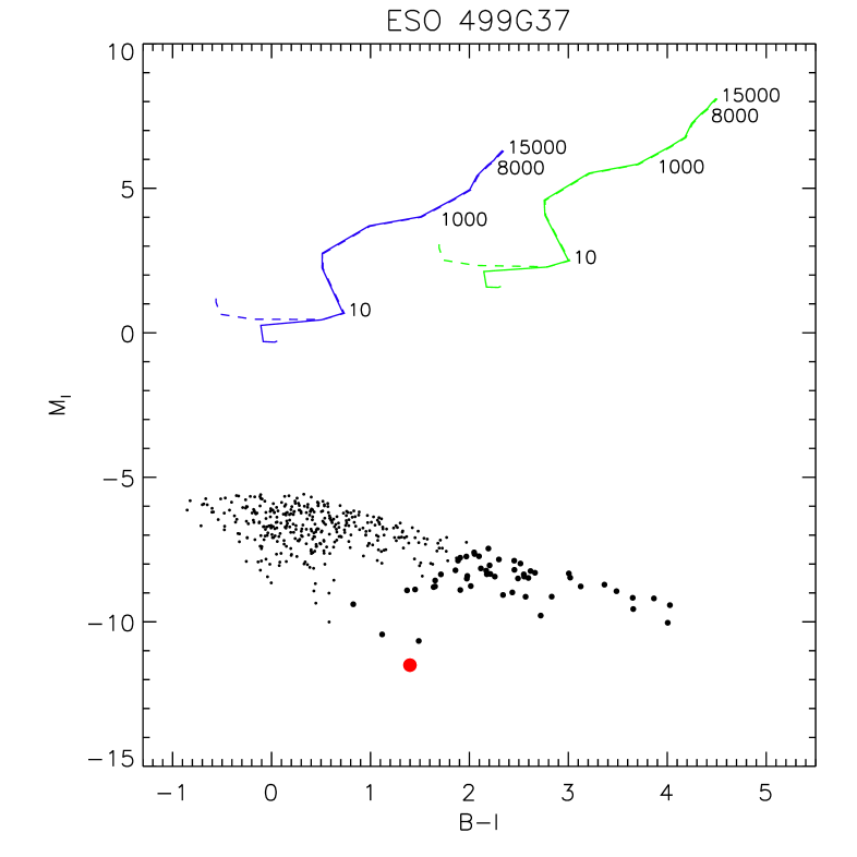
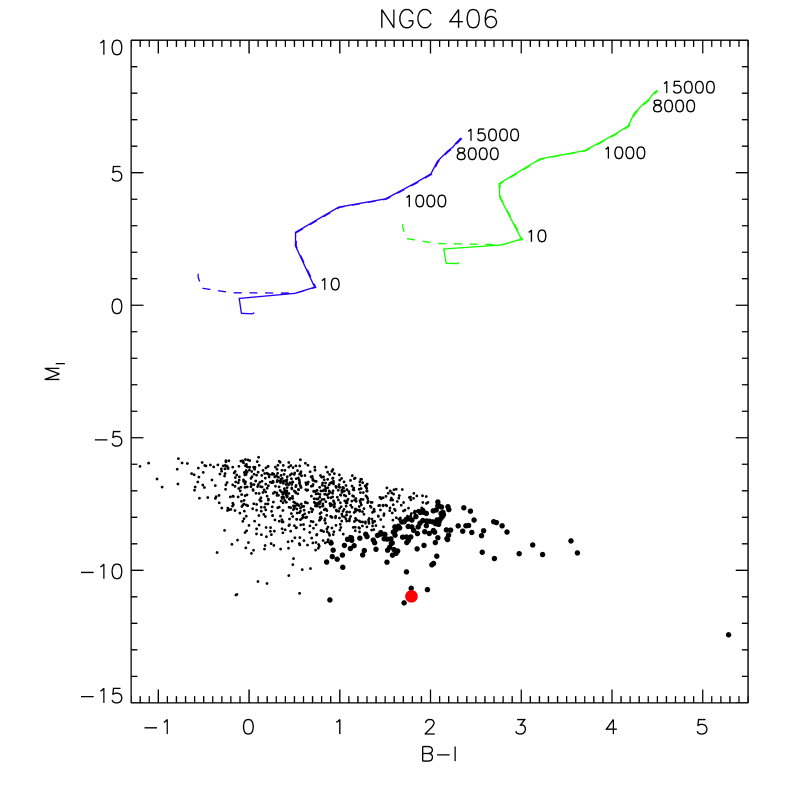
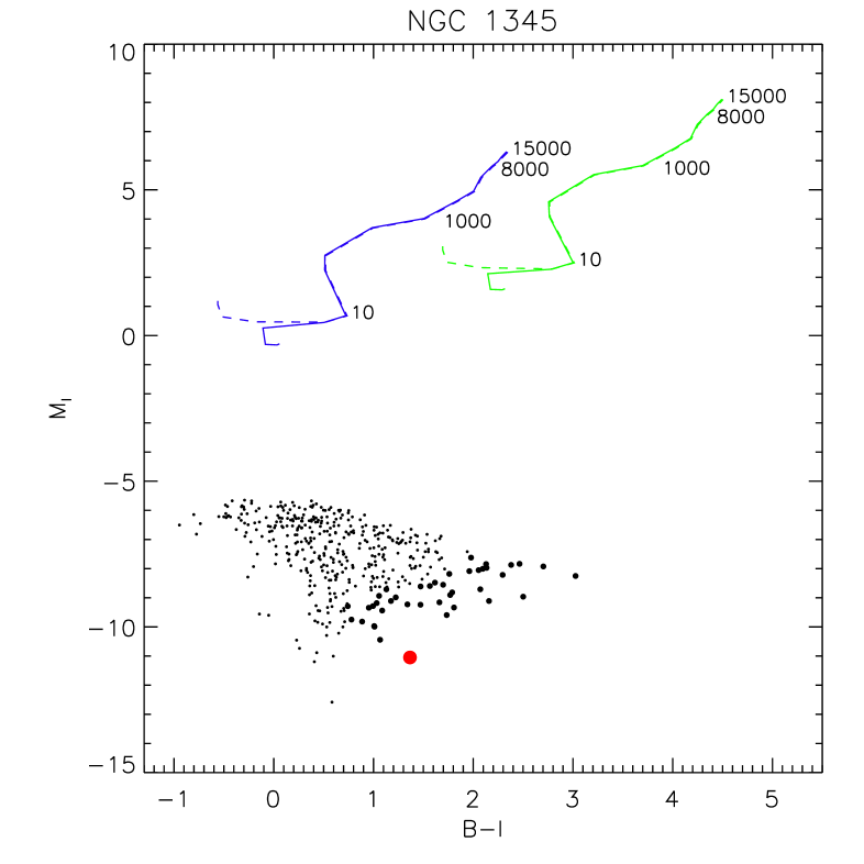
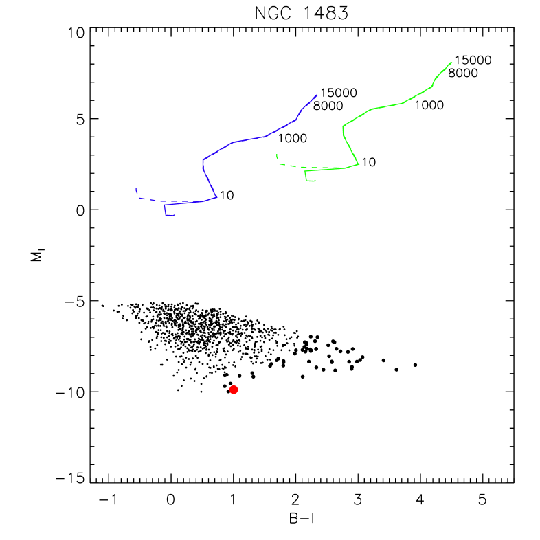
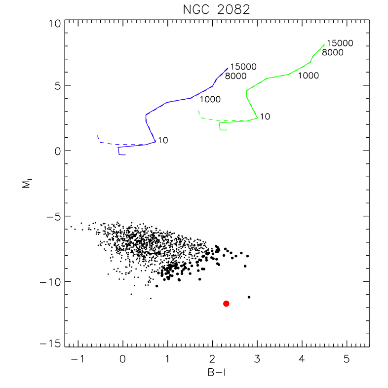
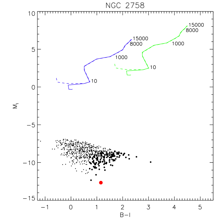
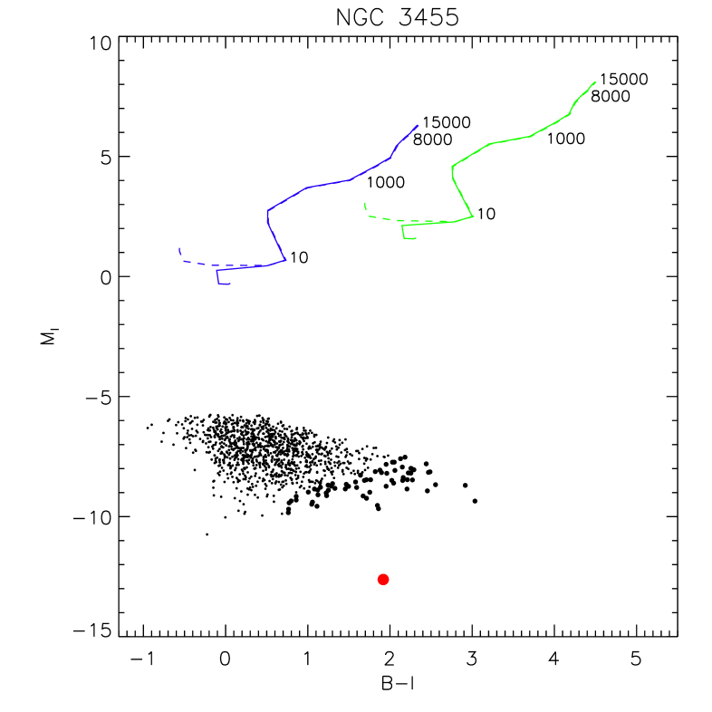
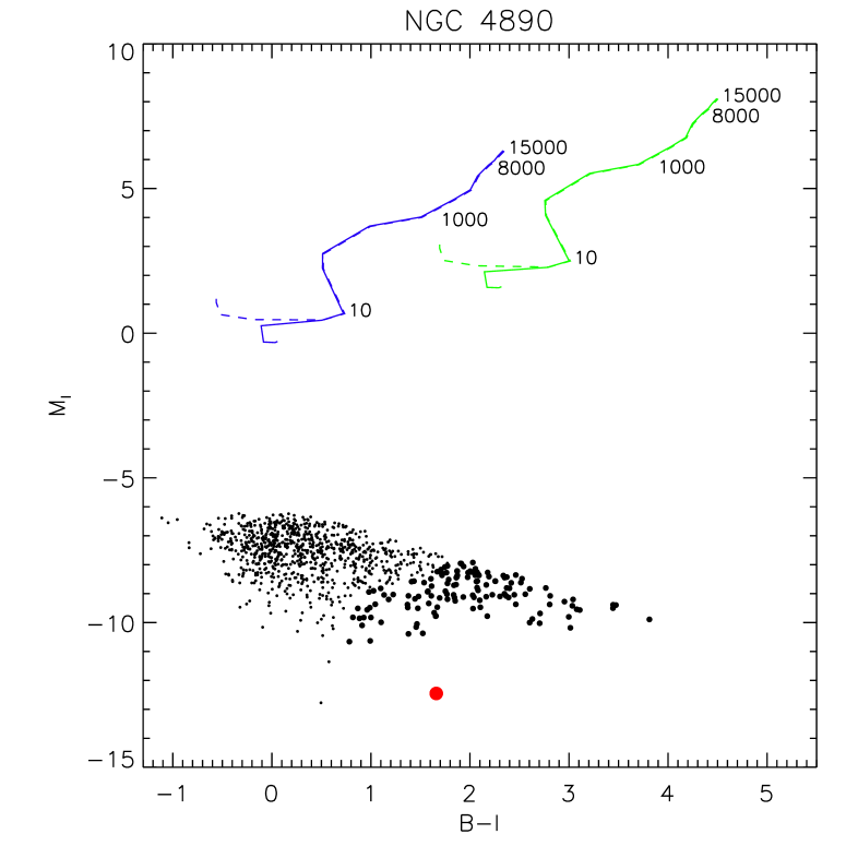
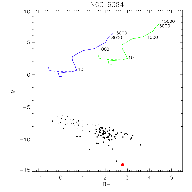
Figure 6: As in Fig. 5 but for the color-magnitude diagram ($B-I$ vs. $M_{I}$) for each galaxy compared to the Bruzual & Charlot (2003) models with a Salpeter IMF. Here the tracks for the models are shown for a total model mass of 1 $\mathrm{M_{\sun}}$. Therefore the difference in $M_{I}$ magnitude between an observed source and the model with a corresponding $B-I$ color gives the total mass of the observed star cluster. In addition, we show, as dashed lines, tracks without emission lines. The upper envelope of the data points is a selection effect given by the magnitude threshold of the survey.

A better diagnostic is provided by a color ($B-I$) vs. magnitude ($M_{I}$) diagram (see fig. 6 where the $M_{I}$ magnitude of the model tracks is computed for a reference 1 $\mathrm{M_{\sun}}$ mass). We can estimate the total mass of each observed source based on the difference in $M_{I}$ magnitude compared to the model with the same $B-I$ color. The $B-I$ color also highlights that up to $50\%$ of the total detected sources are younger than 8 Myr (see Table 3) under the assumption of no dust (again, see section 5.1 for a discussion of the possible impact of dust extinction). In all galaxies, the observed sources are clearly not distributed as an evolutionary sequence at constant mass. Instead the older the stellar population, the greater is its luminosity (and hence mass, because the mass-to-light ratio increases with age). This is consistent with the infant-mortality scenario for star clusters (Fall et al., 2005), in which only a small fraction of star clusters (usually the most massive) survives over time.

Every galaxy in our sample has a number of young star clusters, with ages $\lesssim$ 8 ${\rm Myr}$ and masses of the order of $10^{3}$ ${\mathrm{M}_{\sun}}$. These can be used to reconstruct the recent star formation history of the parent galaxies. Taken at face value, our results indicate an average recent star formation rate, in such clusters, of $0.1-0.01$ $\mathrm{M_{\sun}/yr}$. Linking this SFR to the actual SFR is however challenging, both because we need to extrapolate our results to young clusters below the detection threshold and because the photometric uncertainties might introduce a Malquist bias difficult to quantify. Conservatively we can consider our results a lower limit to the overall galaxy SFR.

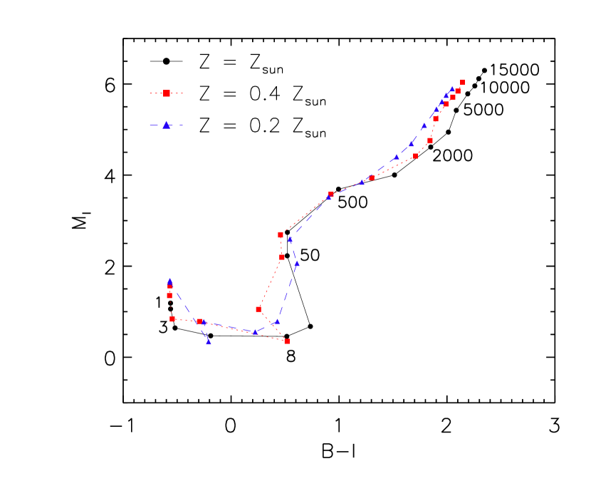
Figure 7: Color-magnitude diagram ($B-I$ vs. $M_{I}$) tracks for Bruzual & Charlot (2003) models for different metallicities (solid black line and dots: ${\mathrm{Z}_{\sun}}$; red dotted line and squares: 0.4 ${\mathrm{Z}_{\sun}}$; blue dashed line and triangles: 0.2 ${\mathrm{Z}_{\sun}}$). The plot highlights that there is relatively little metallicity dependence. Ages in Myr are superimposed on the tracks.

In this paper we focus on the properties of the oldest (age $\geqslant$ 250 Myr) and most massive ($M\geqslant 10^{5}$ ${\mathrm{M}_{\sun}}$) stellar clusters; for reasons discussed further below, we identify these as young candidate globular clusters. Our choice in age is an operational choice to avoid (i) the youngest systems, where stellar evolution of the most massive stars can influence the dynamical evolution of the system by their high mass-loss rates and (ii) a knee in the luminosity color relation (see Fig. 6) that would lead to a degeneracy in the mass estimate for the sources. Once a metallicity for the stellar population is assumed, the age and mass selection translates into a single color and luminosity selection respectively. If we assume a low metallicity ($Z=0.02$ ${\mathrm{Z}_{\sun}}$), the nuclear star cluster age turns out to be longer than the Hubble time, suggesting that these galaxies are more metal enriched (at least in their central regions studied here). For a metallicity range from 0.2 to 1 ${\mathrm{Z}_{\sun}}$ the total number of sources selected as globular cluster candidates varies at the 15% level at most. In fact, the tracks at different metallicities are close to each other for objects older than 250 Myr (see Fig. 7).

Therefore, in the following we adopt solar metallicity for the clusters. The age selection $\geqslant 250$ Myr then translates into a color selection $(B-I)\geqslant 0.73$ mag, assuming no dust. The same color cut corresponds instead to a younger age selection (age $\gtrsim 100$ Myr) if dust is present (see section 5.1). Our mass selection ($M\geqslant 10^{5}$ ${\mathrm{M}_{\sun}}$) translates into a cut-off luminosity that depends on the color of the source: all the sources whose magnitude is brighter than the corresponding 1 $M_{\odot}$ BC03 track, shifted by 12.5 mag, are accepted. Our selection has been carried out with the assumption of a Salpeter IMF. The luminosity cutoff we use refers instead to a mass $M\geqslant 5.6\cdot 10^{4}$ ${\mathrm{M}_{\sun}}$ if we were to assume a Chabrier IMF. We identify these older clusters as young candidate globular clusters since we calculate (Trenti et al., 2007) that they have more than a 50% probability of surviving tidal dissolution over a Hubble time, assuming they orbit within a point-like potential well. In addition, the age selection we apply (age $>$ 100-250 Myr) is sufficiently long to rule out early dissolution by supernova feedback.

For each galaxy, the candidate globular cluster luminosity function (GCLF), i.e. the number of candidate globular clusters per unit of magnitude, is plotted in Fig. 8. For all the galaxies, the GCLF (completeness corrected) is reasonably fitted by a Gaussian distribution, whose FWHM and peak magnitude are reported in Table 5. The residuals from the fit are somewhat asymmetric with an excess of faint sources. This might reflect an intrinsic skewness of the GCLF, which is however difficult to assert based on our data. Alternatively, it might be due to the presence of a small fraction of stellar contaminants with a luminosity distribution peaked at the faint end of the candidate globular cluster luminosity distribution (see Section 5.2). Note that dust extinction does not introduce skewness in the GCLF, but only changes its peak value unless the amount of dust present correlates with the luminosity of the star clusters.

5 Systematic Uncertainties

The results in section 4 are derived under the assumption of no dust extinction present outside the Milky Way and of absence of contamination in our sample. Here we discuss these two issues.

5.1 Dust Extinction

All the galaxies in our sample have NICMOS F160W coverage in the central region, which we use to quantify the impact of dust extinction. The F160W band is ideal, since in combination with the other bands we consider, it significantly increases the wavelength baseline. However the more limited field of view of NICMOS does not allow us to apply this diagnostic to the complete sample.

For the subsample of star cluster sources within the NICMOS field of view we perform a minimum chi-square fit on the data in four photometric bands comparing them to single stellar population models with a variable amount of dust extinction. We have three free parameters: the total stellar mass of the source, its age and its dust content. The fit is performed assuming different extinction laws within SYNPHOT: Galactic, LMC and SMC. As expected, the best fitting models with dust tend to be younger than their counterparts with no extinction. The estimation of the total mass of the sources is instead not strongly modified by allowing this additional degree of freedom.

We summarize the results of these fits in Table 4, where we give the number of sources older than $100$ Myr and more massive than $10^{5}\mathrm{M_{\sun}}$, for different assumed extinction laws. These results are compared, in the same table, to those obtained assuming an age $\geqslant 250$ Myr and no dust, and it may be seen that the estimates are within a factor two of each other. The difference between an age of $100$ and $250$ Myr is not very significant within the context of infant star-cluster mortality: in fact, most mortality happens within the first $50$ to $100$ Myr and is connected to mass loss induced by the rapid stellar evolution of the most massive stars in the cluster (Parmentier, 2009).

To take into account the effects of dust on the general sample, where NICMOS coverage is absent, we introduce a galaxy-dependent statistical correction $f_{ext-bias}$ to the total number of sources we define “massive” and “old” star clusters. $f_{ext-bias}$ (reported in the last column of Table 5) is computed within the NICMOS field of view as the fractional difference between the average number of sources identified in the presence of dust vs. the number identified under the no-dust assumption. This correction for dust extinction is then applied when we use the number of old star clusters obtained from the no-dust scenario to derive their specific frequencies (see Section 6).

The correction $f_{ext-bias}$ is conservative. In fact, based on the likelihood ratio test, the statistical significance of dust-extinction is above the 90% confidence level only for about one third of the sources with NICMOS coverage. This means that for some of the sources the apparent detection of non-zero extinction might simply be a consequence of allowing an additional degree of freedom in the fit. Finally, the NICMOS field of view is located at the center of the galaxy, where the amount of extinction is maximal (e.g. see Holwerda et al. 2005). The star clusters outside the NICMOS field of view are thus expected to be less influenced by dust.

5.2 Sample Contamination

A second systematic source of uncertainty that needs to be evaluated is the presence of stellar contaminants in our sample. These could either be stars in the Milky Way too faint to be identified by the presence of diffraction spikes or super-giants in the host galaxy.

To quantify the impact of Milky Way interlopers, in each galaxy of our sample we selected a region of the ACS field as far away from the galaxy as possible, with an area comparable to that used to search for star clusters. On these external regions we selected sources using the B and I bands according to the selection criteria we apply to old star clusters. The surface density of sources identified in the outskirts of the field of view is an upper limit to the number of Galactic contaminants. For all the 11 galaxies we obtained surface densities from 1 to 5 % (average 2.5%) of that of old star clusters selected in our main search region, therefore we can rest assured that Galactic stars are a negligible source of contamination compared to the larger uncertainties related to the treatment of dust extinction.

To quantify the impact of bright stars in the host galaxy, we consider the models of Marigo et al. (2008), that provide luminosities for giant-branch stars. Even for very low metallicities ($Z=10^{-4}Z_{\sun}$), the maximum luminosity of giant stars is $M_{V}>-7$; for higher metallicities the peak luminosity decreases (Marigo et al., 2008). From our Fig. 8 it is immediate to see that at most a few percent of the sources we select as star clusters are fainter than $M_{V}=-7$. Brighter contaminants are possible if they are young, extremely massive stars. These rare hypergiants can reach $M_{V}\sim~{}-10$ and exhibit a wide range of colors (e.g. see de Jager 1998 for a review). However, they are very short lived (a few million years) and thus not likely to be found outside the HII regions where they were born. Ideally we would need images in a narrow filter centered around the H-$\alpha$ emission line to identify these sources. As this is not available for our galaxies, we estimate their impact on the sample based on the measured star formation rate. Assuming a Salpeter IMF, we expect from a few to $\sim 10$ stars with mass $M>60~{}\mathrm{M_{\sun}}$ (bright enough to reach $M_{V}<-7$, e.g. see Stothers & Chin 1999 ) to enter in our selection for each galaxy. Combining these two sources of stellar contaminants, that is Galactic and extragalactic stars, we assume a fraction 10% of sample-contamination (indicated as $f_{cont}$ in Table 5). While this might carry some uncertainty, its impact is certainly secondary compared to the one induced by extinction, except for ESO 498G5 and NGC 6384.

6 Specific Frequency

For each galaxy, we calculate the specific frequency of the candidate globular clusters in our field of view, i.e. the older, more massive cluster population normalized to the host galaxy luminosity (see Table 6). This is defined as follows:

$${S_{N}}_{gal}=N_{tot}\cdot 10^{0.4({M_{V_{JC}}}_{gal}+15)},$$ (4)

where ${M_{V_{JC}}}_{gal}$ is the absolute magnitude of the galaxy within the search area in the Johnson-Cousins V-band and $N_{tot}$ (reported in Table 5) is the total number of candidate GCs, obtained by integrating the completeness-corrected GCLF and applying a correction $f_{cont}=0.1$ for the estimated fraction of stellar contaminants and a galaxy-dependent correction $f_{ext-bias}$ to take into account dust extinction (see section 5.2). The luminosity of the host galaxy within the star-cluster-search area in the HST-F606W filter is calculated through aperture photometry. The background level is estimated using the WF chips of WFPC2, which cover a larger region of the sky compared to the star-cluster-search area, limited within the PC chip. The F606W magnitude ($V$) is then converted to the Johnson-Cousins $M_{V_{JC}}$ absolute magnitude using:

$$M_{V_{JC}}=V+0.287\cdot(V-I)+dm,$$ (5)

where $dm$ is the distance modulus, listed in Table 1 and the color $V-I$ is from Carollo et al. (2007), except for NGC 1345 (for this galaxy the color is calculated from the photometry of the galaxy search area in both images). The coefficient 0.287 is obtained by fitting with a linear law the relation between $M_{V_{JC}}$ and $V-I$ for the Bruzual & Charlot (2003) models of old star clusters (magnitudes computed with the IRAF task CALCBAND). Eq. 5 agrees very well with the calibration given by Holtzman et al. (1995) in his Table 10 (maximum difference of 0.05 mag. in the range $-1<V-I<2$), but has two advantages. First it is calibrated exactly on the color range we are interested in (see the caveats in Holtzman et al. 1995 on the limited range of validity for his conversion) and second our formula is calibrated on the class of sources in which we are interested (star clusters, i.e. adopting an IMF) rather than individual stars as in Holtzman et al. (1995). In computing the specific frequencies we have excluded NGC 1483 (the closest galaxy in our sample) because its bulge is very extended spatially and it gives the dominant contribution to the light within the star-clusters search area.

The resulting values of ${S_{N}}_{gal}$ are listed in Table 6, where uncertainties on $S_{N}$ take into account the errors on the candidate GC count ($N_{tot}$), including those derived from dust extinction (see section 5.1), but not those in the distance modulus as they are negligible compared to the other errors.

The definition of specific frequency adopted here is a generalization of the standard Harris & van den Bergh (1981) definition, which is based on the total luminosity of the galaxy and on the total number of GCs. We note though that we do not expect a large difference in the two definitions, because the PC camera of WFPC2 contains a large fraction of the total light of the galaxies. Indeed, the absolute visual magnitude ${M_{V_{JC}}}_{gal}$ we measure in our sample differs by less than about 1 magnitude compared to the total $M_{V_{JC}}$ luminosity of the galaxy (estimated from the absolute blue magnitude reported in Table 1, assuming $B-V=0.5$).

We also compute the specific frequency relative to the bulge luminosity (${S_{N}}_{bul}$), defined as:

$${S_{N}}_{bul}=N_{tot}\cdot 10^{0.4({M_{V_{JC}}}_{bul}+15)},$$ (6)

where again ${M_{V_{JC}}}_{bul}$ is expressed in the Johnson-Cousins system, obtained as above from the bulge $V$-magnitude published by Carollo et al. (2007). The resulting frequencies of candidate globular clusters per bulge light are also shown in Table 6.

These frequencies for our sample of galaxies can be compared with published values for nucleated dwarf galaxies (Miller et al., 1998), as well as for early and late type galaxies with classical bulges (see Brodie & Strader 2006). The ${S_{N}}_{gal}$ we measure in our late type galaxies is qualitatively consistent with that of other spiral galaxies, but there is a moderate tendency toward higher $S_{N}$. This finding seems to be at odd with predictions from semi-analytics models of globular clusters formation which link the specific frequency with the overall star formation rate of the galaxy (Beasley et al., 2002): based on their scenario we would have expected a lower $S_{N}$ for our sample compared to that of spiral galaxies with classical bulges. In fact, we expect a lower star formation rate in pseudo-bulges if they form from the inner disk. However the Beasley et al. (2002) study was aimed at reproducing the properties of GCs in elliptical galaxies, therefore the comparison is only indirect, based on the assumption that the bulge formation process is similar to that of small ellipticals. In addition, it did not include evolution of the GCs system of the simulated galaxies, but rather its properties were fixed and fine tuned to match the observed data at the time of birth.

Another possibility to reconcile with these theoretical expectations is that of disruption of our candidate globular clusters as they age. Most of the ‘old’ star clusters in our sample appear in fact to be relatively young compared to Galactic globular clusters (ages from a few hundred Myr to one Gyr), so this suggests that tidal interactions with the parent galaxies will reduce the number of star clusters as they age. For example, Gnedin & Ostriker (1997) estimate that for the Milky Way, the Galactic globular cluster system has an half life of the order of the Hubble time. This is consistent with detailed N-body simulations of the dynamics of star clusters in the presence of a tidal field (e.g. see Trenti et al. 2007 and references therein). Under a scenario of significant adult mortality for star clusters, the specific frequency for our sample will become lower than that of spirals with a classical bulge, as expected on the basis of theoretical modeling of star formation (SF): in the case of pseudo-bulges, with a likely extended but low-efficiency star formation history, fewer globular clusters are formed than in an equivalent burst of SF, such as that considered to create classical bulges (Kormendy & Kennicutt, 2004).

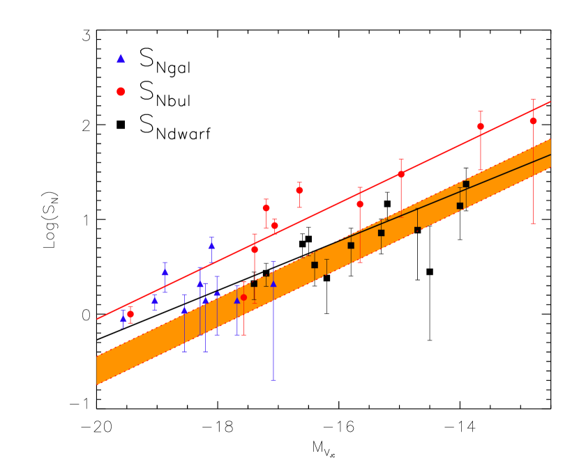
Figure 9: Candidate globular cluster specific frequencies in our sample (normalized to the galaxy luminosity: blue triangles; normalized to the bulge luminosity: red circles). For comparison the globular cluster specific frequencies for the sample of dwarf ellipticals of Miller et al. (1998) are plotted as black squares. The solid red (specific frequency normalized to bulge luminosity) and black (specific frequency for dwarf ellipticals) lines represent a best fitting linear relation in the ($Log(S_{N});M_{V_{JC}}$) space. The orange region delimited by the red dotted lines is a passive evolution of the solid red line, assuming that the bulge population ages from 1 to 10 Gyr (corresponding to a dimming of $\approx 2.2$ mag in $M_{V}$) and a reduction in the number of star clusters due to tidal dissolution (50%) and stripping due to galaxy harassment (50% to 75%).

Mean specific frequencies for nucleated dwarf galaxies ($\langle{S_{N}}_{dwarf}\rangle=7.5$) — whose GCs are similar to candidate GCs in our sample — lie instead between our $\langle{S_{N}}_{gal}\rangle=2.0$ and $\langle{S_{N}}_{bul}\rangle=30$. In addition, the trend of frequencies of candidate globular clusters per bulge light versus luminosity is very similar to that of dwarf galaxies (see Fig. 9). This is suggestive of a stripping scenario in which dwarf galaxies originate from the bulges of late-type spirals. One possibility is that galaxy-galaxy fly-by encounters (galaxy harassment: Moore et al. 1996) may strip away stars in the disk, leaving preferentially behind bulge members and the central star clusters, both more protected because they sit deeper in the potential well of the system. In fact, passive evolution of the bulges (aging them from 1 to 10 Gyr, to model dwarf galaxies that have older stellar populations than pseudo-bulges) and accounting for tidal dissolution and stripping of star clusters (50 % tidal dissolution and 50% to 75% stripping) shift the candidate GC specific frequency vs. luminosity relation to match that valid for dwarf ellipticals (see Fig. 9).

7 Nuclear Star Clusters

A detailed study of the photometric properties of nuclear star clusters has been presented in Carollo et al. (1997, 1998, 2002), here we briefly discuss their inferred ages and dust content. A summary of the photometry for the central sources is reported in Table 7, while the resulting mass, age and dust content from our maximum likelihood fit are in Table 8. The nuclear star clusters in the sample are typically the brightest clusters of their host galaxies, with an inferred mass up to $\sim 10^{7}$ $\mathrm{M_{\sun}}$. The mass of the central star cluster broadly correlates with the bulge luminosity (and therefore mass), as observed in a wide sample of galaxies, both photometrically (e.g. Wehner & Harris 2006; Côté et al. 2006; Rossa et al. 2006) and dynamically from spectroscopy (e.g. Geha et al. 2002; Walcher et al. 2006). The correlation is consistent with Fig. 1 in Wehner & Harris (2006). Like in the Wehner & Harris (2006) work, we identify a few clusters (NGC 406, NGC 1345 and NGC 2758) with a bright bulge ($\sim 10^{8.5}~{}\mathrm{L_{\sun}}$), but with a relatively small nuclear star cluster mass ($\sim 2\cdot 10^{6}~{}\mathrm{M_{\sun}}$).

From the nuclear star cluster colors we infer a typical age $\gtrsim 1$ Gyr in most of the sample, even after accounting for a variable dust extinction as described in section 5.1. Two galaxies (NGC 1483, NGC 2758) present a clear evidence that their nuclear star cluster is composed of a young stellar population (age $5-50$ Myr) associated with dust ($E(B-V)>0.2$). The nuclear star cluster of NGC 3259 has instead colors that are poorly fitted by both models with and without dust extinction: no reliable constrain on the stellar age can be obtained. The younger stellar ages observed in the nuclear clusters of NGC 1483 and NGC 2758 might be due to a recent burst of star formation at the center of these galaxies that has rejuvenated them. This is not surprising as rejuvenation is observed in a large number of nuclear star clusters (Rossa et al., 2006; Walcher et al., 2006) and suggests a in situ formation scenario for the clusters, as proposed by Milosavljević (2004) and inferred from observations of local spirals by Seth et al. (2006). However the relative old ages ($\gtrsim 1$ Gyr) of most of the sources are also consistent with a formation scenario driven by mergers of star clusters that reach the center of the galaxy by dynamical friction (Tremaine et al., 1975; Lotz et al., 2001; Andersen et al., 2008).

8 Discussion and Conclusion

In this paper we studied the properties of (relatively) old star clusters in a sample of 11 late-type spiral galaxies selected for the presence of a pseudo-bulge (Carollo et al., 1997). Star clusters were classified based on their color and luminosity through comparison of population synthesis models with HST photometry in three bands (ACS F435W, F814W and WFPC2 F606W). By means of artificial source detections we estimated a completeness of $\simeq 50\%$ down to $V=25.5$. The clusters in our sample present a wide range of ages and masses, from young blue clusters with ages of a few tens of Myrs to an older, red population (age $>100-250$ Myr). We focus on these older, red clusters and identify them as young globular cluster candidates.

All these galaxies have massive nuclear star clusters with masses in the $10^{6}-10^{7}~{}\mathrm{M_{\sun}}$ range. These sources are typically the brightest star clusters in their host galaxy. They have a relatively old stellar age ($\gtrsim$ 1 Gyr) except for two cases where a younger and dusty stellar population is inferred. Overall, the properties of our sample appear consistent with both proposed formation scenarios for nuclear star clusters, namely merging of stellar clusters driven to the galaxy center by dynamical friction (Lotz et al., 2001) or in situ formation (Milosavljević, 2004).

The presence of a young star clusters allows us to set a lower limit to the star formation rate in the galaxies, which turns out to be $0.1-0.01$ $\mathrm{M_{\sun}/yr}$. This continuous, low rate of star formation is consistent with the formation scenario for pseudo-bulges, postulated to arise out of secular processes in the disk (Kormendy & Kennicutt, 2004), compared to a violent burst of SF needed to form a classical bulge.

Based on the Kormendy & Kennicutt (2004) discussion of the formation of pseudo-bulges, we would expect them to have a deficit of massive star clusters compared to spirals with classical bulges, but this is not what we find. On the contrary, the specific frequencies (number of star clusters normalized to the galaxy luminosity — Harris & van den Bergh 1981) for the old population is consistent, within our uncertainties, to published data for other spirals. This appears to be a solid result, especially since we considered only central star clusters (the WFCP2 high resolution detector limits our area of search to the central $35\arcsec\times 35\arcsec$), normalizing the specific frequency to the galaxy luminosity within the field of view: in general star cluster systems are more spatially extended than their host galaxy (e.g. see Djorgovski & Meylan 1994; Jordán et al. 2009), thus our specific frequencies are probably lower limits to the global specific frequency.

When the specific frequency is computed with respect to the bulge luminosity we get even higher $S_{N}$. Interestingly the specific frequency vs. bulge magnitude ${S_{N}}_{bul}({M_{V_{JC}}}_{bul})$ trend is similar to the one observed in dwarf ellipticals. Pseudo-bulges have photometric and kinematic properties very similar to dwarf ellipticals, thus it is suggestive that some dwarf ellipticals might be the result of evolution of spiral galaxies with pseudo-bulges: the galaxy disk might in fact be stripped during galaxy-galaxy interactions (galaxy harassment — Moore et al. 1996). In this scenario star clusters are also stripped away, but still a sizable number might survive compared to the more spatially extended disk. At the same time the pseudo-bulge survives almost untouched by stripping, protected as it sits at the center of the galaxy potential well. While this scenario is overall appealing, detailed numerical simulations are needed for a proper validation. These will be presented in a follow-up paper.

Figure 8: Solid lines: Candidate Globular Cluster Luminosity Functions in the V-band, completeness-corrected, with the best-fitting Gaussian superposed. Dotted lines show the GCLF without completeness correction. No extinction or contamination correction has been applied. The black dot corresponds to the nuclear star cluster of each galaxy. The histograms ($\frac{dN(M_{V})}{dM_{V}}$) are normalized so that the total number of observed sources $N=\int_{M_{V}}\frac{dN(M_{V})}{dM_{V}}dM_{V}$.

Table 1: Basic parameters for the sample galaxies.

Name	$\alpha$(J2000)	$\delta$(J2000)	$B_{tot}$	D	dm	$M_{B_{tot}}$	Type	E(B-V)	$R_{search}$
	(h m s)	(deg ′ ″)	(mag)	(Mpc)	(mag)	(mag)		(mag)	(kpc)
ESO 498G5	09 24 41.10	-25 05 33.0	13.96	37.7	32.88	-18.92	SXS4P/SBbc	0.107	3.254
ESO 499G37	10 03 42.10	-27 01 39.0	13.15	17.7	31.24	-18.09	SXS7*/SBc	0.075	1.529
NGC 406	01 07 24.10	-69 52 35.0	13.10	19.8	31.48	-19.38	SAS5*/Sc	0.024	1.708
NGC 1345	03 29 31.70	-17 46 42.0	14.02	19.1	31.41	-17.39	SBS5P/SBa	0.038	1.654
NGC 1483	03 52 47.60	-47 28 39.0	13.00	15.1	30.90	-17.90	SBS4/Sb-Sc	0.007	1.308
NGC 2082	05 41 51.20	-64 18 04.0	12.62	17.1	31.17	-18.55	SBR3/SBb	0.058	1.481
NGC 2758	09 05 30.80	-19 02 38.0	13.46	31.3	32.48	-18.02	PSB.4P?/Sbc	0.126	2.707
NGC 3259	10 32 34.68	+65 02 26.8	12.97	24.8	31.97	-19.00	SXT4*/SBbc	0.015	2.140
NGC 3455	10 54 31.20	+17 17 02.8	12.87	19.8	31.48	-18.61	PSXT3/Sb	0.033	1.708
NGC 4980	13 09 10.20	-28 38 28.0	13.19	23.9	31.89	-18.70	SXT1P?/SBa	0.072	2.063
NGC 6384	17 32 24.42	+07 03 36.8	11.14	22.4	31.75	-20.61	SXR4/SBbc	0.123	1.934

Note. — Right Ascension ($\alpha$), declination ($\delta$) and total apparent blue magnitude ($B_{tot}$) are from RC3 catalog (de Vaucouleurs et al., 1991). Distance ($D$) and distance modulus ($dm$) are from the online NASA/IPAC Extragalactic Database (NED). The absolute magnitude $M_{B_{tot}}$ is obtained from $B_{tot}$ and $dm$. Morphological classifications are from the RC3 (left) and from the UGC (right) catalogs. The color excess E(B-V) is taken from Schlegel et al. (1998). The last column lists the radius of the common ACS/WFC-WFPC2/PC field of view.

Table 2: Details of the photometric calibration.

Filter	Zeropoint	Threshold	Reddening
	(mag)	(mag)	(mag)
F435W (ACS/WFC)	25.779	26.5	1.319
F606W (WFPC2/PC)	22.084	26	0.908
F814W (ACS/WFC)	25.501	26	0.586

Note. — Zeropoints used for calibrating the magnitudes, threshold magnitudes corresponding to a SNR $\sim 5$ and reddening coefficients expressed as $A_{HSTfilter}/A_{{V}_{JC}}$.

Table 3: Number of observed Star Clusters.

Name	All	Age $\leqslant$ 8 Myr	Age $\geqslant$ 250 Myr
ESO 498G5	477	225	62
ESO 499G37	434	230	53
NGC 406	1058	376	133
NGC 1345	490	194	41
NGC 1483	1208	551	59
NGC 2082	1401	576	96
NGC 2758	777	326	141
NGC 3259	805	409	70
NGC 3455	1317	623	67
NGC 4980	1070	591	133
NGC 6384	153	25	71

Note. — For each galaxy (first column) the total number of sources identified as star clusters is given in the second column, while the number of young (age $\leqslant$ 8 Myr) and old (age $\geqslant$ 250 Myr) star clusters is in the third and fourth column respectively.

Table 4: Star Cluster counts with extinction.

Name	$(N\geqslant 100~{}\mathrm{Myr})_{Gal-Ext}$	$(N\geqslant 100~{}\mathrm{Myr})_{LMC-Ext}$	$(N\geqslant 100~{}\mathrm{Myr})_{SMC-Ext}$	$(N\geqslant 250~{}\mathrm{Myr})_{NO-Dust}$
ESO 498G5	7	3	6	5
ESO 499G37	2	1	1	5
NGC 406	17	14	17	23
NGC 1345	10	8	12	18
NGC 1483	1	1	1	10
NGC 2082	8	3	7	18
NGC 2758	15	11	13	20
NGC 3259	7	5	6	14
NGC 3455	3	3	3	7
NGC 4980	7	5	8	19
NGC 6384	6	5	5	6

Note. — Number of star clusters more massive than $10^{5}~{}\mathrm{M_{\sun}}$ and with age $\geqslant 100$ Myr identified in the central region of the galaxies within the NICMOS F160W field of view. The number of sources has been obtained using a least chi-squared fit of the four band photometry (F435W, F606W, F814W & F160W) allowing for a variable amount of dust extinction with different extinction laws (Galactic: second column, LMC third column and SMC fourth column). The last column reports the number of sources within the same field of view that are older than $250$ Myr and more massive than $10^{5}~{}\mathrm{M_{\sun}}$ when the fit is forced to have no dust extinction.

Table 5: Candidate Globular Cluster Luminosity Function fitted as a Gaussian.

Name	$M_{V_{peak}}$	FWHM	$N_{fit}$	$f_{cont}$	$f_{ext-bias}$	$N_{tot}$
ESO 498G5	-9.32$\pm$0.09	1.46$\pm$0.14	67$\pm$10	0.1	$<$ 0.05	$57^{+10}_{-10}$
ESO 499G37	-7.69$\pm$0.10	1.46$\pm$0.15	53$\pm$9	0.1	0.70	$14^{+10}_{-13}$
NGC 406	-7.86$\pm$0.09	2.15$\pm$0.15	147$\pm$15	0.1	0.30	$92^{+20}_{-31}$
NGC 1345	-8.56$\pm$0.14	1.80$\pm$0.26	33$\pm$6	0.1	0.45	$16^{+7}_{-10}$
NGC 1483	-6.87$\pm$0.13	2.01$\pm$0.22	61$\pm$9	0.1	0.90	$5^{+4}_{-4}$
NGC 2082	-8.16$\pm$0.12	2.13$\pm$0.20	84$\pm$10	0.1	0.65	$26^{+13}_{-20}$
NGC 2758	-8.75$\pm$0.08	2.08$\pm$0.13	171$\pm$17	0.1	0.35	$100^{+24}_{-39}$
NGC 3259	-8.45$\pm$0.08	1.49$\pm$0.14	72$\pm$10	0.1	0.55	$29^{+13}_{-19}$
NGC 3455	-7.91$\pm$0.12	2.00$\pm$0.19	69$\pm$10	0.1	0.55	$27^{+12}_{-18}$
NGC 4980	-8.12$\pm$0.08	1.92$\pm$0.14	139$\pm$14	0.1	0.65	$43^{+20}_{-32}$
NGC 6384	-8.34$\pm$0.11	1.93$\pm$0.19	76$\pm$11	0.1	0.10	$61^{+11}_{-12}$

Note. — Completeness corrected GCLF gaussian fit for the galaxies in our sample (first column). Fitted peak $M_{V}$-magnitude and FWHM are in the second and third columns respectively. The fourth column gives the total number of candidate globular clusters as inferred from the fit ($N_{fit}$ ). The fifth column contains the estimated fraction of stellar contaminants in our sample (see section 5.2). The sixth column gives the fractional bias in the number of old star clusters induced by dust extinction of their host galaxy (see section 5.1). The last column reports our fiducial number $N_{tot}$ of candidate globular clusters obtained, defined as $N_{tot}=N_{fit}\cdot(1-f_{cont})\cdot(1-f_{ext-bias})$.

Table 6: Specific frequencies of candidate GCs.

Name	$R_{search}$	${M_{V_{JC}}}_{gal}$	${S_{N}}_{gal}$	${M_{V_{JC}}}_{bul}$	${S_{N}}_{bul}$
	(kpc)	(mag)		(mag)
ESO 498G5	3.254	-19.04	$1.4^{+0.2}_{-0.3}$	-17.06	$8.6^{+1.5}_{-1.6}$
ESO 499G37	1.529	-17.08	$2.1^{+1.5}_{-1.9}$	-12.79	$110^{+75}_{-101}$
NGC 406	1.708	-18.01	$5.3^{+1.2}_{-1.8}$	-16.65	$20^{+4}_{-7}$
NGC 1345	1.654	-17.68	$1.4^{+0.6}_{-0.8}$	-17.57	$1.5^{+0.7}_{-0.9}$
NGC 2082	1.481	-18.20	$1.4^{+0.7}_{-1.0}$	-15.65	$14^{+7}_{-11}$
NGC 2758	2.707	-18.87	$2.8^{+0.7}_{-1.1}$	-17.20	$13^{+3}_{-5}$
NGC 3259	2.140	-18.55	$1.1^{+0.5}_{-0.7}$	-14.97	$30^{+13}_{-20}$
NGC 3455	1.708	-18.01	$1.7^{+0.8}_{-1.1}$	-13.66	$96^{+43}_{-63}$
NGC 4980	2.063	-18.29	$2.1^{+1.0}_{-1.5}$	-17.39	$5.0^{+2.2}_{-3.5}$
NGC 6384	1.934	-19.56	$0.9^{+0.2}_{-0.2}$	-19.44	$1.0^{+0.2}_{-0.2}$

Note. — Candidate globular cluster specific frequencies with respect to the galaxy luminosity (fourth column) and to the bulge luminosity (sixth column). The relevant luminosities used here are given in the third and fifth columns and are expressed in the Johnson-Cousins system. The galaxy luminosity has been obtained by considering the light within a circular region of radius $R_{search}$ (second column), corresponding to the search area for the star clusters. The bulge luminosity is from Carollo et al. (2007).

Table 7: Photometry of Nuclear Star Clusters.

Name	$\alpha$(J2000)	$\delta$(J2000)	$B$	$V$	$I$	$H$	$R_{B}$
	(h m s)	(deg ′ ″)	(mag)	(mag)	(mag)	(mag)	(arcsec)
ESO 498G5	09 24 40.68	-25 05 31.7	20.93$\pm$0.04	19.72$\pm$0.02	18.93$\pm$0.17	17.23$\pm$0.33	0.04$\pm$0.02
ESO 499G37	10 03 41.69	-27 01 38.1	20.2$\pm$0.1	19.32$\pm$0.05	18.8$\pm$0.25	18.35$\pm$0.35	0.25$\pm$0.05
NGC 406	01 07 24.48	-69 52 30.2	22.29$\pm$0.06	21.22$\pm$0.04	20.47$\pm$0.14	19.15$\pm$0.28	0.04$\pm$0.02
NGC 1345	03 29 31.66	-17 46 42.6	21.7$\pm$0.1	20.91$\pm$0.07	20.36$\pm$0.19	18.88$\pm$0.31	0.05$\pm$0.02
NGC 1483	03 52 47.65	-47 28 37.3	22.02$\pm$0.04	21.54$\pm$0.06	21.02$\pm$0.07	19.76$\pm$0.19	0.04$\pm$0.02
NGC 2082	05 41 50.92	-64 18 02.6	21.79$\pm$0.07	20.39$\pm$0.02	19.48$\pm$0.18	17.76$\pm$0.23	0.05$\pm$0.02
NGC 2758	09 05 31.17	-19 02 33.1	20.97$\pm$0.06	20.29$\pm$0.02	19.82$\pm$0.15	18.62$\pm$0.26	0.08$\pm$0.05
NGC 3259	10 32 34.67	+65 02 25.9	20.54$\pm$0.08	19.06$\pm$0.05	18.96$\pm$0.24	17.05$\pm$0.33	0.04$\pm$0.02
NGC 3455	10 54 31.12	+17 17 04.1	20.78$\pm$0.05	19.16$\pm$0.01	18.86$\pm$0.13	17.35$\pm$0.30	0.05$\pm$0.02
NGC 4980	13 09 10.18	-28 38 33.6	21.1$\pm$0.03	20.07$\pm$0.01	19.44$\pm$0.08	18.23$\pm$0.11	0.05$\pm$0.02
NGC 6384	17 32 24.27	+07 03 36.1	20.6$\pm$0.08	18.97$\pm$0.07	17.87$\pm$0.13	15.98$\pm$0.27	0.06$\pm$0.03

Note. — Summary of the photometric properties of nuclear star clusters for our sample of galaxies, listed in the first column. The second and third columns report the coordinates of the central star cluster, followed by apparent magnitudes ($B,~{}V,~{}I,~{}H$). The last column is an estimate of the half-light radius in the $B$ band, after deconvolution with the PSF.

Table 8: Properties of Nuclear Star Clusters.

Name	Mass	Age	$E(B-V)$
ESO 498G5	$5-12\cdot 10^{7}\mathrm{M_{\sun}}$	$5-13$ Gyr	0.06-0.2
ESO 499G37	$1.7-3.9\cdot 10^{6}\mathrm{M_{\sun}}$	$1-3$ Gyr	0-0.15
NGC 406	$1.8-3.9\cdot 10^{6}\mathrm{M_{\sun}}$	$2-5$ Gyr	0-0.2
NGC 1345	$1.1-1.7\cdot 10^{6}\mathrm{M_{\sun}}$	$1-2$ Gyr	0-0.25
NGC 1483	$0.2-1\cdot 10^{6}\mathrm{M_{\sun}}$	$8-50$ Myr	0.2-0.25
NGC 2082	$8.6-15\cdot 10^{7}\mathrm{M_{\sun}}$	5-12 Gyr	0.1-0.17
NGC 2758	$6-31\cdot 10^{5}\mathrm{M_{\sun}}$	5-50 Myr	0.5-0.7
NGC 3259	$2.5-21\cdot 10^{6}\mathrm{M_{\sun}}$	5-3000 Myr	0-1.17
NGC 3455	$1.1-2.8\cdot 10^{7}\mathrm{M_{\sun}}$	2-10 Gyr	0-0.24
NGC 4980	$8.1-26\cdot 10^{6}\mathrm{M_{\sun}}$	3-13 Gyr	0-0.03
NGC 6384	$8-20\cdot 10^{7}\mathrm{M_{\sun}}$	$2-13$ Gyr	0.2-0.8

Note. — Properties of the nuclear star clusters derived from the fit of photometric properties (see Tab. 7) using single-stellar population models. The range in Mass (second column), Age (third column) and Extinction (fourth column) is based on the range of acceptable $1~{}\sigma$ fits.

References

- Andersen et al. (2008) Andersen, D. R. et al. 2008, ApJ, 688, 990
- Andredakis et al. (1995) Andreadakis, Y. C., Peletier, R. F., Balcells, M. 1995, MNRAS, 275, 874
- Beasley et al. (2002) Beasley, M. A., Baugh C. M., Forbes, D. A., Sharples, R. M. & Frenk, C. S. 2002, MNRAS, 333, 383
- Bertin & Arnouts (1996) Bertin, E. & Arnouts, S. 1996, A&A117, 393
- Böker et al. (2004) Böker, T. and Sarzi, M. and McLaughlin, D. E. and van der Marel, R. P. and Rix, H.-W. and Ho, L. C. and Shields, J. C. 2004, AJ, 127, 105
- Brodie & Strader (2006) Brodie, J. P.& Strader, J. 2006, ARA&A, 44, 193
- Bruzual & Charlot (2003) Bruzual, G. & Charlot, S. 2003, MNRAS, 344, 1000
- Carollo et al. (1997) Carollo, C. M., Stiavelli, M., de Zeeuw, P. T. & Mack, J. 1997, AJ, 114, 2366
- Carollo et al. (1998) Carollo, C. M., Stiavelli, M. & Mack, J. 1998, AJ, 116, 68
- Carollo & Stiavelli (1998) Carollo, C. M. & Stiavelli, M. 1998, AJ, 115, 2306
- Carollo et al. (2002) Carollo, C. M., Stiavelli, M., Seigar, M., de Zeeuw, P. T. & Dejonghe, H. 2002, AJ, 123, 159
- Carollo et al. (2007) Carollo, C. M., Scarlata, C., Stiavelli, M., Wyse, R. F. G. & Mayer, L. 2007, ApJ, 658, 960
- Chabrier (2003) Chabrier, G. 2003, PASP, 115, 763
- Conselice, Gallagher & Wyse (2003) Conselice, C., Gallagher, J.S. & Wyse, R.F.G. 2003, AJ, 125, 66
- Côté et al. (2006) Côté, P. et al. 2006, ApJS, 165, 57
- de Vaucouleurs et al. (1991) de Vaucouleurs, G., de Vaucouleurs, A., Corwin, H., Buta, R. J., Paturel, G. & Fouque, P. 1991, Third Reference Catalogue of Bright Galaxies, New York: Springer-Verlag
- de Jager (1998) de Jager, C. 1998, A&A Rev., 8, 145
- Djorgovski & Meylan (1994) Djorgovski, S. G. & Meylan, G. 1994, AJ, 108, 1292
- Fall et al. (2005) Fall, S. M., Chandar, R. & Whitmore, B. C. 2005, ApJ, 631, 133
- Geha et al. (2002) Geha, M., Guhathakurta, P. & van der Marel, R. P. 2002, AJ, 124, 3073
- Gnedin & Ostriker (1997) Gnedin, O. Y. & Ostriker, J. P. 1997, ApJ, 474, 223
- Harris & van den Bergh (1981) Harris, W. E. & van den Bergh, S. 1981, AJ, 86, 1627
- Holtzman et al. (1995) Holtzman, J. A., Burrows, C. J., Casertano, S., Hester, J. J., Trauger, J. T., Watson, A. M. & Worthey, G. 1995, PASP, 107, 1065
- Holwerda et al. (2005) Holwerda, B. W., Gonzalez, R. A.; Allen, R. J.; van der Kruit, P. C. 2005, A&A, 129, 1396
- Jordán et al. (2009) Jordán, A. et al. 2009, ApJS, 180, 54
- Kormendy (1993) Kormendy, J. 1993 in IAU Symp. 153, Galactic Bulges, ed. H. Dejonghe & H. Habing (Dordrecht: Kluwer), 209
- Kormendy & Kennicutt (2004) Kormendy, J. & Kennicutt R. C. 2004, ARA&A, 42, 603
- Krist & Hook (2001) Krist, J. & Hook, R. 2001, “The TinyTim User’s Guide”, Version 6.0 (Baltimore: STScI)
- Lotz et al. (2001) Lotz, J. M. and Telford, R. and Ferguson, H. C. and Miller, B. W. and Stiavelli, M. and Mack, J. 2001, ApJ, 552, 572
- Marigo et al. (2008) Marigo, P. , Girardi, L., Bressan, A., Groenewegen, M. A. T., Silva, L., Granato, G. L. 2008, A&A, 482, 883
- Miller et al. (1997) Miller, B. W., Whitmore, B. C., Schweizer, F. & Fall, S. M. 1997, AJ, 114, 6
- Miller et al. (1998) Miller, B. W., Lotz, J. M., Ferguson, H. C., Stiavelli, M. & Whitmore, B. C. 1998 ApJ, 508, 133
- Milosavljević (2004) Milosavljević, M. 2004, ApJ, 605, 13
- Mobasher & Roye (2004) Mobasher, B. & Roye, E. 2004, “NICMOS Data Handbook”, Version 6.0 (Baltimore: STScI)
- Moore et al. (1996) Moore, B., Katz, N., Lake, G., Dressler, A. & Oemler, A. 1996, Nature, 379, 613
- Oesch et al. (2007) Oesch, P. A., Stiavelli, M., Carollo, C. M., Bergeron, L. E., Koekemoer, A. M., Lucas, R. A., Pavlovsky, C. M., Trenti, M., Lilly, S. J., Beckwith, S. V. W., Dahlen, T., Ferguson, H. C., Gardner, J. P., Lacey, C., Mobasher, B., Panagia, N. & Rix, H. W. 2007, ApJ, 671, 1212
- Parmentier (2009) Parmentier, G. 2009, MNRAS, 377, 352, arxiv:0901.3140
- Pavlovsky et al. (2006) Pavlovsky, C. M., et al. 2006, “ACS Data Handbook”, Version 5.0 (Baltimore: STScI)
- Rossa et al. (2006) Rossa, J. et al. 2006, AJ, 103, 1074
- Schlegel et al. (1998) Schlegel, D. J., Finkbeiner, D. P. & Davis, M. 1998, ApJ, 500, 525
- Salpeter (1955) Salpeter, E. E. 1955, ApJ, 121, 161
- Seigar et al. (2002) Seigar, M., Carollo, C. M., Stiavelli, M., de Zeeuw, P. T. & Dejonghe, H. 2002, AJ, 123, 184
- Seth et al. (2006) Seth, A. C. and Dalcanton, J. J. and Hodge, P. W. and Debattista, V. P. 2006, AJ, 132, 2539
- Stiavelli et al. (2001) Stiavelli, M., Miller, B. W., Ferguson, H., Mack, J., Whitmore, B. C., Lotz, J. M. 2001, ApJ, 121, 1385.
- Stothers & Chin (1999) Stothers, R. B. and Chin, C.-W. 1999, ApJ, 522, 960
- Tremaine et al. (1975) Tremaine, S. D. and Ostriker, J. P. and Spitzer, Jr., L. 1975, ApJ, 196, 407
- Trenti et al. (2007) Trenti, M., Heggie, D. C. & Hut, P. 2007, 374, 344
- Walcher et al. (2005) Walcher, C. J. et al. 2005, ApJ, 618, 237
- Walcher et al. (2006) Walcher, C. J. et al. 2006, ApJ, 649, 692
- Wehner & Harris (2006) Wehner, E. H. & Harris, W. E. 2006, ApJ, 644, 17