Interaction Quenches of Fermi Gases

Abstract

It is shown that the jump in the momentum distribution of Fermi gases evolves smoothly for small and intermediate times once an interaction between the fermions is suddenly switched on. The jump does not vanish abruptly. The loci in momentum space where the jumps occur are those of the noninteracting Fermi sea. No relaxation of the Fermi surface geometry takes place.

Recently, the interest in nonequilibrium quantum physics has risen significantly. This is due to experimental and theoretical progress in treating quantum systems with time dependent parameters. No exhaustive overview of the field is possible but we mention the manipulation of atoms in optical lattices Bloch et al. (2008) and time-dependent transitions between distinct many-body states in particular Greiner et al. (2002) on the experimental side. Sudden changes due to heating by ultrashort laser pulses make time-dependent investigations also possible in solid state systems Perfetti et al. (2006). On the theoretical side, there have been important advancements in new techniques, e.g., time-dependent density-matrix renormalization White and Feiguin (2004); Daley et al. (2004) and numerical renormalization Anders and Schiller (2005), nonequilibrium dynamical mean-field theory (DMFT) Freericks et al. (2006); Eckstein and Kollar (2008); Eckstein et al. (2009) or forward-backward continuous unitary transformations (CUTs) Moeckel and Kehrein (2008).

The main issues investigated presently are (i) the description of nonequilibrium stationary states and (ii) how various quenched physical systems approach such states or equilibrium states. The existence of conserved quantities can imply that equilibrium Gibbs states are not reached. The systems may approach generalized Gibbs states Rigol et al. (2007) which include the knowledge of the conserved quantities, see e.g. Ref. Eckstein and Kollar, 2008. In particular, integrable systems with their macroscopic number of conserved quantities play a special role which may lead to more subtle stationary behavior Gangardt and Pustilnik (2008). The precise way how the stationary states are approached is investigated intensivelyb by analytical Calabrese and Cardy (2006); Cazalilla (2006); Barthel and Schollwöck (2008) and numerical means Kollath et al. (2007); Manmana et al. (2007); Rigol et al. (2008).

In the present article, we do not focus on thermalization itself but on the regime before, i.e., for short and intermediate times after the quench. We consider interaction quenches of Fermi gases at zero temperature. We study how the ground state $|0\rangle$ (Fermi sea) of a noninteracting fermionic systems evolves once an interaction is suddenly switched on. This question has been investigated in the continuum field theory of a Tomonaga-Luttinger (TL) model Cazalilla (2006); Iucci and Cazalilla (2009) in one dimension (1D). In leading second order in the interaction $U$ of the Hubbard model in $d>1$ dimension, the behavior of the momentum distribution (MD) was elucidated by CUTs Moeckel and Kehrein (2008). Very recently, nonequilibrium DMFT was used to study the issue for $d=\infty$ dimensions Eckstein et al. (2009).

The latter studies motivate our investigation in particular. The numerical data Eckstein et al. (2009) has been consistently analyzed in terms of a finite jump $\Delta n(t):=\lim_{k\to k_{\mathrm{F}}-}n_{t}(k)-\lim_{k\to k_{\mathrm{F}}+}n_{t}(k)>0$ in the MD

$$n_{t}(k)=\langle 0|e^{itH}c^{\dagger}_{k}c^{\phantom{\dagger}}_{k}e^{-itH}|0\rangle$$ (1)

which decreases quickly. If the interaction is large enough oscillatory behavior in $\Delta n(t)$ is found. This was also seen in the numerical analysis of spinless 1D fermions Manmana et al. (2007).

In their study of prethermalization Moeckel and Kehrein also discuss the short and intermediate time behavior and state that the fermions at the Fermi momentum acquire a finite life due to fourth order processes Moeckel and Kehrein (2008). Thus they presume that the jump collapses immediately after the quench. The width $\Delta k$, over which the jump is broadened, is small of the order of $(\rho_{\mathrm{F}}U)^{4}$ where $\rho_{\mathrm{F}}$ is the density-of-states at the Fermi level.

In view of these contradictory results we aim at elucidating the behavior of the MD at small and intermediate times. We provide evidence that the MD displays a jump without broadening. The quintessential reason is that long-range correlations of the quenched system remain determined by the system before the quench.

First, we revisit the 1D TL model and extend Cazalilla’s results Cazalilla (2006); Iucci and Cazalilla (2009) to small and intermediate times. A finite jump occurs computed for all times in all orders of the interaction . Recall that the scattering processes are particularly strong in 1D: They destroy the conventional Fermi liquid. Thus the survival of a finite MD jump in $d=1$ can be seen as evidence for the persistence of the MD jump also in higher dimensions although an alternative view is to take the 1D situation as being too special to deduce generic behavior in higher dimensions. Hence, in order to support our view that the 1D behavior is generic for the short and intermediate times after a quench we secondly discuss the general situation in the Heisenberg picture.

Tomonaga-Luttinger Model

1D fermionic models with linear dispersion and without Umklapp scattering can be mapped to free bosonic models, see e.g. Refs. Meden and Schönhammer, 1992; Voit, 1995; von Delft and Schoeller, 1998. For simplicity, we first consider spinless fermions with the bosonized Hamiltonian in momentum space

$$H=\sum_{q\neq 0}\widetilde{v}|q|b^{\dagger}_{q}b^{\phantom{\dagger}}_{q}+\frac{1}{2\pi}\sum_{q\neq 0}U(q)|q|(b^{\dagger}_{-q}b^{\dagger}_{q}+b^{\phantom{\dagger}}_{-q}b^{\phantom{\dagger}}_{q})$$ (2)

where $\widetilde{v}$ is the bare Fermi velocity and $U(q)$ is essentially the Fourier transform of the density-density interaction Uhrig (2004). The noninteracting Hamiltonian $H_{0}$ is the one with $U(q)=0$. Contributions at $q=0$ are left out because they do not matter in the sequel. The bosonic creation operator is given in terms of the fermionic creation (annihilation) operators $c^{\dagger}_{k}$ ($c_{k}$) by $b^{\dagger}_{q}=i\sqrt{2\pi/(|q|L)}\sum_{k}c^{\dagger}_{k+q}c^{\phantom{\dagger}}_{k}$ where $L$ is the length of the periodic system. For the MD around the right Fermi point at $k_{\mathrm{F}}$ we need the 1-particle correlation

$$G_{\mathrm{R}}(x,t)=-i\langle 0|\hat{\psi}_{\mathrm{R}}(x,t)\hat{\psi}_{\mathrm{R}}(0,t)|0\rangle$$ (3)

where $\hat{\psi}_{\mathrm{R}}(x,t)=e^{itH}\hat{\psi}_{\mathrm{R}}(x)e^{-itH}$ is the annihilating real-space field operator of the right-movers (subscript $\mathrm{L}$ is for left-movers) at site $x$ Meden and Schönhammer (1992); Uhrig (2004). Fourier transform of $G_{\mathrm{R}}(x,t)$ to momentum space provides the wanted MD. The standard bosonization identity Meden and Schönhammer (1992); Voit (1995); von Delft and Schoeller (1998); Uhrig (2004) reads

$$\hat{\psi}_{\mathrm{R}}(x)=e^{-i\varphi^{\dagger}_{\mathrm{R}}(x)}e^{-i\varphi_{\mathrm{R}}(x)}U^{-}_{\mathrm{R}}e^{(2\pi ix/L)(\hat{N}_{\mathrm{R}}-\frac{1}{2})}/\sqrt{L},$$ (4)

where $U^{-}_{\mathrm{R}}$ is the Klein factor decreasing the number $\hat{N}_{\mathrm{R}}$ of right-movers by one. The bosonic field $\varphi$ is given by $\varphi_{\alpha}(x)=-\sigma_{\alpha}\sum_{\sigma_{\alpha}q>0}\sqrt{2\pi/(|q|L)}b_{q}e^{iqx-a|q|/2}$ where $\alpha\in\{\mathrm{R},\mathrm{L}\}$ and $\sigma_{\mathrm{R}}=1$ ($\sigma_{\mathrm{L}}=-1$ ), Finally, the convergence factor $a$ will be sent to $0+$.

For evaluating $G_{\mathrm{R}}(x,t)$ we need the time-dependent operator $\hat{\psi}_{\mathrm{R}}(x,t)$ which is given by (4) with $\varphi_{\mathrm{R}}(x)$ being replaced by $\varphi_{\alpha}(x,t)=e^{itH}\varphi_{\alpha}(x)e^{-itH}$. This operator can be computed if $H$ in (2) is diagonalized by the appropriate Bogoliubov transform $b_{q}=C\tilde{b}_{q}+S\tilde{b}_{-q}^{\dagger}$ with $C=\cosh\theta_{q}$ and $S=\sinh\theta_{q}$. The diagonalized Hamiltonian $H=E_{0}+\sum_{q\neq 0}v|q|\tilde{b}^{\dagger}_{q}\tilde{b}^{\phantom{\dagger}}_{q}$ is characterized by the velocity $v$. For $q$-independent $\theta_{q}$ the calculation is particularly transparent. Applying the Bogoliubov transform forward and backward Cazalilla (2006); Moeckel and Kehrein (2008) we eventually obtain

$$\varphi_{\mathrm{R}}(x,t) = C^{2}\varphi_{\mathrm{R}}(x-vt)+SC\varphi_{\mathrm{L}}^{\dagger}(x-vt)$$ (5)

$$-SC\varphi_{\mathrm{L}}^{\dagger}(x+vt))-S^{2}\varphi_{\mathrm{R}}(x+vt).$$

Combining this result with the time-dependent version of (4) and inserting it in (3) yields the expectation value of the product of exponentials in $\varphi^{(\dagger)}_{\alpha}(x\pm vt)$ and $\varphi^{(\dagger)}_{\alpha}(\pm vt)$. Such a product can be evaluated by bringing the annihilating operators $\varphi$ to the right and the creating operators $\varphi^{\dagger}$ to the left with the help of the Baker-Campbell-Hausdorfff formula $e^{A}e^{B}=e^{A+B+[A,B]/2}$ if $[A,B]$ is a number only. The required commutators are $[\varphi_{\alpha}(x),\varphi^{\dagger}_{\alpha}(x^{\prime})]=-\ln(2\pi i(\sigma_{\alpha}(x^{\prime}-x)-ia)/L)$. The final result reads

$$G_{\mathrm{R}}(x,t) = \frac{e^{ik_{\mathrm{F}}x}}{2\pi(x+ia)}f(v,r)^{2\gamma(1+\gamma)}$$ (6)

$$f(v,r) = \frac{r^{2}}{r^{2}+(2vt)^{2}}\frac{|(x+ir)^{2}-(2vt)^{2}|}{r^{2}+x^{2}},$$ (7)

with $\gamma:=S^{2}={\cal O}(U(0)^{2})$. For $q$ independent interaction one has $r$ in (7) is given by the convergence factor $a$ which spoils the proper limit $a\to 0+$. Conventionally, this is solved by taking into account that the interaction is not completely local but has a range $r$. In equilibrium calculations the most convenient assumption is $\sinh^{2}\theta_{q}=\gamma e^{-r|q|}$ Luther and Peschel (1974); Meden and Schönhammer (1992). In the present nonequilibrium context it is more convenient to assume $\sinh^{2}\theta_{q}(1+\sinh^{2}\theta_{q})=\gamma(1+\gamma)e^{-r|q|}$ which allows us to discuss Eq. (6) rigorously at $a=0+$ for all times $t$ and distances $x$. In this case, the above sketched derivation must be done for each pair of modes $q,-q$ and the commutators finally imply (6,7). For comparison, we remind the reader that the equilibrium correlation Meden and Schönhammer (1992) reads $G_{\mathrm{R,eq}}(x)=\frac{e^{ik_{\mathrm{F}}x}}{2\pi(x+ia)}(\frac{r^{2}}{r^{2}+x^{2}})^{\gamma}$.

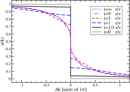
Figure 1: (color online) Time evolution of the momentum distribution $n_{t}(k)$ around the right Fermi point $k_{\mathrm{F}}>0$ ($\Delta k:=k-k_{\mathrm{F}}$) for the spinless TL-model with $\gamma=0.1$.

For $t=0$ in (6,7), $f(v,r)=1$ holds and the MD resulting from the Fourier transform of $e^{ik_{\mathrm{F}}x}/(2\pi(x+i0+))$ is the expected step function of the Fermi sea, cf.  Fig. 1. For $t=\infty$ we have $f(v,r)=r^{2}/(r^{2}+x^{2})$ which implies a power law $n(k)-1/2\propto\Delta k^{4\gamma(1+\gamma)}$ without a jump. Although a stationary correlation has been reached no thermalization has taken place because of the simplicity of the model: macroscopic number of conserved quantities, too little variation in the dispersion Cazalilla (2006); Barthel and Schollwöck (2008).

We focus on small and intermediate times for which we find that $G_{\mathrm{R}}(x,t)$ decreases always like $1/x$ which implies a finite jump at the Fermi vector. The time-dependent prefactor of $1/x$ is given by the first fraction $r^{2}/(r^{2}+(2vt)^{2})$ in (7) to the power $2\gamma(1+\gamma)$ which agrees for $t\to\infty$ with previous analyses Cazalilla (2006); Iucci and Cazalilla (2009). Hence there is a completely smooth decrease of the jump

$$\Delta n(t)=[r^{2}/(r^{2}+(2vt)^{2})]^{2\gamma(1+\gamma)},$$ (8)

remaining finite at all finite times. The complete MD at various times is obtained by numerical Fourier transformation; see Fig. 1. In the estimate $r/v\approx\hbar/J={\cal O}(1\mathrm{ms})$ $J$ is the hopping element from site to site which leads to the stated time scales for atoms in optical lattices Greiner et al. (2002); Bloch et al. (2008). The MD $n_{t}(k)$ at given $k$ does not evolve monotonically in time but displays oscillations in line with previous perturbative Moeckel and Kehrein (2008) and numerical Manmana et al. (2007) results.

Inspecting (5) it is obvious why the $1/x$ proportionality of $G_{\mathrm{R}}(x,t)$ does not change in the course of time. The operator $\varphi_{\mathrm{R}}(x,t)$ propagates through space at maximum with speed $v$. Hence there is no way how for a given time the long distance behavior is changed. This argument relies on the existence of a maximum speed $v_{\mathrm{max}}<\infty$ by which information can travel through the system. This phenomenon was called light-cone effect by Calabrese and Cardy Calabrese and Cardy (2006); they used the term for the propagation of entangled quasiparticles a quench. Note for later discussion that such a maximum speed generally exists independently of the system’s dimension.

But the prefactor of the $1/x$ correlation changes in time in spite of the light-cone effect. This represents a major change in the correlations. Inspecting our derivation we see that this effect stems from local commutators, i.e., from commutators between $\varphi_{\alpha}(x\pm vt)$ and $\varphi_{\alpha}^{\dagger}(x\mp vt)$ or from the corresponding pair at $x=0$. Thus there is a multiplicative renormalization of the matrix element which links $\hat{\psi}^{\dagger}(x,t)_{\mathrm{R}}|0\rangle$ to $\hat{\psi}^{\dagger}(x)_{\mathrm{R}}|0\rangle$. Below we show that this is also the generic situation in higher dimensions. Here we point out that for the behavior over short distances and short times the TL model is not special. All corrections which might be induced by other terms, which are present in more general models, will not change the qualitative behavior found here because they can be treated for short distances and times perturbatively.

For completeness we wish to extend the results for the spinless TL model to its counterpart with spin where charge ($\mathrm{c}$) and spin ($\mathrm{s}$) bosonic operators arise from the symmetric and antisymmetric, respectively, combination of the $\uparrow$ and $\downarrow$ bosonic operators Meden and Schönhammer (1992); Voit (1995). The Hamiltonian is diagonal in charge and spin bosons. It is characterized by the charge triple $v_{\mathrm{c}},r_{\mathrm{c}},\gamma_{\mathrm{c}}$ and the spin triple $v_{\mathrm{s}},r_{\mathrm{s}},\gamma_{\mathrm{s}}$. In the extended boson identity (4) the sum of the charge $\varphi_{\mathrm{R,c}}$ and the spin $\varphi_{\mathrm{R,s}}$ modes occur multiplied by $1/\sqrt{2}$ due to normalization Meden and Schönhammer (1992). Pursuing the same manipulations as in the spinless case eventually leads to

$$G_{\mathrm{R}}(x,t)=\frac{e^{ik_{\mathrm{F}}x}}{2\pi(x+ia)}f(v_{\mathrm{c}},r_{\mathrm{c}})^{\gamma_{\mathrm{c}}(1+\gamma_{\mathrm{c}})}f(v_{\mathrm{s}},r_{\mathrm{s}})^{\gamma_{\mathrm{s}}(1+\gamma_{\mathrm{s}})}.$$ (9)

On the one hand, many qualitative features are the same as in the spinless case, in particular the persistence of a finite jump in the MD for all times. It is given by

$$\Delta n(t)=\Big{[}\frac{r_{\mathrm{c}}^{2}}{r_{\mathrm{c}}^{2}+(2v_{\mathrm{c}}t)^{2}}\Big{]}^{\gamma_{\mathrm{c}}(1+\gamma_{\mathrm{c}})}\Big{[}\frac{r_{\mathrm{s}}^{2}}{r_{\mathrm{s}}^{2}+(2v_{\mathrm{s}}t)^{2}}\Big{]}^{\gamma_{\mathrm{s}}(1+\gamma_{\mathrm{s}})}.$$ (10)

On the other hand, the appearance of two velocities, two length scales and two exponents which are possibly different leads to a richer phenomenology. We refrain from showing explicit results because the MDs look very similar to the ones in Fig. 1. The difference in the decrease with the distance $x$ between Eqs. (6) and (9) is hardly discernible. Hence spin-charge separation, i.e., the difference $v_{\mathrm{c}}\neq v_{\mathrm{s}}$ is visible only in high precision measurements.

General Interacting Fermions

Because the scattering induced by interaction is particularly strong in 1D, the persistence of the MD jump in 1D indicates that it should persist in higher dimensions as well. Alternatively, one may presume the persistence of the jump to be peculiar to 1D. To support our view that the persistence is generic we will analyze the general equations of motion below. Note that in all dimensions a maximum speed $v_{\mathrm{max}}<\infty$ exists at which operators can propagate. Thus the long range behavior of correlations cannot change within a finite times.

To be specific we consider the 1-particle correlation $G(\mathbf{r},t)=-i\langle 0|\hat{\psi}(\mathbf{r},t)\hat{\psi}^{\dagger}(\mathbf{0},t)|0\rangle$ where the Heisenberg time evolution of the operators is induced by the interacting Hamiltonian $H$ while $|0\rangle$ is the Fermi sea of the noninteracting Hamiltonian $H_{0}$. A spin dependence is omitted for simplicity. The Heisenberg equation reads $\partial_{t}\hat{\psi}^{\dagger}(\mathbf{r},t)=i[H,\hat{\psi}^{\dagger}(\mathbf{r},t)]$. The commutation with $H_{0}$ (Liouville operator $L_{0}$) will propagate the 1-particle operator only. The commutation with the interaction ($L_{\mathrm{I}}$) generates a particle-hole (PH) pair. The iteration of $L_{\mathrm{I}}$ increases the number of particle-hole pairs. Hence the structure of the solution is

$$\hat{\psi}^{\dagger}(\mathbf{r},t)=P^{\dagger}_{\mathbf{r}}+P^{\dagger}(P^{\dagger}H^{\dagger})_{\mathbf{r}}+P^{\dagger}(P^{\dagger}H^{\dagger})^{2}_{\mathbf{r}}+\ldots$$ (11)

where $P^{\dagger}$ ($H^{\dagger}$) stands for a created particle (hole). It is understood that each term in (11) is normal-ordered relative to the Fermi sea $|0\rangle$. The application $L_{0}$ will reproduce the structure of a term $P^{\dagger}(P^{\dagger}H^{\dagger})^{m}_{\mathbf{r}}$, i.e., $m$ stays fixed, while $L_{\mathrm{I}}$ can increase $m$ by one, leave it unchanged, decrease it by one or by two. The first two terms in (11) are denoted explicitly in $d$ dimensions

$$P^{\dagger}_{\mathbf{r}}=\int_{|\mathbf{r}_{1}|<v_{\mathrm{max}}t}h_{0}(\mathbf{r}_{1},t):\hat{\psi}^{\dagger}(\mathbf{r}_{1}+\mathbf{r}):d^{d}r_{1}$$ (12)

$$P^{\dagger}(P^{\dagger}H^{\dagger})_{\mathbf{r}}=\iiint_{|\mathbf{r}_{j}|<v_{\mathrm{max}}t}h_{1}(\mathbf{r}_{1},\mathbf{r}_{2},\mathbf{r}_{3},t)\cdot$$

$$:\hat{\psi}^{\dagger}(\mathbf{r}_{1}+\mathbf{r})\hat{\psi}^{\dagger}(\mathbf{r}_{2}+\mathbf{r})\hat{\psi}(\mathbf{r}_{3}+\mathbf{r}):d^{d}r_{1}d^{d}r_{2}d^{d}r_{3}.\qquad$$ (13)

The Heisenberg equation generates a hierarchy of coupled differential equations for the $h_{m}(\{\mathbf{r}_{j}\},t)$. Because $h_{m}(\{\mathbf{r}_{j}\},0)=0$ for $m>0$ and a term with $m$ PH pairs requires at least $m$ applications of $L_{\mathrm{I}}$ we know $h_{m}={\cal O}((Ut)^{m})$ where $U$ is a generic value of the interaction. The expansion in $t$ can be computed order by order. Though we cannot prove the convergence of the series $t$ we do not see any means that the radius of convergence vanishes for Hamiltonians with finite coefficients. Certainly, the hierarchy is finite and thus well-behaved if calculations up to a finite order in the interaction, e.g., $U^{4}$, are carried out.

For $G(\mathbf{r},t)$ the expectation value $\langle 0|\hat{\psi}(\mathbf{r},t)\hat{\psi}^{\dagger}(\mathbf{0},t)|0\rangle$ must be evaluated which contains terms like

$$\langle 0|(HP)^{m}P_{\mathbf{r}}^{\phantom{j}}P^{\dagger}(P^{\dagger}H^{\dagger})^{j}_{\mathbf{0}}\rangle=\delta_{m,j}G^{(2m+1)}(\mathbf{r},t)$$ (14)

because only states with the same number of PH pairs can have a finite overlap. The Wick theorem is applicable because $|0\rangle$ is a Fermi sea so that the many-particle correlations can be reduced to products of the initial 1-particle correlations $g(\mathbf{r}):=G(\mathbf{r},0)$. Thus we know $G^{(2m+1)}(\mathbf{r},t)={\cal O}\left(g(\mathbf{r})^{2m+1}\right)$. The information about the jump is encoded in the most slowly decreasing contribution for $|\mathbf{r}|\to\infty$, namely the one for $m=0$

$$G^{(1)}(\mathbf{r},t) = \iint_{|\mathbf{r}_{j}|<v_{\mathrm{max}}t}h_{0}^{*}(\mathbf{r}_{1},t)\cdot$$ (15)

$$g(\mathbf{r}+\mathbf{r}_{1}-\mathbf{r}_{2})h_{0}(\mathbf{r}_{2},t)d^{d}r_{1}d^{d}r_{2}.\qquad$$

This double convolution implies $n_{t}^{(1)}(\mathbf{k})=n_{0}(\mathbf{k})|h_{0}(\mathbf{k},t)|^{2}$ in momentum space where $n_{0}(\mathbf{k})\in\{0,1\}$ is the noninteracting MD. Clearly, the nonequilibrium 1-particle correlations inherit many of their qualitative properties from the 1-particle correlations before the quench. Interestingly, the jumps in the MD occur at the same loci where the noninteracting MD $n_{0}(\mathbf{k})$ jumps, i.e., at the noninteracting Fermi surface FS₀. The reduction of the jump is given by

$$\Delta n(t)\big{|}_{\mathbf{k}\in\mathrm{FS}_{0}}=|h_{0}(\mathbf{k},t)|^{2}\big{|}_{\mathbf{k}\in\mathrm{FS}_{0}}.$$ (16)

The Fourier transform $h_{0}(\mathbf{k},t)$ corresponds exactly to $h_{k\uparrow}$ in Ref. Moeckel and Kehrein, 2008 after the forward-backward CUT. These general equations set the stage for the analysis of higher dimensional systems and allow us to draw general conclusions. Further analysis has to be numerical and it is therefore left to future research.

Conclusions

Summarizing, we studied interaction quenches of noninteracting Fermi gases. The focus was the question how the jump in the momentum distribution (MD) vanishes. In 1D the Tomonaga-Luttinger model was investigated quantitatively and in higher dimension the general equations of motions were set up. For generic Hamiltonians without diverging coefficients we showed that the jump survives for small and intermediate times, displaying a smooth behavior as function of time. If thermalization takes place, we expect that the jump decreases exponentially (with or without oscillations).

We found that the quenched MD still displays many qualitative features of the noninteracting Fermi sea. In particular, the loci of the jumps are those of the Fermi sea. The Fermi surface of isolated quenched interacting fermion models does not evolve at all. The models have to be extended in order to incorporate relaxation of the Fermi surface geometry. Finally, we point out that the approach used here for the general situation can also be extended to correlations of two or more particles.

We gratefully acknowledge many helpful discussions with F.B. Anders and S. Kehrein.

References

- Bloch et al. (2008) I. Bloch, J. Dalibard, and W. Zwerger, Rev. Mod. Phys. 80, 885 (2008).
- Greiner et al. (2002) M. Greiner, O. Mandel, T. W. Hänsch, and I. Bloch, Nature 415, 39 (2002).
- Perfetti et al. (2006) L. Perfetti, P. A. Loukakos, M. Lisowski, U. Bovensiepen, H. Berger, S. Biermann, P. S. Cornaglia, A. Georges, and M. Wolf, Phys. Rev. Lett. 97, 067402 (2006).
- White and Feiguin (2004) S. R. White and A. E. Feiguin, Phys. Rev. Lett. 93, 076401 (2004).
- Daley et al. (2004) A. J. Daley, C. Kollath, U. Schollwöck, and G. Vidal, J. Stat. Mech.: Theor. Exp. p. P04005 (2004).
- Anders and Schiller (2005) F. B. Anders and A. Schiller, Phys. Rev. Lett. 95, 196801 (2005); Phys. Rev. B 74, 245113 (2006).
- Freericks et al. (2006) J. K. Freericks, V. M. Turkowski, and V. Zlatić, Phys. Rev. Lett. 97, 266408 (2006).
- Eckstein and Kollar (2008) M. Eckstein and M. Kollar, Phys. Rev. Lett. 100, 120404 (2008).
- Eckstein et al. (2009) M. Eckstein, M. Kollar, and P. Werner, Phys. Rev. Lett. 103, 056403 (2009).
- Moeckel and Kehrein (2008) M. Moeckel and S. Kehrein, Phys. Rev. Lett. 100, 175702 (2008); Ann. Phys. 324, 2146 (2009).
- Rigol et al. (2007) M. Rigol, V. Dunjko, V. Yurovsky, and M. Olshanii, Phys. Rev. Lett. 98, 050405 (2007).
- Gangardt and Pustilnik (2008) D. M. Gangardt and M. Pustilnik, Phys. Rev. A 77, 041604(R) (2008).
- Calabrese and Cardy (2006) P. Calabrese and J. Cardy, Phys. Rev. Lett. 96, 136801 (2006).
- Cazalilla (2006) M. A. Cazalilla, Phys. Rev. Lett. 97, 156403 (2006).
- Barthel and Schollwöck (2008) T. Barthel and U. Schollwöck, Phys. Rev. Lett. 100, 100601 (2008).
- Kollath et al. (2007) C. Kollath, A. M. Läuchli, and E. Altman, Phys. Rev. Lett. 98, 180601 (2007).
- Manmana et al. (2007) S. R. Manmana, S. Wessel, R. M. Noack, and A. Muramatsu, Phys. Rev. Lett. 98, 210405 (2007).
- Rigol et al. (2008) M. Rigol, V. Dunjko, and M. Olshanii, Nature 452, 854 (2008).
- Iucci and Cazalilla (2009) A. Iucci and M. A. Cazalilla, arXiv:0903.1205 (2009).
- Meden and Schönhammer (1992) V. Meden and K. Schönhammer, Phys. Rev. B 46, 15753 (1992).
- Voit (1995) J. Voit, Rep. Prog. Phys. 58, 977 (1995).
- von Delft and Schoeller (1998) J. von Delft and H. Schoeller, Ann. Physik 7, 225 (1998).
- Uhrig (2004) G. S. Uhrig, Lecture Notes available at t1.physik.tu-dortmund.de/uhrig/liquids_ss2004.html.
- Luther and Peschel (1974) A. Luther and I. Peschel, Phys. Rev. B 9, 2911 (1974).