Prospects for the Measurement of the Unitarity Triangle Angle from Decays
Abstract
The potential for a precise measurement of the Unitarity Triangle angle in future experiments from the decay is well-known. It has recently been suggested that the sensitivity can be significantly enhanced by analysing the Dalitz plot to extract amplitudes relative to those of the flavour-specific decay . An extension to this method which includes the case where the neutral meson is reconstructed in suppressed final states is presented. The sensitivity to is estimated using this method and compared to that obtained using the decay alone. Experimental effects, such as background contamination, are also considered. This approach appears to be a highly attractive addition to the family of methods that can be used to determine .
pacs:
13.25.Hw, 12.15.Hh, 11.30.ErI Introduction
The quark flavour sector of the Standard Model of particle physics, described by the Cabibbo-Kobayashi-Maskawa (CKM) quark mixing matrix Cabibbo:1963yz ; Kobayashi:1973fv , gives a successful description of all current experimental measurements of quark flavour-changing interactions. It also provides an excellent laboratory to search for effects of physics beyond the Standard Model (see, for example, Refs. Buchalla:2008jp ; Browder:2008em ; Antonelli:2009ws ). A critical element of this programme is the precise measurement of the angle of the Unitarity Triangle formed from elements of the CKM matrix.
A method to measure with negligible theoretical uncertainty was proposed by Gronau, London and Wyler (GLW) Gronau:1990ra ; Gronau:1991dp . The original method uses decays, with the neutral meson reconstructed in eigenstates. The method can be extended to use meson decays to any final state that is accessible to both and , in particular doubly-Cabibbo-suppressed decays such as Atwood:1996ci ; Atwood:2000ck have been noted to provide enhanced sensitivity to -violation effects.
The use of neutral decays is particularly interesting since the two contributing amplitudes are more similar in magnitude, so that direct -violation effects may be enhanced relative to those in charged decays. The decay is especially advantageous since the charge of the kaon in the decay unambiguously tags the flavour of the decaying meson, obviating the need for time-dependent analysis Dunietz:1991yd . This appears to be one of the most promising channels for LHCb to make a precise measurement of Akiba:2007zz ; Akiba:2008zz ; Nardulli:2008 .
The approach that has mainly been considered until recently is a quasi-two-body analysis of . In this analysis, the contributions from other resonances in the Dalitz plot that interfere with the within the selected mass window are handled by the introduction of an additional hadronic parameter Gronau:2002mu . This parameter, normally denoted by , takes values between 0 and 1 where 0 implies that all sensitivity to is lost, and the limit of 1 is reached in the case that no amplitudes other than contribute. Estimates suggest that for a mass window of Pruvot:2007yd .
Recently it has been noted that the natural width of the meson can be used to enhance the sensitivity to the -violating phase through analysis of the Dalitz plots Bediaga ; Gershon:2008pe . By comparison of the Dalitz-plot distributions of events in the cases where the neutral meson is reconstructed in flavour-specific and -eigenstate modes, the complex amplitudes of the decays can each be determined relative to the flavour-specific amplitude. This allows for a direct extraction of from the difference in amplitudes, rather than from the rates.
In this paper we extend the method proposed in Ref. Gershon:2008pe to include also the case where the neutral meson is reconstructed in suppressed final states. This allows us to make a direct comparison of the sensitivity to between the quasi-two-body analysis and the Dalitz-plot analysis. We also study possible systematic effects that may limit the sensitivity of the analysis, including uncertainties on the correct composition of the Dalitz-plot model and a brief discussion of experimental effects.
The remainder of the paper is organised as follows: in Section II we give an overview of the method; in Section III we describe the Dalitz-plot model used for our study; in Sections IV and V we present the results we obtain in the quasi-two-body analysis and in the Dalitz-plot analysis, respectively; in Section VI we discuss how experimental effects can be handled, before summarising in Section VII.
II Method
In this Section we describe the various methods that can be used to extract from . We first review the quasi-two-body approach, and then recap the recently proposed Dalitz-plot technique Gershon:2008pe , before describing the extension to the method used in our study. All methods exploit the interference between the two tree-level amplitudes shown in Fig. 1. Conventionally, the ratio of magnitudes of these two amplitudes is referred to as , while their strong phase difference is labelled .
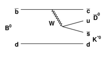
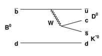
The GLW method Gronau:1990ra ; Gronau:1991dp of extracting uses the following rates and asymmetries in decays:
| (1) | |||||
| (2) | |||||
Here, () is used to refer to either or ( or ), while refers to a neutral meson reconstructed in a -even (eg. ) or -odd (eg. ) final state, and refers to a neutral meson reconstructed in a favoured, quasi-flavour-specific (eg. ) final state. Note that experimentally it is convenient to measure normalised to an equivalent double ratio from or decays.
Since , the above four observables give three independent constraints on the three parameters , and . This is sufficient to solve the system up to an eightfold ambiguity. However, when measurements are performed in a hadronic environment as at LHCb, the reconstruction of the -odd final states becomes a significant experimental problem. Therefore, additional observables are required.
A solution is to include doubly-Cabibbo-suppressed meson decays, as first suggested by Atwood, Dunietz and Soni (ADS) Atwood:1996ci ; Atwood:2000ck . Due to the fact that the meson decays to are not truly flavour-specific, but include a suppressed contribution which is given by relative to the favoured decay amplitude,111 Note that the sign convention for used in this paper is opposite to that used in most of the literature on measurements. enhanced -violation effects can occur. The rates and asymmetries of the decays to the suppressed final states are then given by
| (3) | |||||
| (4) | |||||
Since the hadronic parameters of the decay ( and ) can be determined independently Rosner:2008fq ; Asner:2008ft , these measurements provide two additional linearly independent constraints that can be used in combination with the GLW observables to obtain bounds on the three unknown parameters , and . With the decay modes , the ADS observables are well suited to reconstruction in a hadronic environment. Consequently, one of the most promising strategies for the tree-level determination of at LHCb is that from the combination of measurements of , , and in charged decays LHCb-2009-011 or neutral decays Akiba:2007zz ; Nardulli:2008 .
The finite width of the resonance leads to additional complications in the analysis of decays, since other contributions to the Dalitz plot can affect the population within the mass window. This can be handled by making the following substitutions Gronau:2002mu :
| (5) | |||||
| (6) |
where and are respectively the amplitudes carrying the phase of the (Fig. 1(left)) and of the (Fig. 1(right)) transitions, and is the strong phase difference between them, all as functions of the Dalitz-plot position . The integrals are over the region of the Dalitz plot that is defined as the mass window. In the limit that is the only contribution in this window, , and .
With this treatment, the two hadronic parameters associated with the decay ( and ) are replaced with two effective parameters ( and ) and a new unknown () is introduced. Since the combination of (-even) GLW and ADS observables provides four linearly independent measurements, it is possible to determine from the data together with , and . Alternatively, external input, either theoretical or experimental, could be used to constrain Pruvot:2007yd .
We refer to the extraction of using the approach outlined above as the quasi-two-body analysis. The addition of ADS observables helps to resolve two of the ambiguities of the GLW approach Soffer:1999dz ; however, the effectiveness of this depends on the values of , and , as well as the statistical sensitivity. Moreover, the sensitivity to depends on the values of the unknown hadronic parameters, particularly .
The recently proposed Dalitz-plot analysis Gershon:2008pe exploits the presence of the contribution that serves as a reference amplitude, since the flavour of the neutral meson produced in is tagged by the charge of the accompanying pion. Considering flavour-specific mesons, we can define the amplitude relative to this reference, as illustrated in Fig. 2(left),
| (7) |
Note that in Eq. 7 and throughout the discussion below we neglect factors of and that formally should appear in the numerator and denominator respectively, since they eventually cancel in the observables of interest.
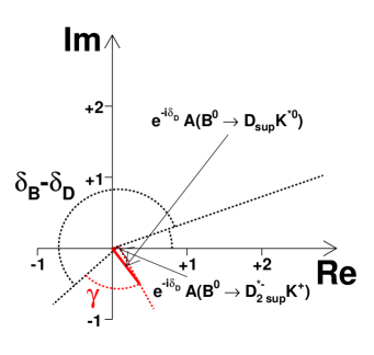
Considering now -even mesons, using the convention , we find (see Fig. 2(right))
| (8) |
where denotes that the neutral meson produced in the decay of the is reconstructed in a -even eigenstate. Thus, we find Gershon:2008pe
| (9) | |||||
where the variables are the same as those used in the analysis of with decays Poluektov:2006ia ; Aubert:2008bd . Constraints on are likewise obtained from equivalent expressions for the charge-conjugate decays. The extraction of from this Dalitz-plot analysis with only a single unresolvable ambiguity () is possible using only -even decays. Consequently, we restrict our discussion to -even decays, since those are experimentally accessible in a hadronic environment; however, we note that -odd decays give similar expressions, but with the right-hand side of the last two relations of Eq. 9 multiplied by a minus sign.
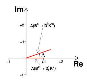
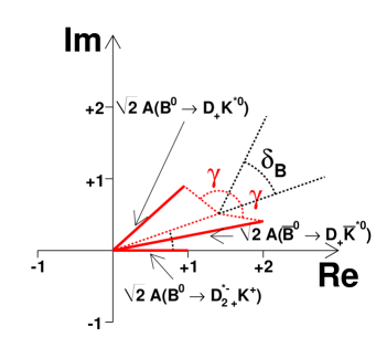
The discussion above, and in Ref. Gershon:2008pe , considers that the mesons used for normalisation are reconstructed in flavour-specific final states. However, as already mentioned, the favoured decay is only approximately flavour-specific. Furthermore, since the doubly-Cabibbo-suppressed decays are used to great benefit in the quasi-two-body analysis, it is reasonable to ask if they can also be included in the Dalitz-plot analysis. We therefore extend the method to include the effects of the suppressed -decay amplitudes. We find
while the expression for the amplitude ratio in the Dalitz plot with the -even meson is unchanged from Eq. 8. These amplitudes are illustrated in Fig. 3. As before, the equivalent expressions for the charge-conjugate decays are obtained with the substitution .
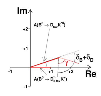
As one would expect, the amplitudes obtained from the Dalitz plot (Fig. 3(left)) are hardly distinguishable from those for the idealised flavour-specific decays. As discussed in Ref. Gershon:2008pe , if the suppressed amplitudes are neglected, it will lead to only a small bias in the extraction of .
The amplitudes obtained from the Dalitz plot (Fig. 3(right)) are markedly different from those of the other Dalitz plots, and this new information can in principle be used to constrain . However, in this case the contribution is no longer suitable as a reference amplitude, due to its small size, and the measurement of the relative phase between and amplitudes would be expected to have a large uncertainty. Nonetheless, it should be possible to obtain information about the relative magnitude of these amplitudes, which will provide sensitivity to . Note that, in contrast to the quasi-two-body analysis, it is not necessary to use external constraints on and in the Dalitz-plot analysis.
III Dalitz Plot Model
We construct a model for Dalitz plot distributions using the isobar formalism, in which the total amplitude is written as the coherent sum of contributions from resonant and nonresonant terms:
In Eq. III, represents the position in the Dalitz plot, describes the complex amplitude for each component, the terms denote vertex form factors, the resonance propagator and the Lorentz invariant spin factor. We use Blatt-Weisskopf barrier form factors Blatt , and use relativistic Breit-Wigner lineshapes to describe the propagators. We use the Zemach formalism Zemach:1963bc ; Zemach:1968zz for the spin factors. We assume that the nonresonant contribution is constant across the phase space. This is a sufficient approximation for the study at hand, even though a more complicated description is likely to be necessary to fit real data. All amplitudes are evaluated using the qft++ package Williams:2008wu .
We develop a model for the Dalitz plot distribution based on the following results from Ref. Aubert:2005yt :
The results for the resonant contributions were extracted using events in the regions MeV and MeV, respectively. The strengths of the and amplitudes in our model were set by requiring that the fit fractions of these resonances in these regions match the published results Aubert:2005yt .
Since we expect the Dalitz plot to contain contributions from other resonances not considered in Ref. Aubert:2005yt , we add additional contributions based on results from an analysis of the Dalitz plot Aubert:2007qe , taking isospin and colour-suppression factors into account as appropriate. Some additional scaling of these resonance terms was performed to provide a better match to the results published in Ref. Aubert:2005yt . These experimental results provide information about the likely magnitude of contributions from and resonances to the Dalitz plot.
Additionally, contributions from -type resonances can in principle contribute. Their effect could be significant since they are mediated by transitions which provide the sensitivity to . The and states are known to decay to , and the latter has been observed in decays :2007aa . These are not included in our nominal model, but we consider their potential effect among the model variations discussed below in Section V.
| Resonance | Mass (MeV) | Width (MeV) | |
|---|---|---|---|
| 896 | 51 | ||
| 1412 | 294 | ||
| 1432 | 109 | ||
| 1717 | 322 | ||
| 2403 | 283 | ||
| 2459 | 25 | ||
| 2690 | 110 |
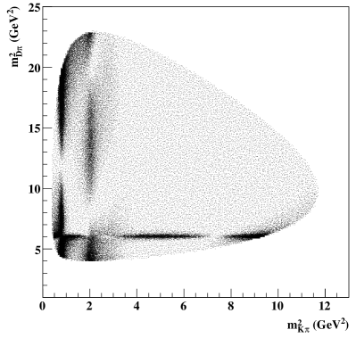
Table 1 summarises the parameters of the resonances used in our analysis. Table 2 gives the fit fractions and relative phases of the various intermediate states that contribute to our Dalitz plot model. The parameters given are appropriate for the case that the neutral meson decays to a favoured, quasi-flavour-specific final state (namely, , and charge conjugate). An example Dalitz-plot distribution generated from this model is shown in Fig. 4.
We derive the Dalitz-plot distributions for other -decay final states using the equations presented in Section II and initially taking . We consider several different possible values of and for the amplitudes, while for the less significant contributions from other channels we simply set and . We note that our nominal value of is at the upper end of the experimentally allowed range for this parameter (e.g. the UTfit Collaboration gives at confidence level Bona:2006ah ), but it is convenient to use this value to allow comparison with previous studies.
| Intermediate state | Fit fraction | Phase (∘) |
|---|---|---|
| 0.46 | 0 | |
| 0.0001 | 284 | |
| 0.12 | 221 | |
| 0.02 | 128 | |
| 0.34 | 325 | |
| 0.02 | 267 | |
| nonresonant | 0.06 | 140 |
We use our Dalitz-plot model to generate ensembles of event samples corresponding to the different meson final states. The numbers of events are based on expectations for one year of nominal luminosity at LHCb () Akiba:2008zz , assuming that the efficiency does not vary across the Dalitz plot. The exact numbers in each sample vary as functions of the input values of the parameters (particularly and ), but typically are around 7300 for , 700 for and 600 for (for and decays combined).
IV Results with the Quasi-two-body Approach
We first study the sensitivity to in the quasi-two-body approach. We take the six Dalitz-plot distributions (, and all for both and ) generated as described in the previous section, and apply selection requirements to select the dominated region. We then perform minimisation to fit the yields in each sample to determine five parameters: and an overall normalisation. The parameters and are fixed to their measured values ( and , respectively). For each pseudo-experiment we perform ten fits with initial values of the parameters randomised in the ranges , , , , and we take the results of the fit with the smallest .
The selection requirements for the are an interesting sub-topic worthy of some discussion. The width of the invariant-mass window around the nominal mass affects the size of the event samples. Increasing the width yields greater statistics so that one would naïvely expect a reduction in the statistical uncertainty on . Unfortunately, increasing the width of the invariant-mass window also leads to an increase in the dilution from the non- component of the amplitude, i.e. a decrease in , which tends to decrease the sensitivity to . Hence, it is important to optimise the selection requirements.
One can increase by introducing a veto (e.g. rejecting events that satisfy ). This veto has a rather minimal impact on the statistics. In our nominal model with , choosing to use yields . Applying the veto above increases this to . Decreasing the invariant-mass window to yields ; however, with the limited statistics in our pseudo-experiments, this decrease in dilution is counter-balanced by the loss of statistics. Experiments with higher statistics may benefit by using a tighter invariant-mass window. In the results below, we proceed using the veto discussed above and requiring the invariant mass to be within 150 MeV of the nominal mass.
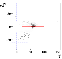
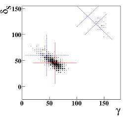
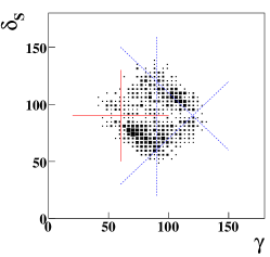
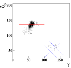
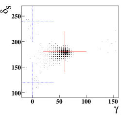
Results from the pseudo-experiments for various different input values of are shown in Fig. 5. It is apparent that there is a strong correlation between the fitted values of and , and moreover that there are ambiguities in the solution that are particularly pronounced for values of near . The locations of each of the ambiguous solutions for the case where are also shown in Fig. 5. The ambiguities in the solutions found by fitting our data are close to these values. Since is small (our data were generated with ), statistical fluctuations can lead to the best value being obtained near one of the ambiguous solutions. The inability to resolve such ambiguities is a limitation of the quasi-two-body method.
As a consequence of these ambiguities, the distributions of the fitted values of are not Gaussian. Therefore, in Tab. 3, we report both the mean and rms of each distribution as well as the corresponding values obtained by fitting the data in the regions near the generated values of to Gaussian lineshapes, i.e. ignoring the ambiguities in the solution. For , it is not possible to separate the correct solutions from the ambiguous solution, so we have not performed a Gaussian fit to the distributions for this sample.
We have also considered an alternative approach to the fits, in which the value of is fixed. Although can only be measured from analysis of Dalitz plots (so that if this measurement can be performed, the Dalitz plot analysis will most likely be feasible), it is conceivable that may be determined from theory, or from a different experiment. We therefore repeat the fits with constrained to the values obtained directly from our model. This approach leads to an improvement in the resolution on near some solutions (e.g., near the true solution for ), but does not remove the ambiguities (see Fig. 6). The results obtained by fitting the regions near the generated values of to Gaussian lineshapes can be found in Tab. 3. This provides a comparison with Ref. Akiba:2008zz , where the same approach was used to estimate the sensitivity to using the quasi-two-body approach on one nominal year’s data from LHCb. Despite several important differences between our toy study and the detailed sensitivity study of Ref. Akiba:2008zz , the results are in very good agreement (see Tab. 3). This provides confidence in the absolute scale of our sensitivity estimates.
| (∘) | |||||||
| free | locked | Ref. Akiba:2008zz | |||||
| Distribution | Gaussian fit | Gaussian fit | |||||
| mean | rms | ||||||
| 55.5 | 14.6 | 57.7 | 7.3 | 60.1 | 5.9 | 6.2 | |
| 60.2 | 19.6 | 57.4 | 10.6 | 57.8 | 10.3 | 10.8 | |
| 88.3 | 17.9 | 12.7 | |||||
| 60.4 | 18.0 | 56.6 | 9.4 | 56.3 | 9.7 | 9.5 | |
| 55.1 | 19.2 | 56.6 | 7.4 | 59.7 | 5.5 | 5.2 | |
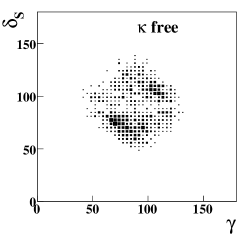
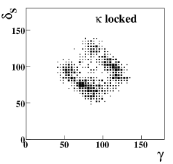
The results obtained by varying in our model are given in Tab. 4. As is well known, the sensitivity to reduces as becomes smaller. It is also clear that the effect of ambiguities becomes more significant, since the discrepancy between the rms of the whole distributions and the width of the Gaussian peak near the correct solution increases.
| (∘) | ||||
|---|---|---|---|---|
| Distribution | Gaussian fit | |||
| mean | rms | |||
| 55.5 | 14.6 | 57.7 | 7.3 | |
| 57.0 | 21.1 | 56.8 | 9.7 | |
| 58.9 | 29.3 | 56.9 | 11.8 | |
V Results with the Amplitude Analysis
To study the sensitivity to using the Dalitz-plot analysis, we perform a simultaneous maximum likelihood fit to all six Dalitz-plot distributions. We initially fix and to their measured values, leaving 24 free parameters (, four parameters – , , & – for each -type resonance and nonresonant contribution, and two – magnitude and phase – for each -type resonance, with one phase fixed). As before, for each pseudo-experiment we perform multiple fits with randomised initial parameter values, and we take the results of the fit with the smallest negative log-likelihood.
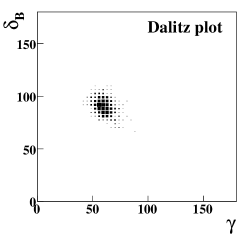
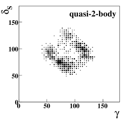
In Section IV, we found that the quasi-two-body approach was, in many cases, unable to resolve ambiguities in the solution. This was especially true for values of near . Figure 7 shows the distributions of results from the pseudo-experiments generated with for the amplitude and quasi-two-body approaches. The additional information utilised in the amplitude analysis is sufficient to remove the ambiguities in the solution.
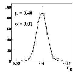
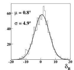
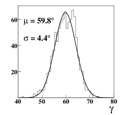
The distributions of the fit results for the parameters , and obtained from the pseudo-experiments generated with are shown in Fig. 8. We fit the distributions with Gaussian lineshapes, since all are consistent with this shape (this is true for all values), and report the means and widths in Tab. 5. The resolution on varies between , depending on the value of , in our nominal model. Thus, unlike for the quasi-two-body approach (Tab. 3), the sensitivity to is not strongly dependent on the value of .
| (∘) | (∘) | |||||
|---|---|---|---|---|---|---|
| 0.40 | 0.01 | 0.8 | 4.9 | 59.8 | 4.4 | |
| 0.40 | 0.01 | 46.2 | 6.0 | 59.2 | 5.5 | |
| 0.40 | 0.01 | 90.2 | 6.4 | 59.8 | 5.7 | |
| 0.40 | 0.01 | 134.0 | 6.3 | 59.3 | 5.8 | |
| 0.40 | 0.01 | 179.8 | 4.2 | 59.7 | 4.2 | |
The physical values of and may be different from those used in our model. To study how this would affect our results, we vary the values of and in our model and fit the data using the same procedure outlined above. The results obtained considering are given in Tab. 6. As expected, the sensitivity to decreases as decreases; however, even for the distribution of fit results is still approximately Gaussian, and the resolution on is still . The results obtained considering are given in Tab. 7. We conclude that the sensitivity to does not depend strongly on the value of itself.
| (∘) | (∘) | |||||
|---|---|---|---|---|---|---|
| 0.40 | 0.01 | 0.8 | 4.9 | 59.8 | 4.4 | |
| 0.30 | 0.01 | 0.7 | 5.9 | 60.0 | 5.3 | |
| 0.20 | 0.01 | 0.6 | 7.0 | 59.5 | 7.0 | |
| (∘) | (∘) | |||||
|---|---|---|---|---|---|---|
| 0.40 | 0.01 | 1.2 | 6.0 | 44.6 | 5.2 | |
| 0.40 | 0.01 | 0.8 | 4.9 | 59.8 | 4.4 | |
| 0.40 | 0.01 | 0.4 | 4.5 | 74.8 | 4.0 | |
There are a number of parameters in our model which are not well constrained by data; however, most of these are not expected to impact significantly the sensitivity to . For example, the strong phase between the and amplitudes, which we denote by , could be very different from the value used in our model. To determine what effect the value of this parameter has on the extracted value of , we vary in our model over the physically allowed range, , and refit the data. The fit results, given in Tab. 8, show that the impact on the sensitivity to is minimal.
| (∘) | (∘) | |||||
|---|---|---|---|---|---|---|
| 0.40 | 0.01 | 0.5 | 4.9 | 59.7 | 4.1 | |
| 0.40 | 0.01 | 0.4 | 4.9 | 59.7 | 4.3 | |
| 0.40 | 0.01 | 0.0 | 5.0 | 59.5 | 4.0 | |
| 0.40 | 0.01 | 0.8 | 4.9 | 59.8 | 4.4 | |
None of the parameters for the , or amplitudes is well constrained by data. To see what effect the presence of violation in these amplitudes has on the sensitivity to , we set , and in our model and refit the data. The results obtained for this model variation are given in Tab. 9. There is no appreciable bias on the extracted value of , and the resolution on decreases by only . This is not surprising given the relatively small contributions to the total amplitude from , and (see Tab. 2). If, however, in real data these or any other -type amplitudes do contribute strongly to (and have sufficiently large violation), then the sensitivity to could be better than that obtained from our nominal model. To further test how mismodelling of the Dalitz plot may affect the extracted value of , we refit the data from our nominal model using only the , and nonresonant amplitudes (fixing all others to zero). The results are shown in Tab. 10. Again, there is little impact on the extracted values, indicating that this analysis may suffer much less model-related uncertainties than some other methods to extract Poluektov:2006ia ; Aubert:2008bd .
| (∘) | (∘) | ||||
| 0.40 | 0.01 | 0.1 | 5.2 | 59.0 | 5.6 |
| (∘) | (∘) | ||||
| 0.40 | 0.01 | -1.0 | 4.4 | 60.2 | 4.5 |
We have also tested how the addition of -type resonances may affect the analysis. We add to the model a contribution from , the magnitude of which is based on the assumption
| (13) |
The right-hand side of this expression is found to be for and for Amsler:2008zzb . Using results from Ref. :2007aa , we estimate
We add a contribution from this amplitude, with an arbitrary phase, to the model described in Tab. 2. The results of fits to pseudo-experiments generated with this modified model are summarised in Tab. 11. There is little or no improvement in the sensitivity to compared to the nominal model. This can be understood since the corner of the Dalitz plot where the and would interfere is excluded by kinematic constraints (see Fig. 4). Following this reasoning, larger effects from -type resonances would be possible if there were significant contributions to the Dalitz plot from heavier and/or heavier resonances.
| (∘) | (∘) | ||||
| 0.40 | 0.01 | 0.8 | 5.0 | 59.9 | 4.3 |
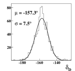
In our nominal fit, we fix the values of and . However, the value of is currently not precisely measured: Rosner:2008fq ; Asner:2008ft ; Barberio:2008fa . To study what effect this parameter can have on our results, we rerun the fits described above (on our nominal model) starting the value of randomly in the range . The results obtained for are shown in Fig. 9. The resolution extracted for is , which is less than the uncertainty on current measurements. Fitting with free has no significant effect on our results for , and (for all model values of ).
VI Experimental Effects
The study reported in the previous section neglected a number of experimental effects which will surely impact the sensitivity to in any real-world experiment. The effect most likely to have the largest impact on the resolution is the presence of background events. To study how this might affect the sensitivity to , we generate background events by sampling from a flat Dalitz distribution. For real data, there will almost certainly be some features present in the shape of the background; however, for our purposes, a flat background model should be sufficient. We take the expected background yields in each of the six final states to be equivalent. This should be a reasonable approximation provided the main source of background events is from combinatorics (a plausible assumption for LHCb). The ratio of background to signal, , is defined here as the ratio of the number of expected background events to the number of expected signal events for the final state with the smallest expected signal yield. We generate background events according to this prescription for the ratios and 100, and fit the data using the same procedure as in the previous section.
For , ambiguities in the solution begin to appear (see Fig. 10), just as they did using the quasi-two-body approach without background. About 2% of pseudo-experiments with find their best likelihood in an ambiguous solution. This number steadily increases as the background increases, reaching about 25% for . This can be understood since as the background increases, it becomes more difficult to extract cleanly the amplitudes with smaller contributions. The amplitude with the strongest contribution in our model is . Thus, in the presence of a large background contamination, the amplitude analysis essentially reduces to the quasi-two-body approach. This results in the ambiguities in the solution found in the quasi-two-body approach (without background) appearing in the amplitude analysis if the background yields are large.
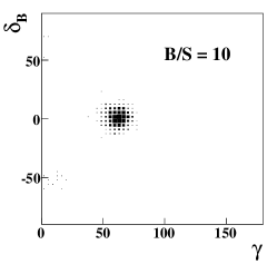
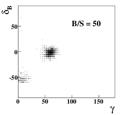
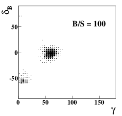
Our studies show that the background level should be kept to in order to take full advantage of the benefits of the amplitude analysis. This appears achievable, even in a hadronic environment. For the ambiguities in the solution still appear at the few percent level; however, one can study the likelihood contours to determine whether the solution for any given experiment may have ambiguities. The results obtained from an experiment with such a background would need to take this into account. Note also that these results are for a data sample roughly equivalent to one nominal year’s data taking at LHCb, and that effects due to ambiguities would be expected to be ameliorated with larger data samples.
The results obtained for , and are given in Tab. 12. The ambiguities in the solution discussed above have been ignored in these results, i.e. the means and widths for are obtained by fitting the region around the true solution to a Gaussian lineshape. The effects of the background on the resolution are minimal. The resolution of for is only worse than with no background. Even for the resolution is only about 60% worse. Thus, the most important impact of the presence of background events is their ability to lessen the power the amplitude analysis has to break the ambiguities found in the quasi-two-body analysis.
| (∘) | (∘) | |||||
|---|---|---|---|---|---|---|
| 0.40 | 0.01 | 0.8 | 4.9 | 59.8 | 4.4 | |
| 0.40 | 0.01 | 0.1 | 5.1 | 59.8 | 4.9 | |
| 0.39 | 0.01 | -0.8 | 5.2 | 61.0 | 5.0 | |
| 0.40 | 0.01 | 1.2 | 5.2 | 62.1 | 5.4 | |
| 0.40 | 0.01 | -1.5 | 5.8 | 59.5 | 6.2 | |
| 0.39 | 0.01 | -1.9 | 6.0 | 58.8 | 7.2 | |
Another experimental effect which must be taken into account in a real experimental analysis is the variation of reconstruction efficiency across the Dalitz plot. Our study has assumed that the efficiency is flat, but in reality one would expect the probability to reconstruct successfully a decay to be lower at the edges of phase space near the corners of the Dalitz plot. If the shape of the efficiency function is known, this can be taken into account in the analysis. However, systematic effects arise since the efficiency is typically measured using Monte Carlo simulations, which inevitably will not give exactly the same behaviour as the data.
It is impossible to give a quantitative estimate of how large an effect this may be. Nonetheless, there is a strong qualitative reason to believe that it will not be major problem. The key point is that the our amplitude analysis extracts from the difference between Dalitz-plot distributions with the meson reconstructed in different decay modes ( and eigenstates). Data/MC differences can be expected to cancel in the ratio of Dalitz-plot distributions, unless there is a momentum dependence in the ratio of efficiencies to reconstruct the meson in the different final states. Such an effect should be possible to study using control samples.
VII Summary
We have presented a feasibility study of an extension to the recently proposed method to extract the Unitarity Triangle angle from amplitude analysis of Dalitz plots. The analysis includes the cases where the neutral meson is reconstructed in -even eigenstates as well as in CKM-favoured and CKM-suppressed hadronic decays. Compared to the previously proposed quasi-two-body analysis, the amplitude analysis provides (i) at least better sensitivity to , (ii) resolution of ambiguous solutions, (iii) much reduced dependence of the sensitivity on the strong phase , and (iv) the possibility to determine the poorly known parameter . The analysis appears to be relatively robust against mismodelling of the Dalitz plot, and performs well even when relatively large backgrounds are present. We conclude that this method appears to be a highly attractive addition to the family of methods that can be used to determine .
We are grateful to our colleagues from the LHCb experiment, and would particularly like to thank Ignacio Bediaga, Alex Bondar, Ulrik Egede, Patrick Koppenburg, Anton Poluektov and Guy Wilkinson for discussions. This work is supported by the Science and Technology Facilities Council (United Kingdom).
References
- (1) N. Cabibbo, Phys. Rev. Lett. 10 (1963) 531.
- (2) M. Kobayashi and T. Maskawa, Prog. Theor. Phys. 49 (1973) 652.
- (3) M. Artuso et al., Eur. Phys. J. C 57 (2008) 309 [arXiv:0801.1833 [hep-ph]].
- (4) T.E. Browder, T. Gershon, D. Pirjol, A. Soni and J. Zupan, arXiv:0802.3201 [hep-ph].
- (5) M. Antonelli et al., arXiv:0907.5386 [hep-ph].
- (6) M. Gronau and D. London, Phys. Lett. B 253 (1991) 483.
- (7) M. Gronau and D. Wyler, Phys. Lett. B 265 (1991) 172.
- (8) D. Atwood, I. Dunietz and A. Soni, Phys. Rev. Lett. 78 (1997) 3257 [arXiv:hep-ph/9612433].
- (9) D. Atwood, I. Dunietz and A. Soni, Phys. Rev. D 63 (2001) 036005 [arXiv:hep-ph/0008090].
- (10) I. Dunietz, Phys. Lett. B 270 (1991) 75.
- (11) K. Akiba and M. Gandelman, CERN-LHCB-2007-050.
- (12) K. Akiba et al., CERN-LHCB-2008-031.
- (13) J. Nardulli and S. Ricciardi, CERN-LHCb-2008-038.
- (14) M. Gronau, Phys. Lett. B 557 (2003) 198 [arXiv:hep-ph/0211282].
- (15) S. Pruvot, M. H. Schune, V. Sordini and A. Stocchi, arXiv:hep-ph/0703292.
- (16) I. Bediaga, unpublished (2007).
- (17) T. Gershon, Phys. Rev. D 79 (2009) 051301 [arXiv:0810.2706 [hep-ph]].
- (18) J. L. Rosner et al. [CLEO Collaboration], Phys. Rev. Lett. 100 (2008) 221801 [arXiv:0802.2264 [hep-ex]].
- (19) D. M. Asner et al. [CLEO Collaboration], Phys. Rev. D 78 (2008) 012001 [arXiv:0802.2268 [hep-ex]].
- (20) M. Patel, CERN-LHCb-2009-011.
- (21) A. Soffer, Phys. Rev. D 60 (1999) 054032 [arXiv:hep-ph/9902313].
- (22) A. Poluektov et al. [Belle Collaboration], Phys. Rev. D 73 (2006) 112009 [arXiv:hep-ex/0604054].
- (23) B. Aubert et al. [BABAR Collaboration], Phys. Rev. D 78 (2008) 034023 [arXiv:0804.2089 [hep-ex]].
- (24) J. Blatt and V. E. Weisskopf, Theoretical Nuclear Physics (J. Wiley (New York), 1952).
- (25) C. Zemach, Phys. Rev. 133 (1964) B1201.
- (26) C. Zemach, Phys. Rev. 140 (1965) B97.
- (27) M. Williams, Comput. Phys. Commun. 180 (2009) 1847 [arXiv:0805.2956 [hep-ph]].
- (28) B. Aubert et al. [BABAR Collaboration], Phys. Rev. Lett. 96 (2006) 011803 [arXiv:hep-ex/0509036].
- (29) B. Aubert et al. [BABAR Collaboration], Phys. Rev. D 77 (2008) 071102 [arXiv:0712.3469 [hep-ex]].
- (30) C. Amsler et al. [Particle Data Group], Phys. Lett. B 667 (2008) 1.
- (31) J. Brodzicka et al. [Belle Collaboration], Phys. Rev. Lett. 100 (2008) 092001 [arXiv:0707.3491 [hep-ex]].
- (32) M. Bona et al. [UTfit Collaboration], JHEP 0610 (2006) 081 [arXiv:hep-ph/0606167]. Updates available online at http://www.utfit.org/
- (33) E. Barberio et al. [Heavy Flavor Averaging Group], arXiv:0808.1297 [hep-ex]. Updates available online at http://www.slac.stanford.edu/xorg/hfag/