The dephasing rate formula in the many body context

Abstract

We suggest a straightforward approach to the calculation of the dephasing rate in a fermionic system, which correctly keeps track of the crucial physics of Pauli blocking. Starting from Fermi’s golden rule, the dephasing rate can be written as an integral over the frequency transferred between system and environment, weighted by their respective spectral densities. We show that treating the full many-fermion system instead of a single particle automatically enforces the Pauli principle. Furthermore, we explain the relation to diagrammatics. Finally, we show how to treat the more involved strong-coupling case when interactions appreciably modify the spectra. This is relevant for the situation in disordered metals, where screening is important.

I Introduction

When a quantum system is coupled to an environment, one central feature of the resulting dynamics is that the quantum system undergoes dephasing, because its degrees of freedom get entangled with those of the environment. Depending on context, a large variety of approaches have been developed for calculating the dephasing rate. In the context of the dephasing of electrons in disordered conductors, as measured, e.g., via weak localization, these include (giving a partial list only): a path integral [Altshuler et al., 1982] method to solve the diffusion equation for the Cooperon; diagrammatic perturbation theory [Fukuyama and Abrahams, 1983; Aleiner et al., 1999a, b; Aleiner et al., 2002; von Delft et al., 2007]; Fermi golden rule (FGR) arguments for the rate of energy exchange between the system and the environment [Cohen, 1998; Cohen and Imry, 1999; Imry, 2002; Marquardt et al., 2007]; an approach relating the loss of phase of propagating electrons to the change of state of their environment [Stern et al., 1990; Imry, 2002] or to the loss of purity [Cohen and Horovitz, 2007, 2008]; a semiclassical approach [Chakravarty and Schmid, 1986] using the paradigm of particle plus (effective) bath; and elaborations of this idea in terms of Feynman-Vernon-type influence functionals for (quantum) Nyquist noise [Golubev and Zaikin, 1998, 1999; Cohen, 1998; Cohen and Imry, 1999; Imry, 2002; von Delft, 2008; Marquardt et al., 2007].

These methods vary greatly in their level of rigor and/or physical transparency, and in the level of sophistication employed in dealing with the subtleties that arise due to the indistinguishability of the electron that is being dephased from the other electrons that dephase it. The associated ”Pauli constraints” determine the fate of dephasing in the low-temperature limit [Aleiner et al., 1999a, b; Cohen and Imry, 1999; Cohen, 1998; von Delft, 2008; Marquardt et al., 2007; von Delft et al., 2007]. ensuring that the dephasing rate vanishes in the zero temperature limit [von Delft, 2008], contrary to some other claims [Golubev and Zaikin, 1998, 1999].

The present paper provides a pedagogical and physically transparent discussion of the role of the Pauli constraints, without undue pretense of generality or rigor. We do this within the framework of the so-called SP-approach [Cohen, 1998; Cohen and Imry, 1999; Imry, 2002]. Starting from the FGR, it expresses the dephasing rate as a ${d\omega dq}$ integral over a product ${\tilde{S}(\omega,q)\tilde{P}(-\omega,-q)}$ that involves two unsymmetrized spectral functions [asym1, ; asym2, ]. The first spectral function ($\tilde{S}$) describes the fluctuations of the environment, while the other ($\tilde{P}$) is the power spectrum of the density fluctuations of the system which characterizes the motion of the particles. The clear factorization of the relevant physics into system and bath that can exchange frequency ($\omega$) and momenta ($q$) is the main distinguishing feature of this approach.

Previous works using the SP-approach had employed a function $\tilde{P}^{[1]}$ which described the spectrum of a single particle propagating in a fermionic environment. To incorporate the physics of Pauli blocking, which plays an essential role in determining the upper cutoff on the frequency integral, a rather heuristic mix of semiclassical and many-body arguments had been employed. The present paper aims to rephrase the discussion of $\tilde{P}$ in the more general context of an $N$-body system. The corresponding spectrum $\tilde{P}^{[N]}$ can be written down using standard and unambiguous many-body constructions, without recourse to semiclassical arguments, with Pauli-blocking factors arising in a very natural and standard manner. Remarkably, it turns out that $\tilde{P}^{[N]}$ is proportional to $\tilde{P}^{[1]}$, with the proportionality factor ${N_{T}=2T/\delta_{\mbox{\tiny F}}}$ which is the effective number of thermally excited particles that can be scattered in a system that has a mean level spacing $\delta_{\mbox{\tiny F}}$. This result justifies the way in which Pauli-blocking factors had previously been built into $\tilde{P}^{[1]}$ by hand, and places it in a more general many-body context. It also clarifies the relation of the SP-approach to the influence functional approach [von Delft, 2008; Marquardt et al., 2007] for dealing with a fermionic system under the influence of quantum Nyquist noise.

The structure of this paper is as follows. Section II briefly reviews the very general “quantum noise approach” to the problem of dephasing of a quantum system with a discrete spectrum coupled to an environment. Section III shows that when this approach is generalized to a many-body system interacting with an environment, and the FGR is invoked to calculate the dephasing rate, one readily arrives at an expression of the SP-type, with $\tilde{S}$ and $\tilde{P}$ being unsymmetrized spectral functions for system and environment. Section IV discusses the calculation of $\tilde{P}$ for noninteracting fermions in various contexts: ${\tilde{P}}^{(0)}$ for a single particle; $\tilde{P}^{[e]}$ or $\tilde{P}^{[h]}$ for an electron or hole excitation in a Fermi sea; $\tilde{P}^{[1]}$ for the thermally averaged single-particle excitation of the Fermi sea; and $\tilde{P}^{[N]}$ for the entire many-body system. In Section V we use SP-theory to calculate the dephasing rate of a many-body system weakly coupled to an environment, and establish the remarkable relation $\tilde{P}^{[N]}=(2T/\delta_{\mbox{\tiny F}})\tilde{P}^{[1]}$ mentioned above. Finally, Sections VI and VII discuss the case that the system and the environment are so strongly coupled that screening takes place, which modifies the system and/or particle spectral functions, and puts it into perspective relative to diagrammatic approaches. Several appendices summarize some technical details, including the relation of the SP-approach to a purity-based definition of dephasing recently introduced in [Cohen and Horovitz, 2007, 2008].

II The quantum noise approach and dephasing for simple systems

When considering a quantum system coupled to a dissipative environment, it is useful to apply the perspective of what we term the ”quantum noise approach”. This means that, at weak coupling, all the effects of the environment on the system (dissipation, heating, and dephasing) can be described completely once the frequency spectrum of the noisy force coupling to the system is known. For a recent general review of the quantum noise approach, especially in the context of quantum measurement and amplification, see [Clerk et al., accepted, 2009]. For our specific application to dephasing, we will later employ the scheme described in [Cohen and Imry, 1999; Cohen, 1998].

In the present section, we will briefly review these ideas for the case of a general quantum system with a discrete spectrum (e.g. a two-level system). In the following section, we will then extend these considerations, both by keeping track of the spatial degree of freedom and by preparing the ground for a treatment of many-body systems, which is the emphasis of this article.

Consider a quantum system that couples to some fluctuating force field ${\hat{\mathcal{F}}}$, such that the interaction is

$$\hat{V}\ =\ \hat{\mathcal{A}}\hat{\mathcal{F}}\,.$$ (1)

The FGR is an expression for the transition rate from an eigenstate $n$ to some other eigenstate $m$ of the system, and it can be written as:

$$\Gamma_{m\leftarrow n}=\left|\left\langle m\left|\hat{\mathcal{A}}\right|n\right\rangle\right|^{2}\times{\tilde{S}}(\omega=(E_{m}{-}E_{n})),$$ (2)

Here the quantum noise spectrum ${\tilde{S}}(\omega)$ is defined as the Fourier transform (FT) of the autocorrelation function,

$${\tilde{S}}(\omega)=\mbox{FT}\left[\left\langle\hat{\mathcal{F}}(t)\hat{\mathcal{F}}(0)\right\rangle\right]=\int\left\langle\hat{\mathcal{F}}(t)\hat{\mathcal{F}}(0)\right\rangle e^{i\omega t}dt\,.$$ (3)

Crucially, such a quantum noise spectrum is asymmetric, in contrast to the case of a classical stochastic process. This asymmetry contains important physics: The weight of the spectrum at positive frequencies indicates the rate of processes where energy is released into the environment, whereas the weight at negative frequencies belongs to those transitions where the system receives some energy.

It is now a straightforward observation that the total decay rate out of some given level can be simplified by introducing the spectrum ${\tilde{P}}(\omega)$ of the system operator that couples to the fluctuating force. Indeed, we have

$$\Gamma_{n}=\sum_{m}\Gamma_{m\leftarrow n}=\int\frac{d\omega}{2\pi}{\tilde{S}}(\omega){\tilde{P}}(-\omega;E_{n}),$$ (4)

with ${\tilde{P}(\omega;E_{n})=\mbox{FT}[\langle\hat{\mathcal{A}}(t)\hat{\mathcal{A}}(0)\rangle]}$ that has the spectral decomposition

$${\tilde{P}}(\omega;E_{n})=\sum_{m}\left|\left\langle m\left|\hat{\mathcal{A}}\right|n\right\rangle\right|^{2}2\pi\delta(\omega-(E_{m}{-}E_{n})).$$ (5)

Note that ${\tilde{P}}$ obviously depends on the initial system state. The structure of Eq. (4) nicely indicates that each transition corresponds to extracting energy from the bath and putting it into the system or vice versa.

We now turn to the issue of dephasing. First we have to agree on a definition for the dephasing rate $\Gamma_{\varphi}$. The popular definition is based on a path integral approach (see App.A), and it has two disadvantages: (i) it becomes ill defined outside of the semiclassical context; (ii) it involves an uncontrolled semiclassical (stationary phase) approximation which leads to results involving symmetrized rather than unsymmetrized spectral functions, which are thus not consistent with the FGR picture. If one does not want to a adopt a context specific definition (e.g. relating to magnetoresistance) it is advantageous to define $\Gamma_{\varphi}$ as the decay rate of the purity [Cohen and Horovitz, 2007, 2008] (see App.B), leading to a result that does agree with the heuristic FGR considerations which we clarify in the next paragraph, as well as with the more sophisticated diagrammatic approach.

One should be aware that the association between FGR transitions and decoherence is not strict for three reasons:  (i) Different preparations might have different rates of decoherence, and consequently there might be (say) two rather than one time constants. For example in NMR (see e.g.[weiss, ]) there is so called $T_{1}$ and $T_{2}$ time scales that describe the decay of vertical and horizontal components of the polarization vector;  (ii) A different, non FGR mechanism, might be involved. For example in NMR the rate $1/T_{2}$ might have a contribution that comes from the so called “pure dephasing” type processes which are related to energy levels fluctuating in time without inducing transitions between them. This contribution would be given by the fluctuation spectrum at zero frequency;  (iii) Not any FGR transition implies decoherence, but only those that lead to entanglement and hence change both the purity of system and that of the environment. This is further explained in App.B after Eq.(B).

With regard to (i) and (ii) we point out that for the physical system under study, namely, interacting electrons in a disordered metal in a thermal preparation, the rate $\Gamma_{\varphi}$ is assumed to be well defined in a statistical sense: there is no reason to assume multiple time scales, or the existence of a rival mechanism of dephasing that comes from zero frequency fluctuations. With regard to (iii) we point out that in a more sophisticated treatment, using a diagrammatic approach, the elimination of the irrelevant transitions is achieved by including “vertex corrections”. This leads to an effective infrared cut-off in the frequency integral (4), see for example Eq.(38) or (41) of [Marquardt et al., 2007]. However, our main concern here is to elucidate the role of Pauli blocking, which will turn out to introduce an ultraviolet cutoff into the frequency integral (4). Thus, for the purpose of understanding the role of Pauli blocking, it is sufficient to ignore vertex corrections and to identify $\Gamma_{\varphi}$ as $\Gamma_{n}$ of Eq.(4), appropriately averaged over the relevant energy window as determined by the preparation or the temperature.

III The quantum noise approach applied to a many-body system

As we have seen in the previous section, it will be useful and instructive to write down the formula for the dephasing rate of a particle interacting with an environment in terms of an integral over a product of spectral functions that describe the motion of the particle and the fluctuations of the environment.

In contrast to the preceding discussion, we now want to keep track of the spatial degree of freedom explicitly, since it becomes relevant in dephasing of particles moving in interferometers or a disordered medium. More importantly, we also want to consider the general case of a many-body system interacting with the environment. This will enable us to automatically take into account the physics of Pauli blocking which is crucial to correctly describe dephasing at low temperatures. The interaction between the particle(s) and the environment will be written as

$${\hat{V}}\ \ =\ \ \int\hat{\mathcal{U}}(x)\,\hat{\rho}(x)\,dx\,.$$ (6)

Here the number density $\hat{\rho}(x)$ is either $\delta(x-\hat{x})$ for a single particle, or its many body version in general; while $\hat{\mathcal{U}}$ is the fluctuating potential, i.e. an operator which is associated with the environment. In the Heisenberg (interaction) picture a time index is added so we have $\hat{\mathcal{U}}(x,t)$ and $\hat{\rho}(x,t)$.

Following Ref. [Cohen and Imry, 1999; Cohen, 1998], we define the spectral functions $\tilde{S}$ and $\tilde{P}$ that characterize the fluctuations of the environment and the power spectrum of the motion, respectively:

$$\tilde{S}(q,\omega) = \iint\Big{[}\big{\langle}\hat{\mathcal{U}}(x,t)\hat{\mathcal{U}}(0,0)\big{\rangle}\Big{]}\,\mbox{e}^{i\omega t-iqx}\,dtdx,$$ (7)

$$\tilde{P}(q,\omega) = L^{d}\iint\Big{[}\big{\langle}\hat{\rho}(x,t)\hat{\rho}(0,0)\big{\rangle}\Big{]}\,\mbox{e}^{i\omega t-iqx}\,dtdx.$$ (8)

We assume stationary fluctuations for which the correlation functions depend only on the time and position differences. Unless otherwise specified the expectation value assumes a canonical (thermal) preparation. Note also that in Eq.(8) the total volume normalization with $L^{d}$ is required in order to get expressions where the infinite volume limit is transparent. The spectral function $\tilde{S}(q,\omega)$ is experimentally well defined: it is essentially the dynamic structure factor (note remarks regarding notations in the last paragraph of this section). It is measurable in principle via scattering experiments, or via the dielectric function, to which it is related by the fluctuation-dissipation theorem: see App.C and in particular Eq.(53) which describes the equilibrium fluctuations of the electrostatic potential within a dirty metal. Depending on the context, the physical identification of the spectral function $\tilde{P}(q,\omega)$ might be more subtle, as discussed in subsequent sections.

We consider a situation where the many-body system and the environment are coupled weakly starting at $t=0$, and calculate the rate $\Gamma_{\varphi}$ for transitions induced by the coupling. As already explained in the previous section we identify this as the dephasing rate. As shown below, FGR leads to the following general result [Cohen and Imry, 1999; Cohen, 1998; Imry, 2002; Cohen and Horovitz, 2007, 2008],

$$\Gamma_{\varphi}\ \ =\ \ \int dq\int\frac{d\omega}{2\pi}\,\tilde{S}(q,\omega)\,\tilde{P}(-q,-\omega),$$ (9)

which we call the “SP formula” or the “SP theory”. We stress that it is the unsymmetrized (quantum) versions of $\tilde{S}(q,\omega)$ and $\tilde{P}(q,\omega)$ that enter this formula (see [Cohen and Imry, 1999; Cohen, 1998; asym2, ]). The purpose of this paper is to discuss the implications of this statement in the many body context.

Equation (9) can be derived in the standard way. Consider the probability to have a transition induced by the system-environment coupling. To lowest order in the interaction (i.e. at short times), it reads

$$p_{\varphi}(t)\ \ = \ \ \int_{0}^{t}\int_{0}^{t}\langle{\hat{V}}(t_{2}){\hat{V}}(t_{1})\rangle\,dt_{2}dt_{1}$$ (10)

$$= \ \ \iint dt_{1}dt_{2}\iint dx_{1}dx_{2}$$ (11)

$$\Big{\langle}\hat{\rho}(x_{2},t_{2})\hat{\mathcal{U}}(x_{2},t_{2})\,\hat{\rho}(x_{1},t_{1})\hat{\mathcal{U}}(x_{1},t_{1})\Big{\rangle}$$

$$= \iint d\mathbf{q}\frac{d\omega}{2\pi}\tilde{S}(q,\omega)\iint dt_{1}dt_{2}\iint dx_{1}dx_{2}$$

$$\langle\hat{\rho}(x_{2},t_{2})\hat{\rho}(x_{1},t_{1})\rangle\,\mbox{e}^{i\mathbf{q}\cdot(x_{2}-x_{1})-i\omega(t_{2}-t_{1})}.$$

Employing the standard Golden Rule approach (i.e. going to the variables $(t_{1}+t_{2})/2$ and ${\tau=t_{2}-t_{1}}$, and taking the appropriate limit of a total time span much larger than the correlation time), we obtain ${p_{\varphi}\approx\Gamma_{\varphi}t}$, with $\Gamma_{\varphi}$ given above in Eq. (9).

All the standard caveats of this linear-response treatment apply. In particular, at very short times, $p_{\varphi}(t)$ will depend quadratically on time; during intermediate times there is a Wigner decay that agrees with FGR; and eventually (latest at the Heisenberg time) the perturbative picture breaks down. The condition of weak coupling which we impose, is tantamount to demanding that there is a large time-window between these two limits, during which the FGR-Wigner approximation is valid.

It is already apparent from the discussion in the previous section that certain conditions have to be met in order to be able to identify $\Gamma_{\varphi}$ of Eq.(9) as a dephasing rate for some meaningful, experimentally relevant observable. The situation we have in mind is that of a particle following different trajectories in an interferometer or traveling through a disordered medium. In a diagrammatic language, the loss of interference between these trajectories is given by Eq.(9) provided all induced transitions have comparable rates, and provided one is allowed to neglect so-called ’vertex corrections’ [Marquardt et al., 2007; von Delft et al., 2007]. While these vertex corrections are indeed important in describing, e.g., dephasing in weak localization, they are not our prime concern here.

We end this section with some brief remarks on notation. For comparison, we indicate the relation to the notation adopted in Ref.[Imry, 2002]. There it is assumed that the potential $\mathcal{U}$ is induced by a background density $\rho$. The relation between the Fourier components of the potential and the Fourier components of the background density can be written as ${\mathcal{U}_{q,\omega}=V_{q,\omega}\rho_{q,\omega}}$. Assuming Coulomb interaction we have ${V_{q,\omega}=4\pi e^{2}/q^{2}}$. Consequently ${\tilde{S}(q,\omega)\equiv|V_{q,\omega}|^{2}S_{s}(q,\omega)}$, where $S_{s}(q,\omega)$ is identified as the dynamic structure factor. For the power spectrum of a single particle excitation Ref.[Imry, 2002] has used the analogous notation $\tilde{P}^{[1]}(q,\omega)\equiv S_{p}(q,\omega)$. These notations are oriented for the study of dephasing of electrons in dirty metals where the electrons are both the “system” and the “bath” at the same time. Using these notations the “SP formula” becomes:

$$\Gamma_{\varphi}^{[1]}=\int dq\int\frac{d\omega}{2\pi}\,|V_{q,\omega}|^{2}\,S_{s}(q,\omega)\,S_{p}(-q,-\omega).$$ (12)

The spectral function $S_{s}(q,\omega)$ is experimentally well defined as explained after Eq.(7). In contrast, the object $S_{p}(q,\omega)$ is a theoretical construction, motivated by a semiclassical picture (see next section) but not directly measurable. In any case both spectral functions represent the ability of the bath and the system to exchange energy and momentum. Hence the physical meaning of Eq.(12) is quite transparent: It is the sum over all $(q,\omega)$ modes that allow exchange momentum $q$ and energy $\omega$ between the particle and the environment. The relative minus sign between the $(q,\omega)$ arguments of the two spectral functions reflects the fact that energy (or momentum) taken by one is given to the other. Thus Eq.(12) is simply the total rate for exchanging ”anything” between the particle and environment. It can be written down almost by inspection.

IV The power spectrum $\tilde{P}(q,\omega)$

The purpose of the present section is to calculate the spectral functions $\tilde{P}$ for the motion of non-interacting fermions in an arbitrary system. We distinguish between single-particle and many-body spectral functions ${\tilde{P}}^{(0)}$ and $P^{[N]}$, describing the dynamics of some observable $\hat{A}$ (e.g. the density) in the context of single particle quantum mechanics or many-body Fermi sea physics respectively. In particular, we show that the many-body spectral function $\tilde{P}^{[N]}$ can be written as the single-particle spectral function ${\tilde{P}}^{(0)}$ times the number of fermions within the thermally smeared region around the Fermi surface.

IV.1 The single-particle spectrum ${\tilde{P}}^{(0)}$

We start with a very general discussion of spectral functions in non-interacting electronic systems. Given any single-particle observable $\hat{A}$, we define the single particle power spectrum of $\hat{A}$ in the absence of a Fermi sea as

$${\tilde{P}}^{(0)}(\omega;E) = \mbox{FT}\Big{[}\left\langle\hat{A}(t)\hat{A}(0)\right\rangle\Big{]}$$

$$= \sum_{nm}p_{n}|A_{mn}|^{2}\,2\pi\delta(\omega-(E_{m}-E_{n})),$$

Here $p_{n}$ are the microcanonical weights which are peaked around $E_{n}\sim E$, namely ${p_{n}=\delta_{\mbox{\tiny F}}\times\delta(E_{n}-E)}$, where $\delta_{\mbox{\tiny F}}$ is the mean level spacing. It is convenient to take the bottom of the conduction band as the“potential floor” $E{=}0$. Then if follows from the above spectral decomposition that ${\tilde{P}(\omega;E)=0}$ for ${\omega<-E}$, implying that the potential floor provides a lower cutoff for the emission tail. If $E$ is well above the potential floor, than the resulting spectrum ${\tilde{P}}^{(0)}$ is essentially classical, i.e. symmetric in $\omega$ provided ${|\omega|\ll E}$.

It is implied by the definition Eq.(8) that the single-particle spectral function ${\tilde{P}}^{(0)}(q,\omega)$ is associated with the single-particle density operator ${\hat{A}=\delta(x-\hat{x})}$ or equivalently one may say that the fluctuations of the $q$ Fourier component are associated with the special choice ${\hat{A}=\mbox{e}^{iqx}}$. As an important example (to be employed later on), we consider the motion of a single particle in a disordered potential. This motion is diffusive and accordingly

$${\tilde{P}}^{(0)}(q,\omega;E)\ \ =\ \ \frac{2Dq^{2}}{\omega^{2}+(Dq^{2})^{2}},$$ (14)

where $D$ is the diffusion coefficient. Again we emphasize that it is implicitly assumed that the energy $E$ of the particle is well above the potential floor, and we regard $D$ as a constant within the energy window of interest.

IV.2 The many-body spectrum $P^{[N]}$

We now turn to the many-body spectral density. If we treat the many body system as a whole then we have to employ second quantization to write ${\hat{\mathbf{A}}=\sum_{mn}A_{mn}a_{m}^{\dagger}a_{n}}$. Excluding the diagonal $n{=}m$ terms which are irrelevant to FGR transitions we get for a non-interacting system in a thermal state

$$\tilde{P}^{[N]}(\omega) \ \ =\ \ \mbox{FT}\left\langle\hat{\mathbf{A}}(t)\hat{\mathbf{A}}(0)\right\rangle$$

$$= \sum_{nm}|A_{mn}|^{2}\left\langle a_{n}^{\dagger}a_{m}a_{m}^{\dagger}a_{n}\right\rangle\,2\pi\delta(\omega{-}(E_{m}{-}E_{n}))$$

$$= \sum_{nm}(1{-}f(E_{m}))f(E_{n})|A_{mn}|^{2}\,2\pi\delta(\omega{-}(E_{m}{-}E_{n}))$$

$$= \int\frac{dE}{\delta_{\mbox{\tiny F}}}(1{-}f(E{+}\omega))f(E)\ {\tilde{P}}^{(0)}(\omega;E)$$

$$= \frac{\omega/\delta_{\mbox{\tiny F}}}{1-\mbox{e}^{-\omega/T}}\ {\tilde{P}}^{(0)}(\omega;E_{\mbox{\tiny F}}),$$

where the last expression is obtained if ${\tilde{P}}^{(0)}(\omega;E)$ is energy independent in the energy range of interest around the Fermi energy. Note that, at zero temperature, the first factor becomes $\delta_{\mbox{\tiny F}}^{-1}\omega\theta(\omega)$, cutting off all contributions at negative frequencies. Physically, this represents the fact that a zero-temperature fermion system can only absorb energy. If it couples to a zero-temperature environment, there will not be any transitions at all, in contrast to what would be deduced from the single-particle spectrum ${\tilde{P}}^{(0)}$ alone. The overlap between the power spectra $\tilde{S}$ and $\tilde{P}^{(N)}$ is illustrated in Fig.1.

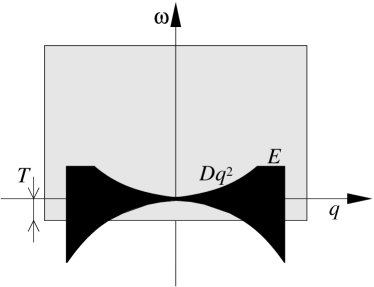
Figure 1: The $(q,\omega)$ plane. The power spectra in a metallic system are distributed pre-dominantly within the shaded rectangular area that indicates an implicit momentum cutoff (inverse of the mean free path), and an implicit high frequency absorption cutoff (related to the rate of collisions). For the SP-formula it is essential to realize that the spectral function $\tilde{S}^{\mbox{\tiny eq}}(q,\omega)$ of Eq.(53) has a lower emission cutoff which is determined by the temperature $T$. The power spectrum $\tilde{P}(-q,-\omega)$ of either Eq.(LABEL:e19) or Eq.(21), which is associated with the diffusive motion of a particle, is concentrated pre-dominantly within the dark region $|\omega|\lesssim Dq^{2}$. For the SP-formula it is essential to realize that the energy $E$ of the particle implies a frequency cutoff, which is analogous to $T$. Close to equilibrium one should take ${E\sim T}$.

It is important to discuss the significance of the many body result. To the extent that interactions can be neglected this result is exact and does not involve any uncontrolled semiclassical approximation. One realizes that

$$\tilde{P}^{[N]}(\omega)\ \ \approx\ \ \frac{1}{2}N_{T}\times{\tilde{P}}^{(0)}(\omega),\ \ \ \ \ \ \ \mbox{for $\omega{\ll}T$},$$ (16)

where $N_{T}=2T/\delta_{\mbox{\tiny F}}$ is the effective number of particles in the thermally smeared band around the Fermi surface. This factor is extensive, i.e. it grows linearly with the system’s volume. Only these particles can be excited by a small amount of energy $\omega\sim 0$ being absorbed from the environment, or, vice versa, they can release some energy into the environment. It is crucial to keep the physics of Pauli blocking correctly in this description. In fact, had we neglected the Pauli blocking, instead of Eq.(16) we would have obtained ${\tilde{P}^{[N]}(\omega)=N{\tilde{P}}^{(0)}(\omega)}$, where $N$ would have indicated the total number of particles in the system.

IV.3 The single excitation spectrum $P^{[1]}$

In the present subsection we would like to make contact with other descriptions in the literature, where the focus is on the dephasing of a single-particle excitation in the presence of a Fermi sea. Unlike the many-body calculation above, such point of view requires to introduce Pauli blocking factors ”by hand”. One finds (see Eq.(21) below) that the power spectrum of a thermalized one-particle excitation is

$$\tilde{P}^{[1]}(\omega)\ \ \approx\ \ \frac{1}{2}\times{\tilde{P}}^{(0)}(\omega),\ \ \ \ \ \ \ \mbox{for $\omega{\ll}T$},$$ (17)

which implies that Eq.(16) can be re-written as ${\tilde{P}^{[N]}(\omega)\approx N_{T}\tilde{P}^{[1]}(\omega)}$, which holds in the vicinity of the Fermi energy. One realizes that the factor $1/2$ reflects that Pauli blocking of the downward transitions and persists at high temperatures. The relation between the spectrum of the single-particle motion and the many-body density fluctuations is a central result of the present section. It will be employed in the next section to connect the one-body and the many-body dephasing rates.

In the spirit of the prevailing literature we consider separately electrons and holes of arbitrary energy, incorporating Pauli blocking factors “by hand” into the definition of the particle’s power spectrum. For an electron above the Fermi sea it has been claimed in Ref.[Cohen and Imry, 1999; Cohen, 1998] that the Fermi energy $E_{F}$ is like an effective potential floor. This is implied by the Fermi statistics, taking into account that a one-body-operator can change the state of only one electron. It also results from a more detailed analysis of the consequences of Pauli blocking on dephasing, which has been carried out both in the context of weak localization [Marquardt et al., 2007; von Delft et al., 2007] and ballistic interferometers [Marquardt, 2005, 2006], and which has been illustrated in exactly solvable models as well [Marquardt and Golubev, 2004; Marquardt and Golubev, 2005]. Consequently we define the power spectrum of an electron excitation with the appropriate Pauli blocking factors incorporated:

$$\tilde{P}^{[e]}(\omega;E) = \sum_{nm}(1{-}f(E_{m}))p_{n}|A_{mn}|^{2}\,2\pi\delta(\omega{-}(E_{m}{-}E_{n}))$$ (18)

$$= (1-f(E{+}\omega))\ {\tilde{P}}^{(0)}(\omega;E).$$

An analogous expression is introduced for holes:

$$\tilde{P}^{[h]}(\omega;E) = \sum_{nm}f(E_{m})p_{n}|A_{mn}|^{2}\,2\pi\delta(\omega{-}(E_{n}{-}E_{m}))$$ (19)

$$= f(E{-}\omega)\ {\tilde{P}}^{(0)}(\omega;E).$$

We can thermally average over $E$ using the prescription

$$\overline{G(E)}\ \ \equiv\ \ \int_{-\infty}^{\infty}G(E)\ [-f^{\prime}(E)]dE$$ (20)

where $f(E)$ is the Fermi occupation function which is determined by the Fermi energy $E_{\mbox{\tiny F}}$ and the temperature $T$. Then we get

$$\tilde{P}^{[1]}(\omega)\ \ \equiv \ \ \overline{\tilde{P}^{[e]}(\omega;E)}\ \ =\ \ \overline{\tilde{P}^{[h]}(\omega;E)}$$ (21)

$$= \ \ \frac{d}{d\omega}\left[\frac{\omega}{1-\mbox{e}^{-\omega/T}}\right]\times{\tilde{P}}^{(0)}(\omega;E_{\mbox{\tiny F}}).$$

Note that, at zero temperature, the first factor is just a step-function $\theta(\omega)$, cutting off the contributions from negative frequencies.

IV.4 Density fluctuations

By specializing the above general discussion to the case that $\hat{A}$ represents the density operator, and using the reasoning of the present section, we can define the $\tilde{P}^{[e]}(q,\omega;E)$ of an electron in the Fermi sea; the $\tilde{P}^{[h]}(q,\omega;E)$ of a hole in the Fermi sea; the $\tilde{P}^{[1]}(q,\omega)$ of a single particle excitation at equilibrium; and the $\tilde{P}^{[N]}(q,\omega)$ of the whole many body electronic system.

The results Eq.(21), Eq.(18), Eq.(19) and Eq.(LABEL:e19), as well as the approximations Eq.(17) and Eq.(16) for the power spectrum of the system are all of the form

$$\tilde{P}(q,\omega)\ \ =\ \ f_{p}(\omega)\,{\tilde{P}}^{(0)}(q,\omega).$$ (22)

where $f_{p}(\omega)$ reflects the way in which the Fermi occupation statistics manifests itself.

V Dephasing of a many-fermion system for weak coupling to the environment

The purpose of this section is to work out the many-body dephasing rate $\Gamma_{\varphi}^{[N]}$ according to SP-theory, and to compare it with the single-particle dephasing rate $\Gamma_{\varphi}^{[1]}$ that is obtained after incorporating Pauli blocking factors into the spectra, as described in the previous section. We will see they are equal, up to a factor describing the number of thermally excited particles that effectively can participate in the processes leading to dephasing.

Before we derive the dephasing rate, we set up a few simplifications in the notation. The integrand of the “SP formula” Eq.(9) includes a product of two spectral functions. We assume that the “bath” is in thermal equilibrium and therefore the detailed balance condition that should be satisfies is:

$$\frac{\tilde{S}(q,\omega)}{\tilde{S}(q,-\omega)}\ \ =\ \ \mbox{e}^{\omega/T}.$$ (23)

It follows that the spectral function can be written as

$$\tilde{S}(q,\omega)\ \ =\ \ \left[\frac{2\omega}{1-\mbox{e}^{-\omega/T}}\right]\,\eta(q,\omega),$$ (24)

where $\eta(q,\omega)$ is a symmetric function. It represents a generalized friction coefficient (in analogy to the standard notation in the Caldeira-Leggett model). Note that at high temperatures we have ${\tilde{S}(q,\omega)=2\eta T}$.

Without any approximation involved, because the $d\omega$ integration extends from $-\infty$ to $\infty$, the integrand of the “SP formula” can be symmetrized using the replacement

$$F(\omega)\ \ \mapsto\ \ \{F(\omega)\}_{\mbox{\tiny sym}}\equiv\frac{1}{2}[F(\omega)+F(-\omega)].$$ (25)

It is now natural to combine the prefactors in Eq.(24) and Eq.(22) into a “frequency-dependent temperature” for $\omega$ transitions:

$$T(\omega)\ \ \equiv\ \ \left\{\left[\frac{2\omega}{1-\mbox{e}^{-\omega/T}}\right]f_{p}(-\omega)\right\}_{\mbox{\tiny sym}}.$$ (26)

and to define an associated symmetrized spectral function for the effective thermal fluctuation of the environment:

$$\tilde{S}^{(0)}(q,\omega)\ \ \equiv\ \ 2\eta(q,\omega)T(\omega).$$ (27)

These definitions allow the “SP formula” to be written in a symmetrized form that involves a product of functions that are symmetric in $\omega$. Namely,

$$\Gamma_{\varphi}=\frac{1}{2}\int dq\int\frac{d\omega}{2\pi}\,\tilde{S}^{(0)}(q,\omega)\,{\tilde{P}}^{(0)}(q,\omega).$$ (28)

In the following subsections we shall discuss the functional form of $T(\omega)$ which is crucial for the calculation of low temperature dephasing. But first let us illuminate the outcome of Eq.(28) in what can be termed the semiclassical Nyquist limit. Namely, considering high temperatures, for which not only ${\tilde{P}}^{(0)}$ but also $\tilde{S}^{(0)}$ are classical-alike, one realizes that Eq.(28) still contains a non-classical $1/2$ due to the Pauli blocking of the downward transitions. So strictly speaking Eq.(28) does not possess a classical limit. If $\eta$ is independent of $\omega$ and the motion of the particle involves only small frequencies ${|\omega|\ll T}$, then $T^{[1]}(\omega)$ in the integrand of Eq.(28) can be replaced by the temperature $T$, and we get the simple result

$$\Gamma_{\varphi}^{[1]}\ \ =\ \ \alpha T,$$ (29)

where the dimensionless $\alpha$ is the $dq$ integral over $\eta$. But if we consider (say) a diffusive electron, then at low temperatures its power spectrum is broader than $T$ if ${q>(T/D)^{1/2}}$, as illustrated in Fig.1. Then the weight which is provided by $T(\omega)$ is like an effective cutoff, leading to non-linear dependence on the temperature. See e.g. [Cohen and Imry, 1999; Cohen, 1998] for a gallery of various results.

V.1 The dephasing rate of quasi particles at equilibrium

The calculation of the one body dephasing rate $\Gamma_{\varphi}^{[1]}$ involves the spectral function $\tilde{P}^{[1]}(q,\omega)$ of Eq.(21) and hence

$$T(\omega)^{[1]}\equiv\left\{\left[\frac{2\omega}{1-\mbox{e}^{-\omega/T}}\right]\frac{d}{d\omega}\left[\frac{\omega}{1-\mbox{e}^{\omega/T}}\right]\right\}_{sym}.$$ (30)

The calculation of the $N$ body dephasing rate $\Gamma_{\varphi}^{[N]}$ involves the spectral function $\tilde{P}^{[N]}(q,\omega)$ of Eq.(LABEL:e19) and hence

$$T(\omega)^{[N]}\equiv\left\{\left[\frac{2\omega}{1-\mbox{e}^{-\omega/T}}\right]\left[\frac{-\omega/\delta_{\mbox{\tiny F}}}{1-\mbox{e}^{\omega/T}}\right]\right\}_{sym}.$$ (31)

Doing the algebra we get

$$T(\omega)^{[1]}\ \ =\ \ \left[\frac{(\omega/2T)}{\sinh(\omega/2T)}\right]^{2}\,T,$$ (32)

and $T(\omega)^{[N]}=(2T/\delta_{\mbox{\tiny F}})T(\omega)^{[1]}$, leading to

$$\Gamma_{\varphi}^{[N]}\ \ =\ \ \left(2\frac{T}{\delta_{\mbox{\tiny F}}}\right)\Gamma_{\varphi}^{[1]}.$$ (33)

We have thus come to the conclusion that the many-body dephasing rate $\Gamma_{\varphi}^{[N]}$ is equal to the single-excitation dephasing rate $\Gamma_{\varphi}^{[1]}$ which properly incorporates Pauli blocking, multiplied by a factor $N_{T}=2T/\delta_{\mbox{\tiny F}}$ that counts the number of thermally excited particles. At this point it is important to emphasize that if the interfering entity (system) consists of $N_{s}$ constituent particles, all interacting in the same way with the environment, one expects the dephasing rate to be $N_{s}$ times the dephasing rate for a single constituent particle under the same conditions. This is why larger systems are expected to decohere faster [Ze1, ; Ze2, ]. In our case the effective number of participating particles in the system is $N_{T}$ irrespective of the actual total number. Thus, without putting in ”by hand” any Pauli blocking factors, we have re-derived the correct result that is obtained from a more sophisticated diagrammatic or path-integral analysis [Marquardt et al., 2007; von Delft et al., 2007]. It is therefore possible to regard $\Gamma_{\varphi}^{[1]}$ as the dephasing rate per effective particle. Equation (33) represents a central result of the present paper, whose consequences and modifications will be discussed in the following.

V.2 The dephasing rate of a non-equilibrium excitation

It is interesting as well to consider the dephasing rate for a non-equilibrium one-particle excitation at some energy $E$. Then we cannot simply start from the many-body spectrum $\tilde{P}^{[N]}$ which is calculated for the thermal equilibrium state of the many-body problem. To make contact with previous approaches in the literature [Marquardt et al., 2007], we briefly formulate the nonequilibrium dephasing rate in terms of the present notations. In Ref.[Marquardt et al., 2007] it has been argued that the dephasing rate should be calculated as

$$\Gamma_{\varphi}^{\mbox{\tiny noneq}}(E)=\frac{1}{2}\left(\Gamma_{\varphi}^{[e]}(E)+\Gamma_{\varphi}^{[h]}(E)\right).$$ (34)

If we make a thermal average over $E$ both terms are equal, but if we consider non-equilibrium excitations a more careful treatment is required. Using the expressions for ${\tilde{P}^{[e]}(q,\omega;E)}$ and ${\tilde{P}^{[h]}(q,\omega;E)}$, the corresponding function in Eq.(22) is

$$f_{p}(\omega)=[1-f(E{+}\omega)+f(E{-}\omega)]/2,$$ (35)

hence

$$T(\omega)=\left\{\left[\frac{\omega}{1{-}\mbox{e}^{-\omega/T}}\right]\Big{(}1{-}f(E{-}\omega){+}f(E{+}\omega)\Big{)}\right\}_{sym}.$$ (36)

Doing the algebra we get

$$T(\omega)=\left[\left(\frac{1}{\mbox{e}^{\omega/T}{-}1}\right)+\frac{1}{2}\Big{(}1{-}f(E{-}\omega)+f(E{+}\omega)\Big{)}\right]\omega$$

$$=\left[\coth\left(\frac{\omega}{2T}\right)+\frac{1}{2}\tanh\left(\frac{E{-}\omega}{2T}\right)-\frac{1}{2}\tanh\left(\frac{E{+}\omega}{2T}\right)\right]\omega,$$

which agrees with Ref.[Marquardt et al., 2007].

VI Dephasing of electrons with screening: The diagrammatic perspective

Up to now, we have treated the weak-coupling case, in which neither the particle dynamics (i.e. the density fluctuations) nor the potential fluctuations are influenced appreciably by the presence of interactions. It is for this reason that we have been able to derive the total particle decay rate in such a simple manner, expressing it through the product of correlators $\tilde{P}$ and $\tilde{S}$, associated with the particle dynamics and the potential fluctuations, respectively.

More care has to be exercised when one tries to extend the framework to cases in which the potential fluctuations themselves change strongly (even qualitatively) after switching on the interaction. The most important example concerns the effect of the long-range Coulomb interaction in a metal. The long-range repulsion suppresses efficiently long-wavelength, low-frequency density fluctuations and the associated potential fluctuations, thus giving rise to screening. An important counter-intuitive (yet well-known) consequence is that the potential spectrum at small $\omega,q$ is independent of the electron charge (see Eq.(53)).

It will turn out that, for such a situation, the single-particle decay rate is not correctly reproduced with a naive ansatz, in which both $\tilde{S}$ and $\tilde{P}$ are obtained for the full interacting system (neither, of course, can we neglect interactions completely in both $\tilde{S}$ and $\tilde{P}$). To shed light on this issue, we now rephrase the results of the “SP theory” developed here in terms of diagrams.

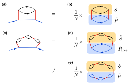
Figure 2: The relation between “SP theory” and standard diagrammatics: (a) Diagrammatic calculation of the single-particle decay rate to leading order in the density-density interaction. (b) When applying the “SP theory” to a many-body system, one effectively calculates an extensive diagram, whose value scales with the number of affected particles (here denoted as “$N$”). (c) For a metal with screening, diagrams of this type have to be summed to yield the single-particle decay rate in RPA. (d) After translation into the diagrams appearing in the “SP theory”, we see that the bare particle-hole bubble has to be used in describing the system’s motion, in contrast to (e).

VI.1 Diagrams for the weak-coupling limit

We first return to the weak-coupling case. In that limit, the single-particle decay rate is obtained in a diagram of the type shown in Fig.2(a). It represents the interaction of the given particle with the density-fluctuations described by the bubble. Turning to SP-theory, we see the following: Its straightforward application to a many-body system produces a diagram of the type shown in Fig.2(b). This diagram has no external lines, and is therefore extensive, i.e. its value grows with volume. More precisely, as elaborated in our previous discussion, it yields the decay rate multiplied by the number of particles that can be scattered. Once this feature is taken into account, one can deduce the single-particle decay rate.

VI.2 Diagrams beyond weak-coupling

Let us now have a look at the strong-coupling case, where screening alters drastically the fluctuations of the density and the potential. Within the random phase approximation (RPA), the single-particle decay rate can be calculated using diagrams of the type shown in Fig.2(c), with an arbitrary number of polarization bubbles inserted to account for screening. In this way, the correct modified fluctuation spectrum $\tilde{S}$ enters the decay rate. When translating this into an appropriate extensive diagram (Fig.2(d)), the open-ended single-particle line turns into one particle-hole bubble. The latter corresponds to the density-density correlator evaluated in the absence of interactions. In contrast, in a literal (naive) application of SP-theory to the many-body problem with screening one might be tempted to employ the screened density-density propagator (Fig.2(e)), which gives incorrect results.

The source of the difficulty is quite obvious when comparing Fig. 2(e) to Fig. 2(c): The origin of the bubble is the single-particle line, which appears since we are interested in the coherent propagation of the particle. We are not interested in the propagation of a density perturbation that enters diagram (e).

The issue discussed here is independent of whether we are in the ballistic or the diffusive regime, or of what are the details of the model. In any case, the correct application of the SP-theory requires to employ the full potential fluctuations (including screening) for $\tilde{S}$, while looking at the bare $\tilde{P}_{{\mbox{\tiny free}}}^{[N]}$, calculated for the non-interacting system.

VII Self consistent point of view for the dephasing of interacting electrons

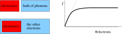
Figure 3: We first consider non-interacting electrons in a boxrmA of volume $L^{d}$ coupled to a bath of phonons at temperature $T$. The solid curve on the right illustrates how the decay rate of the purity depends on the number of electrons in the system. If the electrons were not identical (dotted line) one would get ${\Gamma=N\Gamma^{[1]}}$, but due to the Fermi statistics one obtains a saturation at ${\Gamma=N_{T}\Gamma^{[1]}}$. In the case of $N$ interacting electrons in a dirty metal, with no bath of phonons involved, one can define a bunch of $N_{s}$ test particles as the systemrmB , while all the other $N{-}N_{s}$ electrons constitute the fluctuating environment. We have in mind ${N_{s}\ll N}$, while for ${(N{-}N_{s})\ll N}$, the role of system and environment is flipped.

We now want to clarify within the SP approach how screening should be handled, and demonstrate the consistency with the diagrammatic perspective of Section VII. In a dirty metal the motion of electrons is diffusive, and there is a screening effect due to the long range Coulomb interaction. The fluctuations of the electrostatic potential $U$ reflect the many-body fluctuations in the density of the electrons via the Coulomb law

$$\tilde{S}(q,\omega)\ \ =\ \ \frac{1}{L^{d}}\left(\frac{4\pi e^{2}}{q^{2}}\right)^{2}\ \tilde{P}(q,\omega),$$ (37)

with $\tilde{S}$ and $\tilde{P}$ defined by Eqs. (7) and (8) respectively. The equilibrium fluctuations of the induced electrostatic fluctuations $\tilde{S}^{\mbox{\tiny eq}}(q,\omega)$ are trivially related to the dynamic form factor $\tilde{P}^{\mbox{\tiny eq}}(q,\omega)$ by the above relation, and can be determined self consistently using the fluctuation-dissipation relation (see App.C):

$$\tilde{S}^{\mbox{\tiny eq}}(q,\omega)\ \ =\ \ \frac{1}{\nu Dq^{2}}\left[\frac{2\omega}{1-\mbox{e}^{-\omega/T}}\right].$$ (38)

If we want to calculate the single-particle dephasing rate $\Gamma_{\varphi}^{[1]}$, then one option is to obtain $\tilde{P}^{[1]}(q,\omega)$ from a blend of semiclassical and many-body considerations as in Section IV. But we are trying in this paper to explore an alternative route, where the single particle dephasing rate is defined as the many-body dephasing rate $\Gamma_{\varphi}^{[N]}$ per effective particle as in Eq.(33). The main difficulty that immediately arises, once interacting electrons are concerned, is how to define the “system” for which the calculation is done. The proper formulation of the system-bath paradigm becomes tricky once electrons are both the “system” and the “bath” (see illustration in Fig.3). In particular we have to determine what is $\tilde{P}^{[N]}(q,\omega)$ for the case that screening is important. Here we encounter a conflict between two opposing points of view, which we discuss below.

There are two ways to determine $\tilde{P}^{[N]}(q,\omega)$. On the one hand, within the framework of the heuristic semiclassical approach of Section IV, the spectral function $\tilde{P}^{[N]}(q,\omega)$ should be given by Eq.(LABEL:e19) which treats the electrons as non-interacting. On the other hand, within the formal framework it describes the fluctuations of the many body density of the electrons, and therefore should equal $\tilde{P}^{\mbox{\tiny eq}}(q,\omega)$ as defined after Eq.(37). But then one realizes that for an interacting system $\tilde{P}^{[N]}(q,\omega)$ is very different from $\tilde{P}^{\mbox{\tiny eq}}(q,\omega)$. So it seems that we have here an inconsistency.

In order to resolve the apparent inconsistency we have to clarify the physical meaning of the phrase “dephasing rate per particle”. This notion is not problematic conceptually if the environment is a distinct entity (phonon bath). But in the case of a dirty metal this distinction is blurred: obviously we cannot regard the same particles as both the “system” and “environment”.

It turns out that a reconciliation of the formal fluctuation-dissipation analysis with the heuristic approach is possible provided we define the “system” as a bunch of non-interacting test particlesrmC , whose density fluctuations are simply those of diffusing, non-interacting electrons. We can obtain the power-spectrum of the ‘minority’ test particles, starting from Eq.(47), but replacing $U_{\mbox{\tiny total}}$ by the fluctuating potential $\mathcal{U}$ produced by the ’majority’ particles. This effectively omits screening effects in the calculation of the test particle density fluctuations:

$$\rho_{q,\omega}\ \ =\ \ \frac{(\sigma/e^{2})q^{2}}{i\omega-Dq^{2}}\ \mathcal{U}_{q,\omega}.$$ (39)

Note that the $\rho$ of the system (minority fraction of electrons) is assumed to be much smaller than the total electronic density $\rho_{\mbox{\tiny elct}}$ that appears in the FDT derivation, hence one can neglect the back-reaction effect. In other words, as far as the minority $\rho$ is concerned we do not take the screening into account, and treat them as non-interacting. From Eq.(39), together with Eqs.(7) and (8) and the Einstein relation $\sigma=e^{2}D\nu$, we get immediately

$$\tilde{P}^{[N]}(q,\omega)\ \ = \ \ L^{d}\,\left|\frac{\nu Dq^{2}}{i\omega-Dq^{2}}\right|^{2}\ \tilde{S}^{\mbox{\tiny eq}}(q,\omega)$$ (40)

$$= \ \ \frac{\omega/\delta_{\mbox{\tiny F}}}{1-\mbox{e}^{-\omega/T}}\ {\tilde{P}}^{(0)}(\omega;E_{\mbox{\tiny F}}),$$ (41)

where for the second line we recalled Eq. (14) for ${\tilde{P}}^{(0)}$ and Eq. (53) for $\tilde{S}^{\mbox{\tiny eq}}$. This result agrees with Eq.(LABEL:e19) as if we could regard the electrons as diffusing but non-interacting. It is important to appreciate that we have obtained here a non-trivial profound relation that bypasses the heuristic approach which is required in order to adopt Eq.(LABEL:e19) for strongly interacting electrons: strictly speaking the derivation that leads to Eq.(LABEL:e19) is not applicable here. Still we get Eq.(40) which agrees with Eq.(LABEL:e19) by extending the common fluctuation-dissipation reasoning, without the need to introduce a blend of semiclassics with Pauli exclusion factors.

VIII Conclusions

We have presented a straightforward approach to the calculation of the dephasing rate within the framework of Fermi golden rule picture, and applied it to a many-fermion system. Starting from the quantum spectra of the environment ($\tilde{S}$) and the system ($\tilde{P}$), the approach (termed here ”SP-theory”) yields the dephasing rate as an integral over the frequency transferred between system and environment during interaction processes. In the present paper, we have gone beyond previous attempts, and considered a full many-fermion system. We have argued that this yields results which automatically incorporate the crucial physics of Pauli blocking that serves to suppress decoherence at low temperatures. The many-body dephasing rate can be identified as the single-particle dephasing rate times the effective number of thermally excited particles susceptible to scattering. The use of non-symmetrized spectral functions provides in a natural way the proper cutoff scheme for the frequency integral of the ”SP formula”, without having to invoke the ad hoc cutoff schemes that had been introduced in previous publications.

By defining the single particle dephasing as the many-body dephasing per particle one can bypass the need to use a blend of semiclassics with Pauli exclusion factors. This point of view also provides a natural bridge to the diagrammatic approach. Indeed we have shown how the results of the SP-theory can be interpreted in terms of diagrams. This has allowed us to address another question, namely how SP-theory should be applied in a situation in which the system-environment coupling is no longer weak. That is the situation relevant for electrons moving in a disordered metal, where screening is crucial for the structure of the Nyquist noise. We have shown that SP-theory should incorporate in such a case the full environment spectrum, alongside the non-interacting density spectrum of the system, in agreement with the diagrammatic approach.

Acknowledgment: We thank Ora Entin-Wohlman and Baruch Horovitz for useful discussions. The research has been supported by a grant from the DIP, the Deutsch-Israelische Projektkooperation (contract H-2-1), as well as by the DFG through the Emmy-Noether program (FM) and SFB TR 12. This research was supported in part by the National Science Foundation under Grant No. NSF PHY05-51164, and by the USA-Israel Binational Science Foundation (BSF).

Appendix A The semiclassical picture of dephasing

The notion of dephasing naturally arises in the analysis of transport where, loosely speaking, one is interested in calculating the probability of a particle to get from one point to a different point. Consequently the most popular definition of the dephasing factor is based on a semiclassical picture. Using the Feynman-Vernon formalism, and adopting the notations as in Ref.[Cohen and Imry, 1999; Cohen, 1998], the propagator of the reduced probability matrix in the presence of a thermal bath, is expressed as a sum over pairs of classical trajectories:

$$\sum_{ab}A_{a}A_{b}^{*}\exp\left(-\frac{S_{N}[x_{a},x_{b}]}{\hbar^{2}}\right)\ \exp\left(i\frac{S[x_{a}]{-}S[x_{b}]}{\hbar}\right).$$ (42)

The dephasing factor $P_{\varphi}(t)$ is defined as a number within $[0,1]$ that characterizes the suppression of the off-diagonal elements: One observes that after time $t$ the interference contribution, that comes from the off diagonal terms in the double sum, is suppressed by a factor

$$P_{\varphi}(t)=\mbox{e}^{-S_{N}[x^{A},x^{B}]}\equiv\Big{|}\ \Big{\langle}\ U[x_{a}]\chi\ \Big{|}\ U[x_{b}]\chi\ \Big{\rangle}\ \Big{|},$$ (43)

where $\chi$ is the preparation of the bath. In order not to complicate the notations, the canonical average over the $\chi$ states is implicit. The unitary operator $U[x]$ generates the evolution of the bath given that the particle goes along the trajectory $x(t)$. The action $S_{N}[x_{a},x_{b}]$ is a double time integral. Using manipulation as in Refs. [Cohen and Imry, 1999; Cohen, 1998] one obtains the “SP formula” with the symmetrized version of $\tilde{S}(q,\omega)$, and the symmetric classical version of $\tilde{P}(q,\omega)$, namely ${\tilde{P}}^{(0)}$ of Eq.(14).

The semiclassical expression is definitely wrong for short range scattering at low temperatures [Cohen and Imry, 1999; Cohen, 1998], because it does not reflect that closed channels cannot be excited. This problem with the semiclassical (stationary phase) approximation is well known in the theory of inelastic scattering.

Appendix B The purity based definition of dephasing

The following appendix follows the presentation of Ref. [Cohen and Horovitz, 2007, 2008]. The natural definition for the dephasing factor $P_{\varphi}(t)$ is related to the purity $\mbox{trace}(\rho^{2})$ of the reduced probability matrix. Given that the state of the system including the environment is $\Psi_{pn}$, where $p$ and $n$ label the basis states of the particle and the bath respectively, the full probability matrix is $\Psi_{pn}\Psi_{p^{\prime}n^{\prime}}^{*}$, while the purity of the reduce probability matrix is

$$P_{\varphi}(t) = \sqrt{\mbox{trace}(\rho_{\mbox{\tiny sys}}^{2})}=\sqrt{\mbox{trace}(\rho_{\mbox{\tiny env}}^{2})}$$ (44)

$$= \left[\sum_{p^{\prime}p^{\prime\prime}n^{\prime}n^{\prime\prime}}\Psi_{p^{\prime}n^{\prime}}\Psi_{p^{\prime\prime}n^{\prime}}^{*}\Psi_{p^{\prime\prime}n^{\prime\prime}}\Psi_{p^{\prime}n^{\prime\prime}}^{*}\right]^{1/2}.$$

Assuming a factorized initial preparation as in the conventional Feynman-Vernon formalism, we propose the rate of loss of purity as a measure for decoherence. A standard reservation applies: initial transients during which the system gets “dressed” by the environment should be ignored as these reflect renormalizations due to the interactions with the high frequency modes. Other choices of initial state might involve different transients, while the later slow approach to equilibrium should be independent of these transients. In any case the reasoning here is not much different from the usual ideology of the Fermi golden rule, which is used with similar restrictions to calculate transition rates between levels.

Writing the initial preparation as ${\Psi^{(0)}_{pn}=\delta_{p,p_{0}}\delta_{n,n_{0}}}$, and using leading order perturbation theory, we can relate $P_{\varphi}$ to the probabilities ${P_{t}(p,n|p_{0},n_{0})=|\Psi_{pn}|^{2}}$ to have a transition from the state $|p_{0},n_{0}\rangle$ to the state $|p,n\rangle$ after time $t$. The derivation is detailed in Appendix E of Ref.[Cohen and Horovitz, 2007, 2008]. One obtains the result

$$P_{\varphi}(t) = P_{t}(p_{0},n_{0}|p_{0},n_{0})$$

$$+ P_{t}(p{\neq}p_{0},n_{0}|p_{0},n_{0})+P_{t}(p_{0},n{\neq}n_{0}|p_{0},n_{0}).$$

The notation $p\neq p_{0}$ or $n\neq n_{0}$ implies a summation $\sum_{p\neq p_{0}}$ or $\sum_{n\neq n_{0}}$, respectively. The actual calculation of $P_{t}(p,n|p_{0},n_{0})$ can be done using Fermi’s golden rule (FGR) as discussed in the main text.

Thus we see that within the FGR framework, the purity is simply the probability that either the system or the bath do not make a transition. Accordingly $P_{\varphi}(t)$ is essentially the same as the survival probability $P(t)$ of the initial state (the first term in Eq.(B)). In typical circumstances the difference between $P_{\varphi}(t)$ and $P(t)$ has zero measure weight in the $dqd\omega$ integration and therefore $\Gamma_{\varphi}$ can be identified with the Wigner decay rate of system excitations.

Appendix C The fluctuation-dissipation relation

The dielectric constant of a metal is defined via the linear relation between the total electrostatic potential $U_{\mbox{\tiny total}}$ and an external test charge density $\rho_{\mbox{\tiny ext}}$

$$U_{\mbox{\tiny total}}\ \ =\ \ \frac{1}{\varepsilon(q,\omega)}\left(\frac{4\pi e^{2}}{q^{2}}\right)\rho_{\mbox{\tiny ext}}.$$ (46)

For simplicity we relate here and below to one component $q$ of the fields. The total electrostatic potential is the sum of the external potential $U_{\mbox{\tiny ext}}=(4\pi e^{2}/q^{2})\rho_{\mbox{\tiny ext}}$, and the induced potential $U=(4\pi e^{2}/q^{2})\rho_{\mbox{\tiny elct}}$, where $\rho_{\mbox{\tiny elct}}$ is the total density of the electrons. The dielectric constant can be deduced from the equations of motion ${\partial\rho_{\mbox{\tiny elct}}/\partial t=-\nabla J}$ with ${J=-(\sigma/e^{2})\nabla U_{\mbox{\tiny total}}-D\nabla\rho_{\mbox{\tiny elct}}}$ that leads to the relation

$$\rho_{\mbox{\tiny elct}}\ \ =\ \ \frac{(\sigma/e^{2})q^{2}}{i\omega-Dq^{2}}\ U_{\mbox{\tiny total}},$$ (47)

and hence to ${U_{\mbox{\tiny total}}=(1/\varepsilon)U_{\mbox{\tiny ext}}}$, where

$$\varepsilon(q,\omega)=1-\frac{4\pi\sigma}{i\omega-Dq^{2}}.$$ (48)

Note that

$$\mbox{Im}\left[\frac{-1}{\varepsilon(q,\omega)}\right]=\frac{4\pi\sigma\omega}{(Dq^{2}+4\pi\sigma)^{2}+\omega^{2}}\approx\frac{\omega}{4\pi\sigma}.$$ (49)

The interaction between the electrons and an external electrostatic field is described by ${\mathcal{H}_{\mbox{\tiny ext}}=U_{\mbox{\tiny ext}}\rho_{\mbox{\tiny elct}}}$ which can be also written as ${\mathcal{H}_{\mbox{\tiny ext}}=\rho_{\mbox{\tiny ext}}U}$. The fluctuation dissipation relation expresses $\tilde{S}^{\mbox{\tiny eq}}(q,\omega)$ using the response function $\alpha(q,\omega)$ that relates $U$ to $-\rho_{\mbox{\tiny ext}}$ which is

$$\alpha(q,\omega)=\frac{4\pi e^{2}}{q^{2}}\left[1-\frac{1}{\varepsilon(q,\omega)}\right].$$ (50)

Namely,

$$\tilde{S}^{\mbox{\tiny eq}}(q,\omega)=\mbox{Im}\Big{[}\alpha(q,\omega)\Big{]}\,\left(\frac{2}{1-\mbox{e}^{-\omega/T}}\right),$$ (51)

leading to

$$\tilde{S}^{\mbox{\tiny eq}}(q,\omega)\approx\frac{e^{2}}{\sigma}\frac{1}{q^{2}}\left(\frac{2\omega}{1-\mbox{e}^{-\omega/T}}\right).$$ (52)

The Ohmic behavior is cut-off by $|\omega|\lesssim 1/\tau_{c}$ and $|q|\lesssim{1}/{\ell}$ where $\ell=v_{\mbox{\tiny F}}\tau_{c}$ is the elastic mean free path, and $v_{\mbox{\tiny F}}$ is the Fermi velocity. Recalling the Einstein relation ${\sigma=e^{2}\nu D}$, where $\nu=\delta_{\mbox{\tiny F}}^{-1}/L^{d}$ is the density of states per unit volume, we can write this result more conveniently as follows:

$$\tilde{S}^{\mbox{\tiny eq}}(q,\omega)\approx\frac{1}{\nu Dq^{2}}\left(\frac{2\omega}{1-\mbox{e}^{-\omega/T}}\right).$$ (53)

Note that the electron charge $e$ cancels out from this final result for the Nyquist noise spectrum. This well-known fact is due to the effects of screening: A larger value of the charge would be canceled by a correspondingly stronger suppression of density fluctuations.

References

- (1)
- Altshuler et al. (1982) B. Altshuler, A. Aronov, and D. Khmelnitskii, J. Phys. C 15, 7367 (1982).
- Fukuyama and Abrahams (1983) H. Fukuyama and E. Abrahams, Phys. Rev. B 27, 5976 (1983).
- Aleiner et al. (1999a) I. L. Aleiner, B. L. Altshuler, and M. E. Gershenson, Waves in Random Media 9, 201 (1999a).
- Aleiner et al. (1999b) I. L. Aleiner, B. L. Altshuler, and M. E. Gershenson, Phys. Rev. Lett. 82, 3190 (1999b).
- Aleiner et al. (2002) I. Aleiner, B. Altshuler, and M. Vavilov, arXiv:cond-mat/0208264 (2002).
- von Delft et al. (2007) J. von Delft, F. Marquardt, R. A. Smith, and V. Ambegaokar, Phys. Rev. B 76, 195332 (2007).
- Cohen (1998) D. Cohen, J. Phys. A 31, 8199 (1998).
- Cohen and Imry (1999) D. Cohen and Y. Imry, Phys. Rev. B 59, 11143 (1999).
- Imry (2002) Y. Imry, Introduction to Mesoscopic Physics (Oxford University Press, 2002), second edition ed.
- Marquardt et al. (2007) F. Marquardt, J. von Delft, R. A. Smith, and V. Ambegaokar, Phys. Rev. B 76, 195331 (2007).
- Stern et al. (1990) A. Stern, Y. Aharonov, and Y. Imry, Phys. Rev. A 41, 3436 (1990).
- Cohen and Horovitz (2007) D. Cohen and B. Horovitz, J. Phys. A 40, 12281 (2007).
- Cohen and Horovitz (2008) D. Cohen and B. Horovitz, Europhysics Letters 81, 30001 (2008).
- Chakravarty and Schmid (1986) S. Chakravarty and A. Schmid, Phys. Rep. 140, 193 (1986).
- Golubev and Zaikin (1998) D. S. Golubev and A. D. Zaikin, Phys. Rev. Lett. 81, 1074 (1998).
- Golubev and Zaikin (1999) D. S. Golubev and A. D. Zaikin, Phys. Rev. B 59, 9195 (1999).
- von Delft (2008) J. von Delft, International Journal of Modern Physics B 22, 727 (2008), arXiv:cond-mat/0510563.
- (19) G.B. Lesovik and R. Loosen, JETP Lett. 65, 269 (1997).
- (20) U. Gavish, Y. Levinson, and Y. Imry, Phys. Rev. B 62, R10637 (2000).
- Clerk et al. (accepted, 2009) A. A. Clerk, M. H. Devoret, S. M. Girvin, F. Marquardt, and R. J. Schoelkopf, arXiv:0810.4729, Reviews of Modern Physics (accepted, 2009).
- (22) U. Weiss, Quantum Dissipative Systems (World Scientific, Singapore, 1999).
- Marquardt (2005) F. Marquardt, Europhysics Letters 72, 788 (2005).
- Marquardt (2006) F. Marquardt, Phys. Rev. B 74, 125319 (2006).
- Marquardt and Golubev (2004) F. Marquardt and D. S. Golubev, Phys. Rev. Lett. 93, 130404 (2004).
- Marquardt and Golubev (2005) F. Marquardt and D. S. Golubev, Phys. Rev. A 72, 022113 (2005).
- (27) O. Nairz, M. Arndt and A. Zeilinger, American Journal of Physics 71, 319 (2003).
-
(28)
B. Brezger, L. Hackermüller, S. Uttenthaler, J. Petschinka, M. Arndt, and A. Zeilinger,
Phys. Rev. Lett. 88, 100404 (2002).
- (29) For the purpose of this illustration we assume that the velocity and hence the diffusion coefficient of the electron do not depend on its kinetic energy (a linear dispersion relation). The electrons are added one by one, and at low densities form a Boltzmann gas. Only when the chemical potential exceeds one starts to observe the implications of Fermi statistics.
- (30) To label one or several electrons as test particles is of course meaningless if we take their indistinguishablity into account. So the dashed line has some meaning only in a vague semiclassical context which we try to bypass. If we literally divided the electron into two sub-volumes, the purity loss and hence the many-body dephasing rate would be proportional to the area of dividing surface that separate the two spatial regions.
- (31) The notion of “test particles” acquires a more concrete meaning within the context of a transport experiment, where the “test particles” are the ones contributing to the current, or even more to the point, in the context to weak localization, to the back-scattered current.