Temperature dependence of magnetic susceptibility of nuclear matter: lowest order constrained variational calculations

Abstract

In this paper we study the magnetic susceptibility and other thermodynamic properties of the polarized nuclear matter at finite temperature using the lowest order constrained variational (LOCV) method employing the $AV_{18}$ potential. Our results show a monotonic behavior for the magnetic susceptibility which indicates that the spontaneous transition to the ferromagnetic phase does not occur for this system.

I INTRODUCTION

The magnetic susceptibility is one of the most important magnetic properties of the dense matter, its behavior specifies whether the spontaneous phase transition to a ferromagnetic state occurs. This transition in nuclear matter could have important consequences for the physical origin of the magnetic field of the pulsars which are believed to be rapidly rotating neutron stars with strong surface magnetic fields in the range of $10^{12}-10^{13}$ Gauss shap ; paci ; gold ; navarro . Considering different stages of the neutron star formation at different temperatures, the study of the magnetic properties of the polarized nuclear matter at finite temperature is of special interest in the description of protoneutron stars. A protoneutron star (newborn neutron star) is born within a short time after the supernovae collapse. In this stage the interior temperature of the neutron star matter is of the order 20-50 MeV burro . The magnetic susceptibility of nucleonic matter is also an useful quantity to estimate the mean free path of the neutrino in the dense nucleonic matter which is relevant information for the understanding of the mechanism underlying the supernova explosion and the cooling process of the neutron stars iwamoto .

There exists several possibilities of the generation of the magnetic field in a neutron star. From the nuclear physics point of view, such a possibility has been studied by several authors using different theoretical approaches [7-30], but the results are still contradictory. In most calculations, the neutron star matter is approximated by pure neutron matter at zero temperature. The properties of the polarized neutron matter both at finite and zero temperature have been studied by several authors apv ; dapv ; bprrv . Some calculations show that the neutron matter becomes ferromagnetic for some densities brown ; rice ; pandh ; marcos ; apv . Some others, using the modern two-body and three-body realistic interactions, show no indication of the ferromagnetic transition at any density for the neutron matter and the asymmetrical nuclear matter kutsb ; fanto ; vida ; bprrv . The results of another calculation show both behaviors; the D1P force exhibits a ferromagnetic transition whereas no sign of such transition is found for D1 at any density and temperature dapv . The influence of the finite temperature on the antiferromagnetic (AFM) spin ordering in the symmetric nuclear matter with the effective Gogny interaction within the framework of a Fermi liquid formalism has been studied by Isayev isay1 ; isay2 . We note that in the symmetric nuclear matter corresponding to AFM spin ordering, we have $\Delta\rho_{\uparrow\downarrow}=(\rho_{n\uparrow}+\rho_{p\downarrow})-(\rho_{n\downarrow}+\rho_{p\uparrow})\neq 0$ and $\Delta\rho_{\uparrow\uparrow}=\rho_{\uparrow}-\rho_{\downarrow}=0$. In this article, we use the lowest order constrained variational (LOCV) formalism to investigate the possibility of the transition to a ferromagnetic phase for the polarized hot symmetrical nuclear matter.

The LOCV method has been developed to study the bulk properties of the quantal fluids OBI1 ; OBI2 ; OBI3 . This technique has been used for studying the ground state properties of finite nuclei and treatment of isobars BHIM ; MI1 ; MI2 . Modarres has extended the LOCV method to the finite temperature calculations and has applied it to the neutron matter, nuclear matter and asymmetrical nuclear matter in order to calculate the different thermodynamic properties of these systems Mod93 ; Mod95 ; Mod97 ; MM98 . Few years ago, we calculated the properties of nuclear matter at zero and finite temperature using the LOCV method with the new nucleon-nucleon potentials BM97 ; BM98 ; MB98 . The LOCV method has several advantages with respect to the other many-body formalism. These are as follows: (i) Since the method is fully self-consistent, it does not introduce any free parameters into the calculations. (ii) It considers the constraint in the form of a normalization constraint Feen to keep the higher-order terms as small as possible OBI3 ; MI1 ; MI2 ; MM98 ; BM97 and it also assumes a particular form for the long-range behavior of the correlation function in order to perform an exact functional minimization of the two-body energy with respect to the short-range behavior of the correlation function. (iii) The functional minimization procedure represents an enormous computational simplification over the unconstrained methods (i.e. to parameterize the short-range behavior of the correlation functions) which attempt to go beyond the lowest order.

Recently, we have computed the properties of the polarized neutron matter bordbig , polarized symmetrical bordbig2 and asymmetrical nuclear matters bordbig3 and also polarized neutron star matter bordbig3 at zero temperature using the microscopic calculations employing the LOCV method with the realistic nucleon-nucleon potentials. We have concluded that the spontaneous phase transition to a ferromagnetic state in these matters does not occur. We have also calculated the thermodynamic properties of the polarized neutron matter at finite temperature bordbig4 such as the total energy, magnetic susceptibility, entropy and pressure using the LOCV method employing the $AV_{18}$ potential wiring . Our calculations do not show any transition to a ferromagnetic phase for a hot neutron matter.

In the present work, we intend to apply the LOCV calculation for the polarized symmetrical nuclear matter at finite temperature using the $AV_{18}$ potential.

II Finite temperature calculations for polarized nuclear matter with the LOCV method

We consider a system of $A$ interacting nucleons with $A^{(+)}$ spin-up and $A^{(-)}$ spin-down nucleons. For this system, the total number density ($\rho$) and spin asymmetry parameter ($\delta$) are defined as

$$\rho = \rho^{(+)}+\rho^{(-)},$$

$$\delta = \frac{\rho^{(+)}-\rho^{(-)}}{\rho}.$$ (1)

$\delta$ shows the spin ordering of the matter which can have a value in the range of $\delta=0.0$ (unpolarized matter) to $\delta=1.0$ (fully polarized matter). To obtain the macroscopic properties of this system, we should calculate the total free energy per nucleon, $F$,

$$F=E-{\cal T}S^{(+)}-{\cal T}S^{(-)}.$$ (2)

$E$ is total energy per nucleon and $S^{(i)}$ is the entropy per nucleon corresponding to spin projection $i$,

$$S^{(i)}(\rho,T) = -\frac{1}{A}\sum_{k}\{[1-n^{(i)}(k,{\cal T},\rho^{(i)})]\textrm{ln}[1-n^{(i)}(k,{\cal T},\rho^{(i)})]$$ (3)

$$+n^{(i)}(k,{\cal T},\rho^{(i)})\textrm{ln}n^{(i)}(k,{\cal T},\rho^{(i)})\}.$$

where $n^{(i)}(k,{\cal T},\rho^{(i)})$ is the Fermi-Dirac distribution function,

$$n^{(i)}(k,{\cal T},\rho^{(i)})=\frac{1}{e^{\beta[\epsilon^{(i)}(k,{\cal T},\rho^{(i)})-\mu^{(i)}({\cal T},\rho^{(i)})]}+1}\cdot$$ (4)

In the above equation $\beta=\frac{1}{k_{B}{\cal T}}$ , $\mu^{(i)}$ being the chemical potential which is determined at any adopted value of the temperature $\cal T$, number density $\rho^{(i)}$ and spin polarization $\delta$, by applying the following constraint,

$$\sum_{k}n^{(i)}(k,{\cal T},\rho^{(i)})=A^{(i)},$$ (5)

and $\epsilon^{(i)}$ is the single particle energy of a nucleon. In our formalism, the single particle energy of a nucleon with momentum $k$ and spin projection $i$ is approximately written in terms of the effective mass as follows apv ; dapv ; isay2

$$\epsilon^{(i)}(k,{\cal T},\rho^{(i)})=\frac{\hbar^{2}{k^{2}}}{2{m^{*}}^{(i)}(\rho,{\cal T})}+U^{(i)}({\cal T},\rho^{(i)}).$$ (6)

In fact, we use a quadratic approximation for single particle potential incorporated in the single particle energy as a momentum independent effective mass. $U^{(i)}({\cal T},\rho^{(i)})$ is the momentum independent single particle potential. We introduce the effective masses, $m^{{*}{(i)}}$, as variational parameters bordbig4 ; fp . We minimize the free energy with respect to the variations in the effective masses and then we obtain the chemical potentials and the effective masses of the spin-up and spin-down nucleons at the minimum point of the free energy. This minimization is done numerically.

As it is also mentioned in the pervious section, for calculating the total energy of the polarized symmetrical nuclear matter, we use the LOCV method. We adopt a trial many-body wave function of the form

$$\psi=\cal{F}\phi,$$ (7)

where $\phi$ is the uncorrelated ground state wave function (simply the Slater determinant of plane waves) of $A$ independent nucleons and ${\cal F}={\cal F}(1\cdots A)$ is an appropriate A-body correlation operator which can be replaced by a Jastrow form i.e.,

$${\cal F}={\cal S}\prod_{i>j}f(ij),$$ (8)

in which ${\cal S}$ is a symmetrizing operator. Now, we consider the cluster expansion of the energy functional up to the two-body term clark ,

$$E([f])=\frac{1}{A}\frac{\langle\psi|H\psi\rangle}{\langle\psi|\psi\rangle}=E_{1}+E_{2}\cdot$$ (9)

For the hot nuclear matter, the one-body term $E_{1}$ is

$$E_{1}=E_{1}^{(+)}+E_{1}^{(-)},$$ (10)

where

$$E_{1}^{(i)}=\sum_{k}\frac{\hbar^{2}{k^{2}}}{2m}n^{(i)}(k,{\cal T},\rho^{(i)}).$$ (11)

The two-body energy $E_{2}$ is

$$E_{2} = \frac{1}{2A}\sum_{ij}\langle ij\left|\nu(12)\right|ij-ji\rangle,$$ (12)

where

$$\nu(12)=-\frac{\hbar^{2}}{2m}[f(12),[\nabla_{12}^{2},f(12)]]+f(12)V(12)f(12).$$ (13)

In above equation, $f(12)$ and $V(12)$ are the two-body correlation and potential. In our calculations, we use the $AV_{18}$ two-body potential which has the following form wiring ,

$$V(12)=\sum^{18}_{p=1}V^{(p)}(r_{12})O^{(p)}_{12},$$ (14)

where

$$O_{12}^{(p=1-18)} = 1,\ {\bf\sigma_{1}}\cdot{\bf\sigma_{2}},\ {\bf\tau_{1}}\cdot{\bf\tau_{2}},\ ({\bf\sigma_{1}}\cdot{\bf\sigma_{2}})\ ({\bf\tau_{1}}\cdot{\bf\tau_{2}}),\ S_{12},\ S_{12}({\bf\tau_{1}}\cdot{\bf\tau_{2}}),$$ (15)

$${\bf L}\cdot{\bf S},\ {\bf L}\cdot{\bf S}({\bf\tau_{1}}\cdot{\bf\tau_{2}}),\ {\bf L}^{2},\ {\bf L}^{2}({\bf\sigma_{1}}\cdot{\bf\sigma_{2}}),\ {\bf L}^{2}({\bf\tau_{1}}\cdot{\bf\tau_{2}}),$$

$${\bf L}^{2}({\bf\sigma_{1}}\cdot{\bf\sigma_{2}})({\bf\tau_{1}}\cdot{\bf\tau_{2}}),\ ({\bf L}\cdot{\bf S})^{2},\ ({\bf L}\cdot{\bf S})^{2}({\bf\tau_{1}}\cdot{\bf\tau_{2}}),$$

$${\bf T_{12}},\ ({\bf\sigma_{1}}\cdot{\bf\sigma_{2}}){\bf T_{12}},\ S_{12}{\bf T_{12}},\ (\bf\tau_{z1}+\bf\tau_{z2}).$$

In above equation, $S_{12}=[3({\bf\sigma_{1}}\cdot\hat{r})({\bf\sigma_{2}}\cdot\hat{r})-{\bf\sigma_{1}}\cdot{\bf\sigma_{2}}]$ is the tensor operator and ${\bf T_{12}}=[3({\bf\tau_{1}}\cdot\hat{r})({\bf\tau_{2}}\cdot\hat{r})-{\bf\tau_{1}}\cdot{\bf\tau_{2}}]$ is the isotensor operator. The above 18 components of the $AV_{18}$ two-body potential are denoted by the labels $c,\sigma,\tau,\sigma\tau,t,t\tau,ls,ls\tau,l2,l2\sigma,l2\tau,l2\sigma\tau,ls2,ls2\tau,T,\sigma T,tT$ and $\tau z$, respectively wiring . In the LOCV formalism, the two-body correlation $f(12)$ is considered as the following form OBI3 ,

$$f(12) = \sum^{3}_{k=1}f^{(k)}(r_{12})P^{(k)}_{12},$$ (16)

where

$$P_{12}^{(k=1-3)} = \left(\frac{1}{4}-\frac{1}{4}O^{(2)}_{12}\right),\ \left(\frac{1}{2}+\frac{1}{6}O^{(2)}_{12}+\frac{1}{6}O^{(5)}_{12}\right),$$ (17)

$$\left(\frac{1}{4}+\frac{1}{12}O^{(2)}_{12}-\frac{1}{6}O^{(5)}_{12}\right).$$

The operators $O^{(2)}_{12}$ and $O^{(5)}_{12}$ are given in Eq. (15). Using the above two-body correlation and potential, after doing some algebra we find the following equation for the two-body energy,

$$E_{2} = \frac{2}{\pi^{4}\rho}\left(\frac{h^{2}}{2m}\right)\sum_{JLTSS_{z}T_{z}}\frac{(2J+1)(2T+1)}{2(2S+1)}[1-(-1)^{L+S+T}]\left|\left\langle\frac{1}{2}\sigma_{z1}\frac{1}{2}\sigma_{z2}\mid SS_{z}\right\rangle\right|^{2}$$ (18)

$$\times\int dr\left\{\left[{f_{\alpha}^{(1)^{{}^{\prime}}}}^{2}{a_{\alpha}^{(1)}}^{2}(k_{f}r)+\frac{2m}{h^{2}}\left(\{V_{c}-3V_{\sigma}+(V_{\tau}-3V_{\sigma\tau})(4T-3)\right.\right.\right.$$

$$\left.\left.\left.\ \ \ \ \ \ \ \ \ +(V_{T}-3V_{\sigma\tau})(4T)\}{a_{\alpha}^{(1)}}^{2}(k_{f}r)\ +[V_{l2}-3V_{l2\sigma}\right.\right.\right.$$

$$\left.\left.\left.\ \ \ \ \ \ \ \ \ +(V_{l2\tau}-3V_{l2\sigma\tau})(4T-3)]{c_{\alpha}^{(1)}}^{2}(k_{f}r)\right)(f_{\alpha}^{(1)})^{2}\right]\right.$$

$$\left.\ \ \ \ \ \ \ \ \ \ +\sum_{k=2,3}\left[{f_{\alpha}^{(k)^{{}^{\prime}}}}^{2}{a_{\alpha}^{(k)}}^{2}+\frac{2m}{h^{2}}\left(\left\{V_{c}+V_{\sigma}+(-6k+14)V_{t}+-(k-1)V_{ls}\right.\right.\right.\right.$$

$$\left.\left.\left.\left.\ \ \ \ \ \ \ \ \ \ \ \ \ \ \ \ \ +[V_{\tau}+V_{\sigma\tau}+(-6k+14)V_{tz}-(k-1)V_{ls\tau}](4T-3)\right.\right.\right.\right.$$

$$\left.\left.\left.\left.\ \ \ \ \ \ \ \ \ \ \ \ \ \ \ \ \ +[V_{T}+V_{\sigma\tau}+(-6k+14)V_{tT}][T(6T_{z}^{2}-4)]+2V_{\tau z}T_{z}\right\}{a_{\alpha}^{(k)}}^{2}(k_{f}r)\right.\right.\right.$$

$$\left.\left.\left.\ \ \ \ \ \ \ \ \ \ \ \ \ \ \ \ \ +[V_{l2}+V_{l2\sigma}+(V_{l2\tau}+V_{l2\sigma\tau})(4T-3)]{c_{\alpha}^{(k)}}^{2}(k_{f}r)\right.\right.\right.$$

$$\left.\left.\left.\ \ \ \ \ \ \ \ \ \ \ \ \ \ \ \ \ +[(V_{ls2}+V_{ls2\tau})(4T-3)]{d_{\alpha}^{(k)}}^{2}(k_{f}r)\right){f_{\alpha}^{(k)}}^{2}\right]\right.$$

$$\left.\ \ \ \ \ \ \ \ \ \ \ \ \ \ \ \ \ \ +\frac{2m}{h^{2}}[[(V_{ls\tau}-2(V_{l2\sigma\tau}+V_{l2\tau})-3V_{ls2\tau})(4T-3)]\right.$$

$$\left.\ \ \ \ \ \ \ \ \ \ \ \ \ \ \ \ \ \ +V_{ls}-2(V_{l2}+V_{l2\sigma})-3V_{ls2}]b_{\alpha}^{2}(k_{f}r)f_{\alpha}^{(2)}f_{\alpha}^{(3)}\right.$$

$$\left.\ \ \ \ \ \ \ \ \ \ \ \ \ \ \ \ \ \ +\frac{1}{r^{2}}(f_{\alpha}^{(2)}-f_{\alpha}^{(3)})^{2}b_{\alpha}^{2}(k_{f}r)\right\},$$

where $\alpha=\{J,L,S,S_{z}\}$ and the coefficient ${a_{\alpha}^{(1)}}^{2}$, etc., are as follows,

$${a_{\alpha}^{(1)}}^{2}(x)=x^{2}I_{L,S_{z}}(x),$$ (19)

$${a_{\alpha}^{(2)}}^{2}(x)=x^{2}[\beta I_{J-1,S_{z}}(x)+\gamma I_{J+1,S_{z}}(x)],$$ (20)

$${a_{\alpha}^{(3)}}^{2}(x)=x^{2}[\gamma I_{J-1,S_{z}}(x)+\beta I_{J+1,S_{z}}(x)],$$ (21)

$$b_{\alpha}^{(2)}(x)=x^{2}[\beta_{23}I_{J-1,S_{z}}(x)-\beta_{23}I_{J+1,S_{z}}(x)],$$ (22)

$${c_{\alpha}^{(1)}}^{2}(x)=x^{2}\nu_{1}I_{L,S_{z}}(x),$$ (23)

$${c_{\alpha}^{(2)}}^{2}(x)=x^{2}[\eta_{2}I_{J-1,S_{z}}(x)+\nu_{2}I_{J+1,S_{z}}(x)],$$ (24)

$${c_{\alpha}^{(3)}}^{2}(x)=x^{2}[\eta_{3}I_{J-1,S_{z}}(x)+\nu_{3}I_{J+1,S_{z}}(x)],$$ (25)

$${d_{\alpha}^{(2)}}^{2}(x)=x^{2}[\xi_{2}I_{J-1,S_{z}}(x)+\lambda_{2}I_{J+1,S_{z}}(x)],$$ (26)

$${d_{\alpha}^{(3)}}^{2}(x)=x^{2}[\xi_{3}I_{J-1,S_{z}}(x)+\lambda_{3}I_{J+1,S_{z}}(x)].$$ (27)

In above equations, we have

$$\beta=\frac{J+1}{2J+1},\ \ \gamma=\frac{J}{2J+1},\ \ \beta_{23}=\frac{2J(J+1)}{2J+1},$$ (28)

$$\nu_{1}=L(L+1),\ \ \nu_{2}=\frac{J^{2}(J+1)}{2J+1},\ \ \nu_{3}=\frac{J^{3}+2J^{2}+3J+2}{2J+1},$$ (29)

$$\eta_{2}=\frac{J(J^{2}+2J+1)}{2J+1},\ \ \eta_{3}=\frac{J(J^{2}+J+2)}{2J+1},$$ (30)

$$\xi_{2}=\frac{J^{3}+2J^{2}+2J+1}{2J+1},\ \ \xi_{3}=\frac{J(J^{2}+J+4)}{2J+1},$$ (31)

$$\lambda_{2}=\frac{J(J^{2}+J+1)}{2J+1},\ \ \lambda_{3}=\frac{J^{3}+2J^{2}+5J+4}{2J+1},$$ (32)

and

$$I_{J,S_{z}}(r,\rho,T)=\frac{1}{2\pi^{6}\rho^{2}}\int k_{1}^{2}dk_{1}k_{2}^{2}dk_{2}n_{i}(k_{1},T,\rho_{i})n_{j}(k_{2},T,\rho_{j})J_{J}^{2}(|k_{2}-k_{1}|r),$$ (33)

where $J_{J}(x)$ is the Bessel’s function .

Now, we minimize the two-body energy Eq. (18) with respect to the variations in the correlation functions ${f_{\alpha}}^{(k)}$, but subject to the normalization constraint OBI3 ; BM98 ,

$$\frac{1}{A}\sum_{ij}\langle ij\left|h_{S_{z}}^{2}-f^{2}(12)\right|ij\rangle_{a}=0\cdot$$ (34)

In the case of polarized symmetrical nuclear matter, the Pauli function $h_{S_{z}}(r)$ is as follows

$$h_{S_{z}}(r)=\left\{\begin{array}[]{ll}\left[1-\frac{1}{2}\left(\frac{\gamma^{(i)}(r)}{\rho}\right)^{2}\right]^{-1/2}&;\ \hbox{$S_{z}=\pm 1$}\\ 1&;\ \hbox{$S_{z}=0$}\end{array}\right.$$ (37)

where

$$\gamma^{(i)}(r)=\frac{1}{\pi^{2}}\int n^{(i)}(k,{\cal T},\rho^{(i)})J_{0}(kr)k^{2}dk.$$ (38)

From the minimization of the two-body cluster energy we get a set of coupled and uncoupled Euler-Lagrange differential equations. The Euler-Lagrange equations for uncoupled states are

$$g_{\alpha}^{(1)^{\prime\prime}}-\{\frac{a_{\alpha}^{(1)^{\prime\prime}}}{a_{\alpha}^{(1)}}+\frac{m}{\hbar^{2}}[V_{c}-3V_{\sigma}+(V_{\tau}-3V_{\sigma\tau})(4T-3)$$

$$+(V_{T}-3V_{\sigma T})[T(6T_{z}^{2}-4)]+2V_{\tau z}T_{z}+\lambda]$$

$$+\frac{m}{\hbar^{2}}(V_{l2}-3V_{{l2}\sigma}+(V_{{l2}\tau}-3V_{{l2}\sigma\tau})(4T-3))\frac{c_{\alpha}^{(1)^{2}}}{a_{\alpha}^{(1)^{2}}}\}g_{\alpha}^{(1)}=0,$$ (39)

while for the coupled states, these equations are written as follows,

$$g_{\alpha}^{(2)^{\prime\prime}}-\{\frac{a_{\alpha}^{(2)^{\prime\prime}}}{a_{\alpha}^{(2)}}+\frac{m}{\hbar^{2}}[V_{c}+V_{\sigma}+2V_{t}-V_{{ls}}+(V_{\tau}+V_{\sigma\tau}+2V_{t\tau}-V_{{ls}\tau})(4T-3)$$

$$+(V_{T}+V_{\sigma T}+2V_{tT})[T(6T_{z}^{2}-4)]+2V_{\tau z}T_{z}+\lambda]$$

$$+\frac{m}{\hbar^{2}}[V_{l2}+V_{{l2}\sigma}+(V_{{l2}\tau}+V_{{l2}\sigma\tau})(4T-3)]\frac{c_{\alpha}^{(2)^{2}}}{a_{\alpha}^{(2)^{2}}}$$

$$+\frac{m}{\hbar^{2}}[V_{{ls}2}+V_{{ls}2\tau}(4T-3)]\frac{d_{\alpha}^{(2)^{2}}}{a_{\alpha}^{(2)^{2}}}+\frac{b_{\alpha}^{2}}{r^{2}a_{\alpha}^{(2)^{2}}}\}g_{\alpha}^{(2)}$$

$$+\{\frac{1}{r^{2}}-\frac{m}{2\hbar^{2}}[V_{ls}-2V_{l2}-2V_{{l2}\sigma}-3V_{{ls}2}$$

$$+(V_{{ls}\tau}-2V_{{l2}\tau}-2V_{{l2}\sigma\tau}-3V_{{ls}2\tau})(4T-3)]\}\frac{b_{\alpha}^{2}}{a_{\alpha}^{(2)}a_{\alpha}^{(3)}}g_{\alpha}^{(3)}=0,$$ (40)

$$g_{\alpha}^{(3)^{\prime\prime}}-\{\frac{a_{\alpha}^{(3)^{\prime\prime}}}{a_{\alpha}^{(3)}}+\frac{m}{\hbar^{2}}[V_{c}+V_{\sigma}-4V_{t}-2V_{ls}+(V_{\tau}+V_{\sigma\tau}-4V_{t\tau}-2V_{{ls}\tau})(4T-3)$$

$$+(V_{T}+V_{\sigma T}-4V_{tT})[T(6T_{z}^{2}-4)]+2V_{\tau z}T_{z}+\lambda]$$

$$+\frac{m}{\hbar^{2}}[V_{l2}+V_{{l2}\sigma}+(V_{{l2}\tau}+V_{{l2}\sigma\tau})(4T-3)]\frac{c_{\alpha}^{(3)^{2}}}{a_{\alpha}^{(3)^{2}}}$$

$$+\frac{m}{\hbar^{2}}[V_{{ls}2}+V_{{ls}2\tau}(4T-3)]\frac{d_{\alpha}^{(3)^{2}}}{a_{\alpha}^{(3)^{2}}}+\frac{b_{\alpha}^{2}}{r^{2}a_{\alpha}^{(2)^{2}}}\}g_{\alpha}^{(3)}$$

$$+\{\frac{1}{r^{2}}-\frac{m}{2\hbar^{2}}[V_{ls}-2V_{l2}-2V_{{l2}\sigma}-3V_{{ls}2}$$

$$+(V_{{ls}\tau}-2V_{{l2}\tau}-2V_{{l2}\sigma\tau}-3V_{{ls}2\tau})(4T-3)]\}\frac{b_{\alpha}^{2}}{a_{\alpha}^{(2)}a_{\alpha}^{(3)}}g_{\alpha}^{(2)}=0,$$ (41)

where

$$g_{\alpha}^{(i)}(r)=f_{\alpha}^{(i)}(r)a_{\alpha}^{(i)}(r).$$ (42)

The primes in the above equations mean differentiation with respect to $r$. The Lagrange multiplier $\lambda$ is introduced by the normalization constraint, Eq. (34). Now, we can calculate the correlation functions by numerically solving these differential equations and then using these correlation functions, the two-body energy is obtained. Finally, we can compute the energy and then the free energy of the system.

III Results and discussion

We have presented the effective masses of the spin-up and spin-down nucleons as functions of the spin polarization ($\delta$) at $\rho=0.5fm^{-3}$ and ${\cal T}=20$ MeV in Fig. 1. It is seen that the difference between the effective masses of spin-up and spin-down nucleons increases by increasing the polarization. We also see that the effective mass of spin-up nucleons increases by increasing the polarization whereas the effective mass of spin-down nucleons decreases by increasing the polarization. These behaviors have been also seen for the effective mass of the neutron in the case of spin polarized hot neutron matter apv ; dapv ; bprrv ; bordbig4 . A similar qualitative behavior of the nucleon effective mass as a function of the isospin asymmetric parameter $\beta=\frac{\rho_{n}-\rho_{p}}{\rho_{n}+\rho_{p}}$ has been already found in non-polarized isospin asymmetric nuclear matter, as it has been already discussed in Refs. bomb1 ; li .

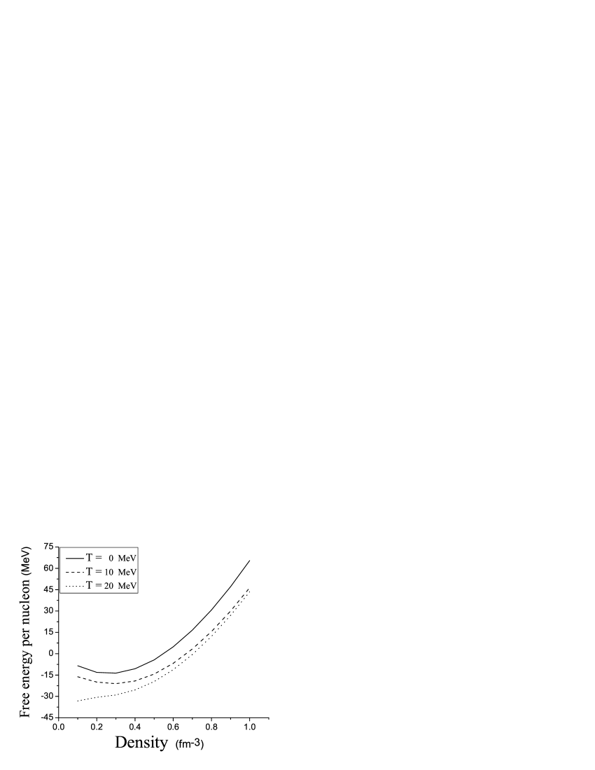
Figure 3: The free energy per nucleon of the nuclear matter versus the total number density ($\rho$) for unpolarized case at ${\cal T}=0$, $10$ and $20$ MeV .

The free energy per nucleon of the polarized hot nuclear matter versus the total number density ($\rho$) for different values of the spin polarization ($\delta$) at ${\cal T}=10$ and $20$ MeV is shown in Fig. 2. It can be seen that for each value of the temperature, the free energy increases by increasing both density and polarization. From Fig. 2, it is seen that the free energy of the polarized hot nuclear matter decreases by increasing the temperature. We have seen that above a certain values of the temperature and spin polarization, the free energy does not show any bound states for the polarized hot nuclear matter. From Fig. 2 we also see that for all given temperatures there is no crossing of the free energy curves for different polarizations and the difference between the free energy of the nuclear matter at different polarizations increases by increasing the density. This indicates that the spontaneous transition to the ferromagnetic phase does not occur in the hot nuclear matter. We have also compared the free energy per nucleon of the unpolarized case of the nuclear matter at different temperatures in Fig. 3. It is seen that the free energy of unpolarized nuclear matter decreases by increasing the temperature. We can see that above a certain temperature, the free energy does not show the bound state (the minimum point of the free energy) for the unpolarized nuclear matter.

For the polarized hot nuclear matter, the magnetic susceptibility, $\chi$, which characterizes the response of the system to the magnetic field can be calculated by using the following relation,

$$\chi=\frac{\mu^{2}\rho}{\left(\frac{\partial^{2}F}{\partial\delta^{2}}\right)_{\delta=0}},$$ (43)

where $\mu$ is the magnetic moment of the nucleons. Fig. 4 shows the ratio ${{\chi_{F}}/{\chi}}$ as a function of the temperature at $\rho=0.16fm^{-3}$, where $\chi_{F}$ is the magnetic susceptibility for a noninteracting Fermi gas. As it can be seen from this figure, this ratio is inversely proportional to absolute temperature without any anomalous change in its behavior. This indicates that hot nuclear matter is paramagnetic. The ratio ${{\chi_{F}}/{\chi}}$ has been also shown versus the total number density at temperature ${\cal T}=20$ MeV in Fig. 5. A magnetic instability would require ${{\chi_{F}}/{\chi}<0}$. It is seen that the value of ${{\chi_{F}}/{\chi}}$ is always positive and monotonically increasing up to highest density and does not show any spontaneous phase transition to the ferromagnetic phase for the hot nuclear matter.

The difference between the entropy per nucleon of the fully polarized and unpolarized cases of the nuclear matter is plotted as a function of the total number density at ${\cal T}=20$ MeV in Fig. 6. It is seen that for all given values of the density, this difference is negative. This shows that the fully polarized case of hot nuclear matter is more ordered than the unpolarized case. We also see that the magnitude of this deference decreases by increasing the density. The entropy per nucleon of the polarized hot nuclear matter versus the spin polarization for fixed density $\rho=0.5fm^{-3}$ and temperature ${\cal T}=20$ has been presented in Fig. 7. It is shown that the entropy decreases by increasing the polarization. It is also shown that the highest value of the entropy occurs for the unpolarized case of the hot nuclear matter. For the polarized hot nuclear matter, the following condition for the effective mass prevents the anomalous behavior of the entropy versus the spin polarization apv ,

$$\frac{m^{*}(\rho,\delta=1.0)}{m^{*}(\rho,\delta=0.0)}<2^{2/3},$$ (44)

where $m^{*}(\rho,\delta=1.0)$ and $m^{*}(\rho,\delta=0.0)$ are the effective masses of the fully polarized and unpolarized nuclear matter, respectively. This condition was first derived in Ref. apv for the particular case of the Skyrme interaction where the effective mass is independent of the momentum and temperature and therefore the single particle potential is purely parabolic. In our approach, the effective mass depends on both density and temperature but is independent of the momentum. In other words, a similar rigorous condition can not be obtained straightforwardly. However, within this approximation, one can use the condition of Eq. (44). From our result for the effective mass at ${\cal T}=20MeV$ for $\rho=0.5fm^{-3}$ (Fig. 1), we have found that this ratio is $1.24$. We see that this value is smaller than the above limiting value which indicates that the entropy of polarized case of the hot nuclear matter is always smaller than the entropy of unpolarized case. This so-considered ”natural” behavior was also found in the case of Gogny dapv and in the BHF analysis of Ref. bprrv . In contrast, for Skyrme forces the entropy per particle of the polarized phase is seen to be higher than the non-polarized one above a certain density dapv .

Finally, we have plotted the pressure of the polarized hot nuclear matter as a function of the total number density ($\rho$) for different polarizations at ${\cal T}=10$ and $20$ MeV in Fig. 8. For all values of temperature and polarization, it is seen that the pressure increases by increasing the density. For this system, we see that at each temperature the equation of state becomes stiffer as the polarization increases. For each polarization, it is found that the pressure of the polarized hot nuclear matter increases by increasing the temperature.

IV Summary and Conclusions

The lowest order constrained variational (LOCV) method has been used for calculating the susceptibility of the polarized hot nuclear matter and some of the thermodynamic properties of this system such as the effective mass, free energy, entropy and the equation of state. In our calculations, we have employed the $AV_{18}$ potential. Our results show that the spontaneous transition to the ferromagnetic phase does not occur for the hot nuclear matter. We have seen that the spin polarization substantially affects the thermodynamic properties of the hot nuclear matter.

Figure 1: The effective mass of spin-up (full curve) and spin-down (dashed curve) nucleons versus the spin polarization ($\delta$) for density $\rho=0.5fm^{-3}$ at ${\cal T}=20$ MeV.

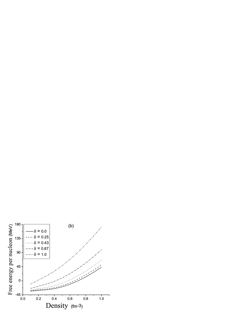
Figure 2: The free energy per nucleon of the polarized hot nuclear matter as a function of the total number density ($\rho$) for different values of the spin polarization ($\delta$) at ${\cal T}=10$ (a) and ${\cal T}=20$ MeV (b).

Figure 4: The magnetic susceptibility of the hot nuclear matter versus the temperature at $\rho=0.16fm^{-3}$ .

Figure 5: The magnetic susceptibility of the hot nuclear matter versus the total number density ($\rho$) at ${\cal T}=20$ MeV.

Figure 6: As Fig. 4 but for the entropy difference of the fully polarized and the unpolarized cases.

Figure 7: The entropy per nucleon as a function of the spin polarization ($\delta$) for density $\rho=0.5fm^{-3}$ at ${\cal T}=20$ MeV .

Figure 8: The equation of state of the polarized hot nuclear matter for different values of the spin polarization ($\delta$) at ${\cal T}=10$ (a) and ${\cal T}=20$ MeV (b).