Thermodynamics of charged black holes with a nonlinear electrodynamics source

Abstract

We study the thermodynamical properties of electrically charged black hole solutions of a nonlinear electrodynamics theory defined by a power $p$ of the Maxwell invariant, which is coupled to Einstein gravity in four and higher spacetime dimensions. Depending on the range of the parameter $p$, these solutions present different asymptotic behaviors. We compute the Euclidean action with the appropriate boundary term in the grand canonical ensemble. The thermodynamical quantities are identified and in particular, the mass and the charge are shown to be finite for all classes of solutions. Interestingly, a generalized Smarr formula is derived and it is shown that this latter encodes perfectly the different asymptotic behaviors of the black hole solutions. The local stability is analyzed by computing the heat capacity and the electrical permittivity and we find that a set of small black holes are locally stable. In contrast to the standard Reissner-Nordström solution, there is a first-order phase transition between a class of these non-linear charged black holes and the Minkowski spacetime.

I Introduction

The nonlinear electrodynamics models have been proved to be excellent laboratories in order to circumvent some problems that occur in the standard Maxwell theory. Indeed, the interest for nonlinear electrodynamics has started with the precursor work of Born and Infeld, whose main motivation was to modify the standard Maxwell theory in order to eliminate the problem of infinite energy of the electron Born:1934gh . However, due to the fact that the Born-Infeld model did not fulfill all the hope, nonlinear electrodynamics theories become less popular. The recent renewal interest on the nonlinear electrodynamics theories is essentially due to their emergence in the context of low-energy limit of heterotic string theory, where a Gauss-Bonnet term coupled to quartic contractions of Maxwell field strength appear, and black hole solutions can be obtained HF . It is also important to mention that nonlinear electrodynamics theories are a powerful tool for the construction of regular black hole solutions regularBH .

The thermodynamics properties of nonlinear electrodynamics theories is also an active research area in the current literature, see e.g. examplesTherm in the case of the Born-Infeld model. A very appealing property which is common to all the nonlinear electrodynamic models lie in the fact that these theories satisfy the zeroth and first law of black hole mechanics Rasheed:1997ns . This property renders more attractive the studies of nonlinear electrodynamics models. However, in contrast with the standard Maxwell theory, the formula of the total mass, the so-called Smarr formula Smarr:1972kt , does not hold a priori for nonlinear electrodynamic theories Rasheed:1997ns . Indeed, in the case of the Einstein-Maxwell system, the Smarr formula and the first law of black holes mechanics are closely related and each of them can be derived from the other. This correspondence between both formulas is due to the homogeneity of the mass in terms of the area of the horizon and the electric charge Gibbons:1976pt ; Gauntlett:1998fz . However, in the case of nonlinear electrodynamic theories, this homogeneity property is not longer present and there is a priori no good reason to obtain a Smarr formula. Some attempts to generalize the Smarr formula in order to be in accordance with the variations expressed by the first law of black holes mechanics have shown to be possible for some particular magnetic solutions in four dimensions Breton:2004qa . For completeness, we stress that the derivation of the Smarr formula as well as of the first law of thermodynamics are usually performed successfully for asymptotically flat spacetime through the Komar integrals Bardeen:1973gs . However, their extension to rotating asymptotically anti-de Sitter black hole solutions is not a simple task as it can be seen by reading the current literature on the topic Gibbons ; Barnich:2004uw .

In the present paper, we consider higher-dimensional gravity coupled to a nonlinear electrodynamic source given by a rational power $p$ of the Maxwell invariant. This theory exhibits electrically charged black hole solutions as long as the exponent $p$ belongs to the set of rational number with odd denominator Hassaine:2007py ; Hassaine:2008pw . Similar considerations and motivations were previously analyzed in three dimensions in Cataldo:2000we . Recently, this nonlinear model has attracted attention, and it has been used for obtaining Lovelock black holes Hideki , Ricci flat rotating black branes Hendi1 , magnetic strings Hendi2 and topological black holes in Gauss-Bonnet gravity Hendi3 . A generalization of this model for the non abelian case was considered in Mazharimousavi:2009mb . The black hole solutions derived in Hassaine:2008pw are divided in four ranges for the exponent $p$, and each of them correspond to a different spacelike asymptotic behavior of the metric. Among these different classes, there exist black hole solutions with unusual asymptotic properties as those that go asymptotically to the Minkowski spacetime slower than the Schwarzschild spacetime. There also exists a range for $p$ for which the solutions are not asymptotically flat and, their asymptotic behavior is shown to grow slower that the Schwarzschild de Sitter spacetime. Extremal black hole solutions generalizing the extremal Reissner-Nordström solution are also known for this model Hassaine:2008pw .

The main objective here is to provide a detailed analysis of the thermodynamical properties of these black hole solutions. In particular, we would like to explore the relation between the thermodynamical properties and the different asymptotic behaviors of the solutions. The thermodynamics of the electrically charged black hole solutions will be performed through the Regge-Teitelboim approach Regge:1974zd , in which an appropriate boundary term is added to the Euclidean action such that the total action presents an extremum. On the other hand, owing to the fact that the Euclidean action is related to the Gibbs free energy, the identification of the mass and the charge, as well as the study of the global stability of the black holes will be considerably facilitated. We will derive a generalized Smarr formula by using the explicit expressions of the temperature and the entropy. Interesting enough, we will show that the different asymptotic behaviors of the black hole solutions are reflected through this Smarr formula. In addition, we will present two other different ways of obtaining of the Smarr formula. The first derivation is operated through the Komar integrals for all the class of solutions even those that are not asymptotically flat. The same formula will also be obtained with the use of a Noether conserved current which is associated to a scale symmetry of the reduced action. The local stability of the black holes are analyzed by computing the heat capacity and the electrical permittivity. For a certain range of the exponent $p$, small black hole solutions with positive and negative mass will be shown to be locally stable. Finally, the global stability is studied through the Gibbs free energy in order to determine whether the electrically charged black hole solutions are most likely than the Minkowski background. As a result, we will establish that there exists a phase transition for a certain range of the exponent $p$.

The plan of the paper is organized as follows. In the next section, we review the nonlinear electrodynamics model and its general black hole solutions Hassaine:2008pw . In Sec. III, the thermodynamics properties of the system are studied through the Euclidean Hamiltonian formalism. The mass $M$ and the charge $Q$ are explicitly identified and a generalized Smarr formula is derived. In Sec. IV the local and global stability of these black holes is analyzed, while the last section is devoted to the conclusions and further prospects. Finally, two appendices are devoted to the different derivations of the Smarr formula.

II Nonlinear electrodynamics and black hole solutions

In Hassaine:2007py ; Hassaine:2008pw , a nonlinear electrodynamics coupled to gravity in $d$ spacetime dimensions was considered. This model is described by the action

$$I[g_{\mu\nu},A_{\mu}]=\int d^{d}x\sqrt{-g}\left(\frac{R}{2\kappa}-\alpha\left(F_{\mu\nu}F^{\mu\nu}\right)^{p}\right),$$ (1)

where $\kappa$ denotes the gravitational constant, $\alpha$ the coupling constant for the electrodynamical action, $F_{\mu\nu}=\partial_{\mu}A_{\nu}-\partial_{\nu}A_{\mu}$ is the field strength and $p$ is a rational number whose range will be fixed later. The field equations obtained by varying this action are given by

$$G_{\mu\nu}=4\kappa\alpha\left[p\,F_{\mu\rho}F_{\nu}^{\,\,\,\rho}\,F^{p-1}-\frac{1}{4}g_{\mu\nu}\,F^{p}\right],$$ (2a)

$$\partial_{\mu}\left(\sqrt{-g}\,F^{\mu\nu}\,F^{p-1}\right)=0,$$ (2b)

where $F=F_{\alpha\beta}F^{\alpha\beta}$ is the Maxwell invariant. The most general spherically symmetric solution with a radial electric field was found in Hassaine:2007py for the conformal case $p=d/4$, and in Hassaine:2008pw for $p$ belonging to the set of rational numbers with odd denominators. The general solution is described by the line element

$$ds^{2}=-N^{2}(r)f^{2}(r)dt^{2}+{\frac{dr^{2}}{f^{2}(r)}}+r^{2}d\Omega_{d-2}^{2},$$ (3)

with

$$N^{2}(r)=1,$$ (4a)

$$f^{2}(r)=1-\frac{A}{r^{d-3}}+\frac{B}{r^{b}},$$ (4b)

$$F_{tr}=\frac{C}{r^{\frac{d-2}{2p-1}}},$$ (4c)

where for convenience we have defined

$$B=-\frac{2\kappa\alpha(-1)^{p}C^{2p}2^{p}(2p-1)^{2}}{(d-2)(d-2p-1)},\qquad\quad b=\frac{2(pd-4p+1)}{2p-1}.$$ (5)

These solutions contain black hole configurations depending on the values of $d$ and $p$, and the integration constants $A$ and $C$.

Apart from the restriction of being a rational numbers with odd denominators, the exponent $p$ can not belong to the set $(0,1/2]$ since in this case the scalar curvature of the solutions diverges at the infinity. The form of the lapse function suggests a natural partition depending on the exponent $b$ that appears in (4b). These different ranges are given by $b>d-3$, $0<b<d-3$, $b<0$, and $b=d-3$, which correspond to the different spacelike asymptotic behaviors of the metric, as it is shown in Table I. Solutions of type I have a behavior similar to the standard Reissner-Nordström one. By similar, we mean that the charge term in the metric decays faster than the mass term in the asymptotic region. At the opposite, solutions of type II correspond to black hole solutions which go asymptotically to the Minkowski spacetime slower than the Schwarzschild spacetime. In the case III, the black hole solutions are not asymptotically flat, and their asymptotic behavior is shown to grow slower that the Schwarzschild de Sitter spacetime. Finally, the critical value $b=d-3$, which can only occur for odd dimensions $d=2p+1$, corresponds to the limit between the solutions which resemble to the standard Reissner-Nordström solution (type I) and those for which the asymptotic decaying to Minkowski spacetime are slower than the Schwarzschild spacetime (type II). The spherically symmetric solution in this special case involves a logarithmic dependance on the radial coordinate and is given by

$$F_{tr} = \frac{C}{r},$$ (6a)

$$f^{2}(r) = 1-\frac{A}{r^{2p-2}}+\kappa\alpha(-1)^{p}2^{p+1}C^{2p}\frac{\ln r}{r^{2p-2}}.$$ (6b)

Type	$b$	$p$	Remarks
I	$b>d-3$	$1/2<p<(d-1)/2$	Standard asymptotically flat case
II	$0<b<d-3$	$p>(d-1)/2$ or $p<-1/(d-4)$	Electric term with relaxed fall-off
III	$b\leq 0$	$-1/(d-4)\leq p<0$	Asymptotically non-flat case
Log	$b=d-3$	$p=(d-1)/2$ with $d$ odd	Logarithmic case

Table 1: Classification of the solutions depending on its asymptotic behavior. The cases are labeled in the first column. In the second column the different cases are defined by the parameter $b$ and, equivalently by $p$, in the third column. In the last column we describe the main spacelike asymptotic feature for each case.

III Thermodynamics

It is well known that the partition function for a thermodynamical ensemble can be identified with the Euclidean path integral in the saddle point approximation around the Euclidean continuation of the classical solution Gibbons:1976ue . In this case, the Euclidean action $I_{E}$ evaluated on the classical solution is related to the free energy $G$ of a thermodynamical ensemble by $I_{E}=\beta G$, where $\beta$ is the inverse of the temperature which corresponds to the period of the Euclidean time $\tau$.

As a first step we write the action in the Hamiltonian form, and since we are concerned only with the static, spherically symmetric case without magnetic field, it is enough to consider a reduced action principle. The class of the Euclidean metric and electric potential to be considered are given by

$$ds^{2}=N(r)^{2}f(r)^{2}d\tau^{2}+\frac{dr^{2}}{f(r)^{2}}+r^{2}d\Omega_{d-2}^{2},\qquad\quad\quad A=A(r)d\tau,$$

where the radial coordinate $r$ belongs to $[r_{+},\infty)$. In this case, the Euclidean reduced action obtained from (1) reads

$$I_{E}=-\beta\;\Omega_{d-2}\int_{r_{+}}^{\infty}dr\left\{\frac{(2p-1)\alpha N(-2)^{\frac{p}{2p-1}}}{r^{\frac{d-2}{2p-1}}}\left(\frac{{\cal P}}{4\alpha p}\right)^{\frac{2p}{2p-1}}-\frac{d-2}{2\kappa}Nr^{d-2}\left[\frac{(f^{2})^{\prime}}{r}-\frac{d-3}{r^{2}}(1-f^{2})\right]+\phi{\cal P}^{\prime}\right\}+K,$$ (7)

where ${\cal P}\equiv 4\alpha p\,N_{\infty}\,r^{d-2}F^{p-1}F^{rt}$ is the rescaled canonical radial momentum, $\phi\equiv A(r)$ is the electrostatic potential, $\Omega_{d-2}$ is the area of the $d-2$-dimensional unit sphere. The boundary term $K$ appearing in (7) will be fixed by requiring that the action has an extremum on-shell Regge:1974zd . Moreover, owing to the fact that the Hamiltonian action is a linear combination of the constraints, the value on the action on-shell is given by the boundary term $K$.

The equations of motion obtained by varying the reduced action with respect to $N$, $f^{2}$, ${\cal P}$ and $\phi$ are given by

$$\frac{(f^{2})^{\prime}}{r}-\frac{d-3}{r^{2}}(1-f^{2})=\frac{2\kappa\alpha(2p-1)}{d-2}\frac{(-2)^{\frac{p}{2p-1}}}{r^{\frac{2p(d-2)}{2p-1}}}\left(\frac{{\cal P}}{4\alpha p}\right)^{\frac{2p}{2p-1}},$$ (8a)

$$N^{\prime}=0,$$ (8b)

$$\phi^{\prime}=\frac{N(-2)^{\frac{p}{2p-1}}}{2r^{\frac{d-2}{2p-1}}}\left(\frac{{\cal P}}{4\alpha p}\right)^{\frac{1}{2p-1}},$$ (8c)

$${\cal P}^{\prime}=0.$$ (8d)

Note that these equations are consistent with the original Einstein equations (2). The general solution reads

$$f^{2}(r) = \left\{\begin{array}[]{lll}\displaystyle 1-\frac{A}{r^{d-3}}+\frac{B}{r^{b}},&\mbox{if}&b\neq d-3.\\ &&\\ 1-\frac{A}{r^{2p-2}}+\kappa\alpha(-1)^{p}2^{p+1}C^{2p}\frac{\ln r}{r^{2p-2}},&\mbox{if}&b=d-3,\end{array}\right.$$ (9d)

$$N(r) = N_{\infty}$$ (9e)

$$\phi(r) = \left\{\begin{array}[]{lll}\displaystyle\frac{2p-1}{d-2p-1}\frac{N_{\infty}C}{r^{\frac{d-2p-1}{2p-1}}}+\phi_{0},&\mbox{if}&b\neq d-3.\\ &&\\ -N_{\infty}C\ln(r)+\phi_{0},&\mbox{if}&b=d-3,\end{array}\right.$$ (9i)

$${\cal P}(r) = {\cal P}_{0}$$ (9j)

where $N_{\infty}$, ${\cal P}_{0}$ , $A$ and $\phi_{0}$ are integration constants (without loss of generality, we can set $N_{\infty}=1$ and $\phi_{0}=0$), and where we have defined

$$B=-\frac{2\kappa\alpha(-2)^{\frac{p}{2p-1}}(2p-1)}{(d-2)(d-2p-1)}\left(\frac{{\cal P}_{0}}{4\alpha p}\right)^{\frac{2p}{2p-1}}\quad\mbox{and}\quad C=(-2)^{\frac{1-p}{2p-1}}\left({\cal P}_{0}\right)^{\frac{1}{2p-1}}({4\alpha p})^{\frac{1}{1-2p}}.$$ (10)

In what follows, we consider the formalism of the grand canonical ensemble, and hence we will consider the variation of the action keeping fixed the temperature $\beta^{-1}$ and the electric potential, $\Phi=\phi(r_{+})$. This variation gives bulk terms proportional to the constraints, some surface terms and the variation $\delta K$. As we shall see, the requirement that the action has an extremum, i. e. $\delta I_{E}=0$ on-shell, will fix properly the boundary term. The condition $\delta I_{E}=0$ implies that the variation of the boundary term, which cancels out the extra surface terms coming from variation of the action is given by

$$\delta K=\beta\;\Omega_{d-2}\left[-\frac{d-2}{2\kappa}Nr^{d-3}\delta f^{2}+\phi\delta{\cal P}\right]_{r_{+}}^{\infty}\equiv\delta K({\infty})-\delta K({r_{+}}),$$ (11)

Since the metric solution $f^{2}(r)$ differs drastically for $b\neq d-3$ and $b=d-3$, we shall consider both cases separately. Interesting enough, we shall see that in both cases, the apparently divergent contributions at the infinity will cancel yielding to a finite and same expression in these two distinct cases.

For $b\neq d-3$, the variations of the fields at infinity ($r\rightarrow\infty$) are given by

$$\delta f^{2}|_{\infty} = -r^{-(d-3)}\delta A+r^{-b}\delta B,$$ (12)

$$\delta{\cal P}|_{\infty} = \delta{\cal P}_{0},$$ (13)

and hence we have

$$\delta K({\infty})=\beta\;\Omega_{d-2}\left[\frac{d-2}{2\kappa}\delta A+\left(-\frac{d-2}{2\kappa}\delta B+\frac{2p-1}{d-2p-1}C\delta{\cal P}_{0}\right)r^{d-3-b}\right].$$ (14)

For $b<d-3$, the contribution proportional to $r^{d-3-b}$ may blow up at infinity, but since the factor between round brackets multiplying this term identically vanishes, the variation of the boundary term at infinity yields to a finite expression given by

$$\delta K({\infty})=\frac{d-2}{2\kappa}\beta\;\Omega_{d-2}\delta A.$$ (15)

For the case $b=d-3$, which corresponds to an exponent $p=(d-1)/2$, we have a similar derivation. Indeed, the variations of the fields at infinity read

$$\delta f^{2}|_{\infty} = -r^{-(d-3)}\delta A+\kappa\alpha(-1)^{p}2^{p+1}\delta C^{2p}r^{-(d-3)}\ln(r),$$ (16)

$$\delta{\cal P}|_{\infty} = \delta{\cal P}_{0},$$ (17)

and hence,

$$\delta K({\infty})=\beta\;\Omega_{d-2}\left[\frac{d-2}{2\kappa}A-\Big{(}(d-2)\alpha(-1)^{p}2^{p}\delta C^{2p}+C\delta{\cal P}_{0}\Big{)}\ln(r)\right].$$ (18)

As in the previous case, since the following equality $(d-2)\alpha(-1)^{q}2^{q}\delta C^{2q}+C\delta{\cal P}_{0}=0$ holds for $p=(d-1)/2$, the logarithmic dependance disappears yielding to the same variation (15). We conclude that in both cases, the integration of the variation (15) leads to a finite expression given by

$$K({\infty})=\frac{d-2}{2\kappa}\beta\Omega_{d-2}A.$$ (19)

In order to evaluate the variation of the metric function $f^{2}(r)$ at the horizon $r_{+}$, we use the fact that the solution satisfies $f^{2}(r_{+})=0$ together with the condition that ensure the absence of conical singularities at the horizon, that is $(f^{2})^{\prime}|_{r_{+}}=4\pi/\beta$. This condition fixes the temperature of the ensemble while the electric potential $\phi$ and the variation of ${\cal P}$ are evaluated directly,

$$\delta f^{2}|_{r_{+}} = -(f^{2})^{\prime}|_{r_{+}}\delta{r_{+}}=-\frac{4\pi}{\beta}\delta{r_{+}},$$ (20)

$$\phi\,\delta{\cal P}|_{r_{+}} = \phi(r_{+})\delta{\cal P}_{0}.$$ (21)

The variation of the boundary term is easily integrated at the horizon yielding

$$K({r_{+}})=-\Phi\beta{\cal P}_{0}\Omega_{d-2}+\frac{2\pi}{\kappa}\Omega_{d-2}r_{+}^{d-2}.$$

Finally, the on-shell Euclidean action, which reduces to the boundary term $K=K({\infty})-K({r_{+}})$, reads

$$I_{E}=\beta\frac{d-2}{2\kappa}\Omega_{d-2}A-\beta\Phi{\cal P}_{0}\Omega_{d-2}-\frac{2\pi}{\kappa}\Omega_{d-2}r_{+}^{d-2}.$$ (22)

As it will be shown below, this expression is useful in order to identify the thermodynamical quantities and in the study of the global stability of the black hole solutions. Indeed, the Euclidean action is related to the Gibbs free energy by $I_{E}=\beta G=\beta M-\beta\Phi Q-S$. This relation allows to easily identify the mass ($M$), the electric charge ($Q$) and the entropy ($S$) as

$$M = \left(\frac{\partial I_{E}}{\partial\beta}\right)_{\Phi}-\frac{\Phi}{\beta}\left(\frac{\partial I_{E}}{\partial\Phi}\right)_{\beta}=\frac{(d-2)\Omega_{d-2}}{2\kappa}A,$$ (23a)

$$Q = -\frac{1}{\beta}\left(\frac{\partial I_{E}}{\partial\Phi}\right)_{\beta}=\Omega_{d-2}{\cal P}_{0},$$ (23b)

$$S = \beta\left(\frac{\partial I_{E}}{\partial\beta}\right)_{\Phi}-I_{E}=\frac{2\pi}{\kappa}\Omega_{d-2}r_{+}^{d-2}.$$ (23c)

As a first and direct consequence, these quantities must satisfy the first law of thermodynamics $\delta M=T\delta S+\Phi\delta Q$ which is indeed the case. In a more unexpected way, these expressions (23) permit to derive a generalized Smarr formula. In order to achieve this task, we first express the event horizon radius in terms of the thermodynamical quantities (23) as

$$r_{+}^{d-3}=\frac{2\kappa M}{\Omega_{d-2}(d-2)}-\frac{\kappa(2p-1)}{\Omega_{d-2}p(d-2)}Q\Phi.$$ (24)

Throughout this relation, the entropy and the temperature can be written as

$$S = 4\pi\left(\frac{2\kappa}{\Omega_{d-2}[2p\left(d-2\right)]^{d-2}}\right)^{\frac{1}{d-3}}\left[2pM-\left(2p-1\right)Q\Phi\right]^{\frac{d-2}{d-3}},$$

$$T = \frac{1}{4\pi}\left(\frac{p\Omega_{d-2}(d-2)}{\kappa}\right)^{\frac{1}{d-3}}\frac{2Mp(d-3)-2(pd-4p+1)Q\Phi}{\left(2pM-(2p-1)Q\Phi\right)^{\frac{d-2}{d-3}}}.$$

Remarkably enough, multiplying these two expressions and, after some algebraic manipulations, we obtain a formula for the total mass given by

$$M=\frac{d-2}{d-3}ST+\frac{pd-4p+1}{p\left(d-3\right)}Q\Phi,$$ (25)

which is nothing but a Smarr formula. We first observe that for $p=1$, the relation (25) reduces to the well-known Smarr formula for the $d-$dimensional Einstein-Maxwell black holes Gauntlett:1998fz . Another interesting value of the exponent is given by $p=1/(4-d)$ for which the contribution of the charge in the formula (25) disappears and the formula is similar to the Smarr formula for the Schwarzschild solution. This is not surprising since in this case, the charge contribution in the metric (see (4b) and (5)) becomes constant and hence, the solution resembles to the Schwarzschild metric but with a deficit solid angle. In fact, this critical value of $p$ corresponds to the transition between the solutions which asymptote the Minkowski spacetime (type II) and those that go slowly than the Schwarzschild de-Sitter solutions, i. e. $f^{2}(r)\sim r^{-b}$ with $0<-b<2$ (type III). This peculiar transition is also reflected in the total mass formula (25) by the fact that the term proportional to the charge changes its sign. More precisely, the sign of the term proportional to the charge in the case of solutions of type II is opposite to the sign relative of those of type III, and the transition is precisely operated at the critical value $p=1/(4-d)$. Another value to consider is $p=0$ because of the apparent singularity of the formula (25). However, a detailed analysis shows that for $p=0$ the formula reduces to the standard Smarr formula for the Schwarzschild-(anti) de Sitter metric (with a cosmological constant $\Lambda=\kappa\alpha$),

$$M=\frac{d-2}{d-3}ST+\frac{2\alpha\Omega_{d-2}}{(d-3)(d-1)}\left.r_{+}^{d-1}\right|_{p=0},$$

where the expression of the horizon radius (24) is evaluated at $p=0$. This is not surprising since at the level of the action, the value $p=0$ turns to be equivalent of having the Einstein action with a cosmological constant. Within this detailed study of the expression (25), we have pointed out that the Smarr formula by its own reflects the different asymptotic behaviors of the black hole solutions. Finally, we mention that the Smarr law can also be derived in two different other manners: by using the Komar integral even in the cases of the non asymptotic flat solutions, (see Appendix A1) or by constructing a Noether conserved current which is associated to a scaling symmetry of the reduced action (7), see Appendix A2.

For latter convenience, we now express the mass and the temperature in terms of the horizon $r_{+}$. Since we are working in the grand canonical ensemble, these expressions must be written in terms of the fixed state variables, namely the potential $\Phi$ and the temperature $T$. A straightforward computation shows that the mass $M$ expressed as a function of $r_{+}$ reads

$$M=\frac{\Omega_{d-2}(d-2)}{2\kappa}\left[r_{+}^{d-3}+\frac{(2p-1)D}{d-2p-1}r_{+}^{d-2p-1}\right].$$ (26)

This relation is useful to analyze the behavior of the mass with respect to the event horizon radius for the different classes of solutions, cf. Fig. 1.

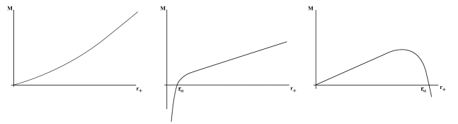
Figure 1: Mass of the black hole in terms of the event horizon radius $r_{+}$ at fixed electric potential $\Phi$. The first graph corresponds to the solutions with $p\in\left(\frac{1}{2},\frac{d-1}{2}\right)$, while the second one represents the solutions with $p>\frac{d-1}{2}$. The last graph is identified with the solutions with a negative exponent $p<0$. For the two first graphs ($p>1/2$), the mass is a monotonous function of the horizon radius, with the particularity that black hole solutions with negative mass are only allowed for $p>(d-1)/2$. This fact occurs when $r_{+}<r_{\rm M}$, where $r_{\rm M}$ corresponds to the radius for which the mass vanishes. In contrast, for $p<0$ the mass is not a monotonous function and has a local maximum, as it is shown in the last graph. Moreover, in the range ${1}/(4-d)<p<0$, only black hole solutions with positive mass can be exhibited, since for this interval of $p$ the negative mass solutions have a negative temperature (see Fig. 2). For the remaining range $p<1/(4-d)$, the mass can be negative since its corresponding temperature is positive.

On the other hand, the square temperature is given by

$$T^{2} = \left[\frac{1}{4\pi}\left.\frac{df^{2}}{dr}\right|_{r+}\right]^{2},$$

which, after some algebraic manipulations, can be rewritten as

$$T^{2}=\left[\frac{1}{4\pi}\left(\frac{d-3}{r_{+}}-\frac{D}{r_{+}^{2p-1}}\right)\right]^{2},$$ (27)

and where the constant $D$ is given by

$$D=-2\kappa\alpha(-2)^{p}(d-2)^{-1}(2p-1)^{1-2p}(d-2p-1)^{2p}\Phi^{2p}.$$

It is important to mention that, due to the positive energy condition Hassaine:2008pw , the constant $D$ is positive for all the values of the exponent $p$. For clarity, in Fig. 2, we sketch the temperature as a function of the horizon radius for the different range of the parameter $p$.

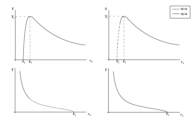
Figure 2: Temperature against the horizon $r_{+}$ for different ranges of the exponent $p$ at fixed electric potential $\Phi$. At the top left, the graph corresponds to the range $p\in(\frac{1}{2},\frac{d-1}{2})$, while the top right graph represents the solutions with $p>\frac{d-1}{2}$. The last graphs are respectively for $p<\frac{1}{4-d}$ and $p\in(\frac{1}{4-d},0)$. For the exponent $p$ ranging over the set $(\frac{1}{2},\frac{d-1}{2})$, the asymptotic behavior of the solution is similar to the Reissner-Nordström black hole, and the analogy is also valid concerning the thermodynamics. In particular, for large value of the horizon, the temperature goes to zero while it reaches its maximum $T_{0}$ for a finite value of the horizon radius $r_{0}$. In addition, there exists a value $r_{\rm T}$ for which the temperature vanishes, which corresponds to an extremal black hole. For $p>(d-1)/2$, the main difference with the previous case lies in the fact that there exist black holes with positive and negative mass, and the extremal solution is possible only for negative mass. For $p<1/(4-d)$, the temperature behavior is quite different since it is a decreasing function of the event horizon, and as before, the extremal solution is possible only with a negative mass. Finally, for $1/(d-4)<p<0$, the temperature is similar to the previous case, with the exceptions that the mass is always positive, and the value for which the temperature vanishes does not correspond to an extremal black hole.

IV Local and global thermodynamic stability

The thermodynamic stability of a system can be considered from many different point of views depending on which thermodynamical variables or state functions one is considering. Usually, in order to study the stability of a system, it is common to consider small fluctuations of the state functions around the equilibrium, and since the first order terms vanish, the stability is only a statement about the second order variations. An equivalent manner of studying the local stability can be done by analyzing the sign of the heat capacity $C_{\Phi}$ at constant potential

$$C_{\Phi}\equiv T\left(\frac{\partial S}{\partial T}\right)_{\Phi},$$ (28)

as well as, the sign of the electrical permittivity $\epsilon_{T}$ at constant temperature

$$\epsilon_{T}\equiv\left(\frac{\partial Q}{\partial\Phi}\right)_{T}.$$ (29)

From these definitions, it is clear that the heat capacity (resp. the electrical permittivity) gives information about the thermal stability with respect to the temperature fluctuations (resp. to the electrical fluctuations). The positivity of the heat capacity, $C_{\Phi}\geq 0$, is a necessary condition for the system to be locally stable and, this is a direct consequence of the definition (28) and the fact that the entropy is proportional to the size of the black hole Chamblin:1999hg . On the other hand, the black holes will be electrically unstable under electrical fluctuations if the electrical permittivity is negative. The physical interpretation of this instability is explained by the fact that in this case the potential decreases while the system acquires more charge, and hence the system may leave easily the equilibrium state Chamblin:1999hg . The local stability of a system will be ensured only if there exists a range of the horizon radius for which the quantities $C_{\Phi}$ and $\epsilon_{T}$ are both positives.

In order to express the heat capacity (28) as well as the electrical permittivity (29) in terms of the horizon radius, we rewrite them as

$$C_{\Phi}=T\left(\frac{\partial T}{\partial r_{+}}\right)^{-1}_{\Phi}\left(\frac{\partial S}{\partial r_{+}}\right)_{\Phi}=-\frac{2\pi}{\kappa}\Omega_{d-2}(d-2)r_{+}^{d-2}\left(\frac{D-(d-3)r_{+}^{2p-2}}{(2p-1)D-(d-3)r_{+}^{2p-2}}\right),$$ (30)

and

$$\epsilon_{T}=\left(\frac{\partial\Phi}{\partial r_{+}}\right)_{T}^{-1}\left(\frac{\partial Q}{\partial r_{+}}\right)_{T}.$$

However, since we have only the dependence of the charge $Q$ in terms of the potential at constant horizon, we have to rewrite each factor of the above formula as

$$\left(\frac{\partial Q}{\partial r_{+}}\right)_{T}=-\left(\frac{\partial T}{\partial Q}\right)_{r_{+}}^{-1}\left(\frac{\partial T}{\partial r_{+}}\right)_{Q},$$

$$\left(\frac{\partial\Phi}{\partial r_{+}}\right)_{T}=-\left(\frac{\partial T}{\partial\Phi}\right)_{r_{+}}^{-1}\left(\frac{\partial T}{\partial r_{+}}\right)_{\Phi}.$$

Combining these last expressions, the permittivity is found to be

$$\epsilon_{T} = \left(\frac{\partial Q}{\partial\Phi}\right)_{r_{+}}\left(\frac{\partial T}{\partial r_{+}}\right)_{\Phi}^{-1}\left(\frac{\partial T}{\partial r_{+}}\right)_{Q}$$ (31)

$$= -\frac{p(d-2)D}{\kappa\Phi^{2}(d-2p-1)}\Omega_{d-2}r_{+}^{d-2p-1}\left(\frac{(2pd-6p+1)D-(2p-1)(d-3)r_{+}^{2p-2}}{(2p-1)D-(d-3)r_{+}^{2p-2}}\right).$$

From the above formulas (30) and (31), it is clear that there is a strong influence of the exponent $p$ on the sign of these two expressions. Moreover, for a positive exponent $p$, both expressions will diverge at certain value of horizon radius $r_{0}$, reflecting a radical change in the thermodynamical local stability of the system. Indeed, the sign of the specific heat and electrical permittivity is flipped at $r_{0}$. For these reasons, it is interesting to plot $C_{\Phi}$ as well as $\epsilon_{T}$ against the event horizon $r_{+}$ for the different ranges of the exponent $p$.

Figure 3: Specific heat at fixed potential with $p\in(\frac{1}{2},\frac{d-1}{2})$, $p>\frac{d-1}{2}$ and $p<0$.

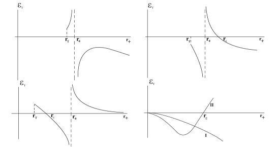
Figure 4: The electrical permittivity against $r_{+}$ for $p\in(\frac{1}{2},1)$, $p\in(1,\frac{d-1}{2})$ and $p>\frac{d-1}{2}$. For $p<0$ , there are two branches: the branch I corresponds to $p>\frac{1}{2(3-d)}$ while the branch II is relative to $p<\frac{1}{2(3-d)}$.

For the range $p\in(1/2,(d-1)/2)$, there exist only black holes with positive mass. In this case, the heat capacity (cf. Fig. 3) for $p\not=1$ have a positive and negative branches and present a vertical asymptote at $r_{0}$. For black hole with horizon $r_{+}\in(r_{T},r_{0})$, the heat capacity is positive, and hence the stability of the black hole is ensured for the thermal fluctuations. At the Reissner-Nordström limit, i.e. $p=1$, the singularity disappears and the heat capacity is always negative reflecting the instability of the solution. For the electrical permittivity (cf. Fig. 4), the analysis is divided in two parts. For $p\in(1/2,1)$ and for the region $r_{+}\in(r_{T},r_{0})$, the permittivity is positive and hence we conclude that the system is locally stable. In contrast, for $p\in(1,(d-1)/2)$ the system is unstable since there are no common regions where the heat capacity and the permittivity are both positive. For $p>(d-1)/2$, only small black hole with $r_{+}\in(r_{T},r_{\epsilon})$ and with negative mass are locally stable. Finally for $p<0$, independently of the sign of the mass, the solution is always unstable since the heat capacity is negative and hence the system is locally unstable. The main result is that the nonlinear electrodynamics theory considered in this paper permits the existence of locally stable black hole solutions. This result emphasizes the importance plays by the nonlinearity and is put in opposition with the local thermal instability of the standard Reissner-Nordström black hole.

We now turn to the study of the global stability in order to determine whether our solutions are thermodynamically preferred over the Minkowski background. The Gibbs free energy $G=I_{E}/\beta$ is an appropriate state function to compare configurations in the grand canonical ensemble. For example, it is well-known that in the standard Einstein-Maxwell theory, the Minkowski spacetime is always favored over the Reissner-Nordström black hole since in this case the free energy of this latter is positive.

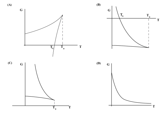
Figure 5: The Gibbs free energy in terms of temperature for $p\in(\frac{1}{2},1)$, $p\in(1,\frac{d-1}{2})$, $p>\frac{d-1}{2}$ and $p<0$ at fixed electric potential $\Phi$. A first-order phase transition can be observed only in the first graph at the temperature $T_{G}$.

In our case (cf. Fig 5) and for $p<0$, since the temperature is a monotonous function of the event horizon radius, the free energy is a positive decreasing function and hence the Minkowski background is more likely than the black hole configurations. For $p>(d-1)/2$ and for a fixed temperature two black hole configurations with different free energy and size coexist. In this case, in spite of the fact that both solutions are less likely than the Minkowski background, there is a non-vanishing probability that the black hole with the larger $r_{+}$ decays into the smaller one. In the case where the parameter $p\in(1/2,1)$ and for the temperature $T<T_{G}$, the larger black holes are thermodynamically preferred over the Minkowski background, and since for $T>T_{G}$ the black hole branch has a larger free energy than the Minkowski spacetime a first-order phase transition occurs at $T=T_{G}$. The situation is drastically different for $p\in(1,\frac{d-1}{2})$. Indeed, in this case the most probable configuration is that concerned with the small black hole branch, but in this case, phase transitions are not observed.

V Conclusions and comments

We have studied the thermodynamical properties of black hole arising as solutions of higher-dimensional gravity coupled to a nonlinear electrodynamics theory given as a power $p$ of the Maxwell invariant. These solutions have the peculiarity of having different asymptotic behaviors depending mainly on the range of the exponent $p$, including non asymptotically flat spacetimes. Metrics with asymptotic relaxed fall-off has attracted much attention slowfall for AdS gravity coupled to a scalar field with mass at or slightly above the Breitenlohner-Freedman bound BF . This theory allows a large class of asymptotically AdS spacetimes where the charges can be properly defined. In the present work we have identified the integrations constants with the mass and the electric charge by using the Euclidean action in its Hamiltonian form. We have adopted the grand canonical ensemble by keeping fixed the temperature and the electric potential. We have shown that although the variation of the dynamical fields may diverge at the infinity, these divergences are canceled yielding a finite Euclidean action. From this regularized action we derive the different thermodynamical quantities and a generalized version of the Smarr formula is obtained. The different asymptotic behaviors of the solutions have been shown to be encoded by the Smarr formula. We have also proposed a derivation of the Smarr formula by using a Noether conserved current which results of the scale invariance of the reduced action. A similar derivation of the Smarr formula has been obtained in the case of scalar hairy black holes coupled minimally to the three-dimensional Einstein gravity Banados:2005hm . Note that in this reference the matter field vanishes asymptotically, but this condition is not fulfill in our case since the Maxwell potential may be divergent as $r$ goes to infinity depending on the range of the exponent $p$. However, these divergences, which also appear in the Komar integrals, are canceled and a Smarr formula can be written.

The local thermodynamic stability of the solutions have been analyzed through the heat capacity and the electrical permittivity. We have shown that, contrarily to the Einstein-Maxwell solution, there exist small black holes that are locally stable in the sense that there exists a range for the horizon radius for which the heat capacity and the electrical permittivity are both positive. An interesting problem to be dealt is the study of the classical dynamic stability of the model considered here and its possible relation with the local thermodynamic stability.

It is worth to be noted that there exists some ranges of the exponent $p$ for which the black hole solutions are preferred over the Minkowski background, and a first-order phase transition appears in the case $p\in(1/2,1)$. This situation is clearly in contrast with what occurs in the standard Einstein-Maxwell case where the flat spacetime is always likely than the Reissner-Nordström solution.

Appendix A Other derivations of the Smarr formula

A.1 Smarr formula from Komar integral

Owing to the fact that the black hole solution (3) is time translation invariant, the vector field $\xi=\partial_{t}$ is a Killing vector field. We are going to evaluate the Komar integral for this vector over the $(d-2)$-sphere at spatial infinity with induced metric $\gamma$,

$$\oint_{\infty}dS_{\mu\nu}\nabla^{\mu}\xi^{\nu} = -\oint_{\infty}d\Omega_{d-2}\sqrt{\gamma}\ r^{d-2}g^{rr}g^{tt}g_{tt,r}$$ (32a)

$$= -2\kappa\frac{d-3}{d-2}M+2\kappa\frac{pd-4p+1}{p\left(d-2\right)}\left[Q\phi(r)\right]_{\infty}.$$ (32b)

Using the Stokes theorem and the properties of the Killing vector, the expression (32a) can be rewritten as

$$\oint_{\infty}dS_{\mu\nu}\nabla^{\mu}\xi^{\nu} = \int_{{\cal H}}dS_{\mu\nu}\nabla^{\mu}\xi^{\nu}+2\int_{\Sigma}dS_{\mu}R_{\sigma}^{\mu}\xi^{\sigma},$$ (33)

where $\Sigma$ is a spacelike hypersurface covering the region between the outer horizon ${\cal H}$ and the spatial infinity. Using the equations of motion, this last expression becomes

$$\oint_{\infty}dS_{\mu\nu}\nabla^{\mu}\xi^{\nu}=-2\kappa TS-2\kappa\left(\frac{pd-4p+1}{\left(d-2\right)p}\right)Q\left[\phi(r_{+})-\phi(r)\right]_{\infty}.$$ (34)

Equating the expressions (32b) and (34), the terms proportional to the electric potential at infinity are canceled out and one recovers the Smarr formula (25).

A.2 Smarr formula from Noether conserved current

The Smarr formula (25) can also be obtained from a Noether current density by observing that the reduced action (7), or equivalently the field equations (8) are invariant under the following scaling transformations

$$\bar{r}=\sigma\,r,\qquad\bar{{\cal P}}(\bar{r})=\sigma^{\frac{pd-4p+1}{p}}{\cal P}({r}),\qquad\bar{\phi}(\bar{r})=\sigma^{\frac{-pd+4p-1}{p}}{\phi}({r}),\qquad\bar{f}^{2}(\bar{r})=f^{2}(r),\qquad\bar{N}(\bar{r})=\sigma^{3-d}N(r),$$

where $\sigma$ is the parameter associated to the scale symmetry. Note that a similar scale symmetry has been observed in the case of three-dimensional scalar field minimally coupled to gravity Banados:2005hm . A straightforward application of the Noether theorem yields the following current

$$C(r)=\phi\left[r{\cal P}^{\prime}-\frac{pd-4p+1}{p}{\cal P}\right]-\frac{d-2}{2\kappa}(f^{2})^{\prime}Nr^{d-2},$$ (35)

which is conserved, i.e. $\partial_{r}C(r)=0$. This conservation law can also be proved directly using the equations of motion (8). Evaluating this expression at infinity and at the horizon $r_{+}$, one gets

$$C(\infty)=-\frac{d-3}{\Omega_{d-2}}M,\qquad\qquad C(r_{+})=-\frac{1}{\Omega_{d-2}}\left[ST(d-2)+\frac{pd-4p+1}{p}Q\Phi\right].$$

Finally, using the fact that $C$ is a constant, $C(\infty)=C(r_{+})$, the Smarr formula (25) is recovered.

- (1) M. Born and L. Infeld, Proc. Roy. Soc. Lond. A 144, 425 (1934).
- (2) Y. Kats, L. Motl, and M. Padi, JHEP 0712, 068 (2007); D. Anninos and G. Pastras, JHEP 0907, 030 (2009); R. G. Cai, Z. Y. Nie and Y. W. Sun, Phys. Rev. D 78, 126007 (2008).
- (3) E. Ayón-Beato and A. García, Phys. Rev. Lett. 80, 5056 (1998); E. Ayón-Beato and A. García, Phys. Lett. B 464, 25 (1999).
- (4) S. Fernando, Phys. Rev. D 74, 104032 (2006); O. Mišković and R. Olea, Phys. Rev. D 77, 124048 (2008).
- (5) D. A. Rasheed, “Non-linear electrodynamics: Zeroth and first laws of black hole mechanics, arXiv:hep-th/9702087.
- (6) L. Smarr, Phys. Rev. Lett. 30, 71 (1973) [Erratum-ibid. 30, 521 (1973)].
- (7) G. W. Gibbons and M. J. Perry, Proc. Roy. Soc. Lond. A 358, 467 (1978).
- (8) J. P. Gauntlett, R. C. Myers and P. K. Townsend, Class. Quant. Grav. 16, 1 (1999).
- (9) N. Breton, Gen. Rel. Grav. 37, 643 (2005).
- (10) J. M. Bardeen, B. Carter and S. W. Hawking, Commun. Math. Phys. 31, 161 (1973).
- (11) G. W. Gibbons, M. J. Perry and C. N. Pope, Class. Quant. Grav. 22, 1503 (2005).
- (12) G. Barnich and G. Compère, Phys. Rev. D 71, 044016 (2005) [Erratum-ibid. D 71, 029904 (2006)].
- (13) M. Hassaïne and C. Martínez, Phys. Rev. D 75, 027502 (2007).
- (14) M. Hassaïne and C. Martínez, Class. Quant. Grav. 25, 195023 (2008).
- (15) M. Cataldo, N. Cruz, S. del Campo and A. García, Phys. Lett. B 484, 154 (2000).
- (16) H. Maeda, M. Hassaïne and C. Martínez, Phys. Rev. D 79, 044012 (2009).
- (17) S. H. Hendi and H. R. Rastegar-Sedehi, Gen. Rel. Grav. 41, 1355 (2009).
- (18) S. H. Hendi, Phys. Lett. B 678, 438 (2009).
- (19) S. H. Hendi, Phys. Lett. B 677, 123 (2009).
- (20) S. H. Mazharimousavi and M. Halilsoy, “Lovelock black holes with a power-Yang-Mills source,” arXiv:0908.0308 [gr-qc].
- (21) T. Regge and C. Teitelboim, Annals Phys. 88 , 286 (1974).
- (22) G. W. Gibbons and S. W. Hawking, Phys. Rev. D 15, 2752 (1977).
- (23) D. Kastor, S. Ray and J. Traschen, “Enthalpy and the Mechanics of AdS Black Holes,” arXiv:0904.2765 [hep-th].
- (24) A. Chamblin, R. Emparan, C. V. Johnson and R. C. Myers, Phys. Rev. D 60, 104026 (1999)
- (25) M. Henneaux, C. Martínez, R. Troncoso, and J. Zanelli, Phys. Rev. D 65, 104007 (2002); M. Henneaux, C. Martínez, R. Troncoso, and J. Zanelli, Phys. Rev. D 70, 044034 (2004); T. Hertog and K. Maeda, JHEP 0407, 051 (2004); T. Hertog and K. Maeda, Phys. Rev. D 71, 024001 (2005); T. Hertog and G.T. Horowitz, Phys. Rev. Lett. 94, 221301 (2005); T. Hertog and S. Hollands, Classical Quantum Gravity 22, 5323 (2005); M. Henneaux, C. Martínez, R. Troncoso, and J. Zanelli, Annals Phys. 322, 824 (2007); A.J. Amsel and D. Marolf, Phys. Rev. D 74, 064006 (2006) [Erratum-ibid. D 75, 029901 (2007)]; D. Marolf and S.F. Ross, JHEP 0611, 085 (2006); S. de Haro and A.C. Petkou, JHEP 0612, 076 (2006); T. Hertog, Classical Quantum Gravity 24, 141 (2007); T. Hertog, Phys. Rev. D 74, 084008 (2006); S. de Haro, I. Papadimitriou, and A.C. Petkou, Phys. Rev. Lett. 98, 231601 (2007); A.J. Amsel, T. Hertog, S. Hollands, and D. Marolf, Phys. Rev. D 75, 084008 (2007) [Erratum-ibid. D 77, 049903 (2008)]; D. Marolf and S.F. Ross, JHEP 0805, 055 (2008).
- (26) P. Breitenlohner and D.Z. Freedman, Annals Phys. 144, 249 (1982).
- (27) M. Bañados and S. Theisen, Phys. Rev. D 72, 064019 (2005).