“Rewiring” Filterbanks for Local Fourier Analysis: Theory and Practice

Keigo Hirakawa, , and Patrick J. Wolfe Based upon work supported in part by the National Science Foundation under Grant No. DMS-0652743.
K. Hirakawa is with the Intelligent Signal Systems Laboratory, University of Dayton, College Park, Dayton, OH 45469 (e-mail: k.hirakawa@notes.udayton.edu); and P. J. Wolfe is with the Statistics and Information Sciences Laboratory, Harvard University, Oxford Street, Cambridge, MA 02138 (e-mail: patrick@seas.harvard.edu). This work was completed while K. Hirakawa was a Research Associate at Harvard University.
Abstract

This article describes a series of new results outlining equivalences between certain “rewirings” of filterbank system block diagrams, and the corresponding actions of convolution, modulation, and downsampling operators. This gives rise to a general framework of reverse-order and convolution subband structures in filterbank transforms, which we show to be well suited to the analysis of filterbank coefficients arising from subsampled or multiplexed signals. These results thus provide a means to understand time-localized aliasing and modulation properties of such signals and their subband representations—notions that are notably absent from the global viewpoint afforded by Fourier analysis. The utility of filterbank rewirings is demonstrated by the closed-form analysis of signals subject to degradations such as missing data, spatially or temporally multiplexed data acquisition, or signal-dependent noise, such as are often encountered in practical signal processing applications.

Index Terms:
Aliasing, likelihood methods, modulation, multiplicative noise, sampling, signal enhancement, time-frequency analysis, wavelets.

I Introduction

Since the earliest days of signal and waveform analysis, engineers have recognized the wide utility of parameterized families of filters: convolution operators that are directly represented by finite-length sequences of real numbers. Parallel banks of such finite-impulse-response filters, including short-time Fourier and wavelet transforms, have long been a canonical tool for analyzing signals, images, and other data sets that arise in a variety of applications across scientific fields[1, 2]. The purpose of this article is to further expand filterbank theory and practice by developing a general framework of reverse-order and convolution subband structures in filterbank transforms. It describes a series of new results outlining equivalences between certain “rewirings” of filterbank block diagrams, and the “localized” aliasing and modulation properties of sampled signals and their subband representations, which we describe below.

Sampled signals are typically acquired as linear functionals of the underlying data object of interest, which in turn is defined with respect to a continuous variable such as time or space. The actions of the convolution operators that comprise filterbanks are studied through their Fourier transforms, under the correspondence of element-wise multiplication on the dual group. Since sampling a continuous-time function periodizes its Fourier transform, however, care must be taken that no information is lost in the process. Indeed, in the absence of additional assumptions, it is not in general possible to recover signals that have aliased; that is, signals whose Fourier transforms are supported on intervals so large that this periodization mixes distinct Fourier coefficients.

As the bandwidth of any function is directly determined by its global smoothness, Fourier analysis does not lend itself to a meaningful analysis of signals whose smoothness varies and hence are not low-pass everywhere. In contrast, parallel banks of convolution operators with finite support are fundamentally local in nature. It is well known, for instance, that the flexibility afforded by wavelets to adapt to the local regularity of functions is essential in yielding the sparsity properties necessary for effective signal and image analysis, as well as contemporary signal acquisition techniques such as compressed sensing[3, 4, 5, 6, 7, 8].

Filterbanks are hence essential engineering tools for data analysis. However, definitions of aliasing and frequency modulation in the global, Fourier context preclude the closed-form filterbank analysis of signals subject to missing data, spatially or temporally multiplexed acquisition, or signal-dependent noise effects. While it is well known how to apply filterbanks to analyze, modify, and enhance signals that are free from aliasing or modulatory effects, the literature presently lacks a unified filterbank theory for these settings.

In this work we develop a set of results necessary to fully understand and exploit the local aliasing and modulation properties of sampled signals and their subband representations. Though our motivation stems from signal processing problems typically encountered in practice (such as those mentioned above, to which we return at the end of the article), our results are more general, showing equivalences between certain “rewirings” of filterbank block diagrams, and the corresponding actions of convolution, modulation, and downsampling operators. Our primary contributions are the introduction and analysis of two cardinal rewiring mechanisms—reverse-order subband structure (ROSS) and subband convolution structure (SCS)—by which filterbank subbands are coupled together to describe the relationship between localized aliasing, modulation, and convolution.

The framework we introduce is distinct from work involving signal recovery methods [3, 4, 5, 6, 7, 8] and sampling theorems [9, 10, 11, 12] in the extant literature. Such work has successfully characterized sufficient conditions for exact reconstruction when filterbank theory is used to restrict the class of signals under consideration, or to specify the fundamental compressibility of its members. In contrast, this article employs filterbank theory to describe the data acquisition and sampling process itself, rather than any properties of a given signal class. Notions of localized aliasing and localized modulation are intimately connected with the ROSS and SCS analyses that we introduce below, and are also complementary to other well-understood concepts in filterbank analysis.

The article is organized as follows. In the remainder of Section I we introduce key definitions and filterbank notation, and provide a simple example of local aliasing and local modulation that motivates our subsequent analysis. In Section II we introduce our first “rewiring” notion—that of reverse-order subband structure—and derive corresponding expressions for the filterbank coefficients corresponding to a subsampled signal. In Section III we build on this work to introduce the notion of subband convolution structure—our second means of filterbank rewiring—and show how it leads to a convolution theorem particularly suited to the local modularity of the filterbank transform. We conclude with a discussion in Section IV where we consider the practical use of these two notions in problems involving missing data, multiplexed signal acquisition, and signal-dependent noise.

I-A Key Definitions and Filterbank Notation
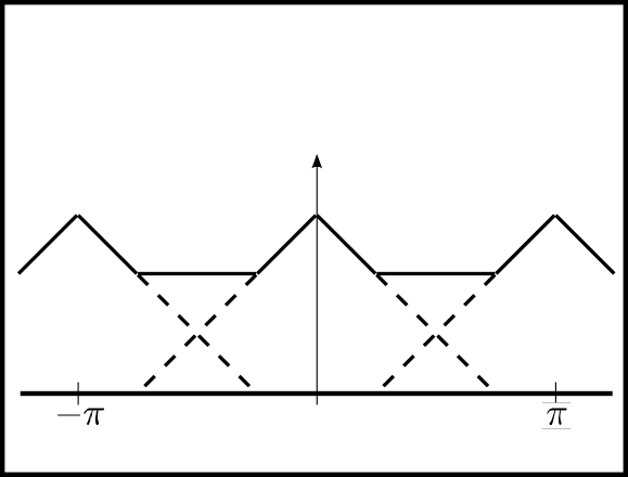
Refer to caption
(a) x𝑥x
Refer to caption
(b) xmsubscript𝑥𝑚x_{m}
Refer to caption
(c) xssubscript𝑥𝑠x_{s}
Refer to caption
(d) x^^𝑥\hat{x}
Refer to caption
(e) x^msubscript^𝑥𝑚\hat{x}_{m}
Refer to caption
(f) x^ssubscript^𝑥𝑠\hat{x}_{s}
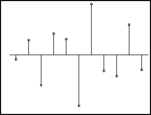
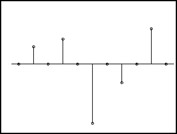
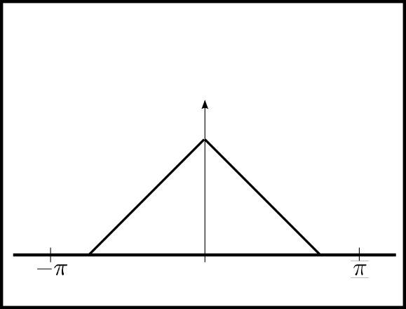
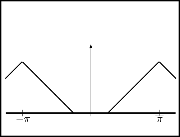
Figure 1: Pictorial illustrations of modulation and sampling in both the time (a-c) and frequency (d-f) domains.

Throughout, let x2()𝑥superscript2x\in\ell^{2}(\mathbb{Z}) be a real-valued sequence indexed by n𝑛n\in\mathbb{Z}. Subsampling is the operation of replacing every odd-numbered element of x𝑥x by zero, and hence the subsampled sequence xssubscript𝑥𝑠x_{s} is defined element-wise as

xs[n]subscript𝑥𝑠delimited-[]𝑛\displaystyle x_{s}[n] :={x[n]if n even,0if n odd.assignabsentcases𝑥delimited-[]𝑛if n even,0if n odd.\displaystyle:=\begin{cases}x[n]&\text{if $n$ even,}\\ 0&\text{if $n$ odd.}\end{cases}

(Note that this is distinct from downsampling, a dilation of the index set of x𝑥x to yield x[2n]𝑥delimited-[]2𝑛x[2n], such that odd-numbered samples are “dropped” and only even-numbered ones retained.) Equivalently, xs[n]subscript𝑥𝑠delimited-[]𝑛x_{s}[n] is an arithmetic average of x[n]𝑥delimited-[]𝑛x[n] and its frequency-modulated version xm[n]:=(1)nx[n].assignsubscript𝑥𝑚delimited-[]𝑛superscript1𝑛𝑥delimited-[]𝑛.x_{m}[n]:=(-1)^{n}x[n]\text{.}:

xs[n]=12(x[n]+xm[n]).subscript𝑥𝑠delimited-[]𝑛12𝑥delimited-[]𝑛subscript𝑥𝑚delimited-[]𝑛.\displaystyle x_{s}[n]=\frac{1}{2}\left(x[n]+x_{m}[n]\right)\text{.}

Figures 1(a)-(c) serve as a reminder to illustrate how samples in x𝑥x and xmsubscript𝑥𝑚x_{m} with opposite signs cancel out to yield xssubscript𝑥𝑠x_{s}; we shall frequently refer back to them later.

Let x^^𝑥\hat{x} denote the discrete-time Fourier transform of x𝑥x, with ω/2π𝜔2𝜋\omega\in\mathbb{R}/2\pi its corresponding normalized angular frequency. Then it follows that x^m(ω)=x^(ωπ)subscript^𝑥𝑚𝜔^𝑥𝜔𝜋\hat{x}_{m}(\omega)=\hat{x}(\omega-\pi) and

x^s(ω)subscript^𝑥𝑠𝜔\displaystyle\hat{x}_{s}(\omega) =12[x^(ω)+x^(ωπ)].absent12delimited-[]^𝑥𝜔^𝑥𝜔𝜋.\displaystyle=\frac{1}{2}\Big{[}\hat{x}(\omega)+\hat{x}(\omega-\pi)\Big{]}\text{.} (1)

Here we see that when the bandwidth of x𝑥x—i.e., the support of x^^𝑥\hat{x}—is sufficiently large, x^(ω)^𝑥𝜔\hat{x}(\omega) and x^m(ω)subscript^𝑥𝑚𝜔\hat{x}_{m}(\omega) are indistinguishable in x^s(ω)subscript^𝑥𝑠𝜔\hat{x}_{s}(\omega); as shown in Figures 1(d)-(g), their supports overlap in the Fourier domain. This phenomenon is called aliasing; in the absence of additional information, aliased portions of x𝑥x cannot be recovered from x^s(ω)subscript^𝑥𝑠𝜔\hat{x}_{s}(\omega) alone.

Refer to caption
(a) One-level filterbank structure
Refer to caption
(b) One-level complementary filterbank structure
Figure 2: One-level filterbank (a) and its complementary structure (b). Diagram (a) represents analysis and synthesis filters {g0,g1}subscript𝑔0subscript𝑔1\{g_{0},g_{1}\} and {h0,h1}subscript0subscript1\{h_{0},h_{1}\}, respectively, as well as filterbank coefficient sets {v0x,v1x}superscriptsubscript𝑣0𝑥superscriptsubscript𝑣1𝑥\{v_{0}^{x},v_{1}^{x}\} resulting from the action of the analysis convolution operator and subsequent downsampling on a sequence x𝑥x. Reversing the downsampling procedure and applying the synthesis filters yields a “reconstructed” sequence xrsubscript𝑥𝑟x_{r}. Diagram (b) represents filters g~i,h~isubscript~𝑔𝑖subscript~𝑖\tilde{g}_{i},\tilde{h}_{i} “complementary” to (a), obtained by swapping the roles of g𝑔g and hh, respectively, and then applying an affine transformation.

The Fourier transform is a fundamentally global operation; modulation and aliasing mix non-local information from the sequence x𝑥x. In contrast, a filterbank maps a sequence x𝑥x to some alternative representation by way of localized filterbank coefficients (“analysis”), and subsequently yields a linear reconstruction xrsubscript𝑥𝑟x_{r} (“synthesis”); well-known examples include short-time Fourier and wavelet representations. As the analysis operator acts linearly, we write its action as an inner product, calling it a filter when it is a convolution operator parameterized by translation along a sublattice of \mathbb{Z}, as is the case considered here. If this convolution operator is represented by the actions of a finite-length, real-valued sequences in 2()superscript2\ell^{2}(\mathbb{Z}), then we refer to a real-valued, finite-impulse-response analysis filter g𝑔g and corresponding synthesis filter hh. Figure 2(a) illustrates a basic filterbank structure, with two analysis filters {g0,g1}subscript𝑔0subscript𝑔1\{g_{0},g_{1}\} and two synthesis filters {h0,h1}subscript0subscript1\{h_{0},h_{1}\}. We denote by {v0x,v1x}superscriptsubscript𝑣0𝑥superscriptsubscript𝑣1𝑥\{v_{0}^{x},v_{1}^{x}\} the corresponding filterbank coefficient sequences, defined as follows.

Definition I.1 (Filterbank Coefficient Sequence)

We call vix2()subscriptsuperscript𝑣𝑥𝑖superscript2v^{x}_{i}\in\ell^{2}(\mathbb{Z}) a one-level filterbank coefficient sequence corresponding to x𝑥x if

vix[n]:=(gi[m]mx[m])[2n],assignsubscriptsuperscript𝑣𝑥𝑖delimited-[]𝑛subscript𝑚subscript𝑔𝑖delimited-[]𝑚𝑥delimited-[]𝑚delimited-[]2𝑛,\displaystyle v^{x}_{i}[n]:=\Big{(}g_{i}[m]\star_{m}x[m]\Big{)}[2n]\text{,} (2)

where the summation in the discrete convolution msubscript𝑚\star_{m} is performed over the index m𝑚m, and the subsequent notion of downsampling by two is reflected by the index set {2n:n}conditional-set2𝑛𝑛\{2n:n\in\mathbb{Z}\}.

This composition of convolution and dilation implies in turn that

v^ix(ω)=12[g^i(ω2)x^(ω2)+g^i(ω2π)x^(ω2π)],subscriptsuperscript^𝑣𝑥𝑖𝜔12delimited-[]subscript^𝑔𝑖𝜔2^𝑥𝜔2subscript^𝑔𝑖𝜔2𝜋^𝑥𝜔2𝜋,\displaystyle\hat{v}^{x}_{i}(\omega)=\frac{1}{2}\left[\hat{g}_{i}\left(\frac{\omega}{2}\right)\hat{x}\left(\frac{\omega}{2}\right)+\hat{g}_{i}\left(\frac{\omega}{2}-\pi\right)\hat{x}\left(\frac{\omega}{2}-\pi\right)\right]\text{,} (3)

and the set of transform coefficients {vix[n]}nsubscriptsubscriptsuperscript𝑣𝑥𝑖delimited-[]𝑛𝑛\{v^{x}_{i}[n]\}_{n\in\mathbb{Z}} is collectively referred to as the i𝑖ith filterbank subband. Typically g0subscript𝑔0g_{0} and h0subscript0h_{0} are smooth (i.e., low-pass) filters, while g1subscript𝑔1g_{1} and h1subscript1h_{1} have zero average. Thus, v0xsubscriptsuperscript𝑣𝑥0v^{x}_{0} provides a measure of local low-frequency energy concentration, while v1xsubscriptsuperscript𝑣𝑥1v^{x}_{1} captures local high-frequency energy, with temporal localization provided by the finite support of {gi,hi}i2subscriptsubscript𝑔𝑖subscript𝑖𝑖subscript2\{g_{i},h_{i}\}_{i\in\mathbb{Z}_{2}}. A filterbank’s joint time-frequency resolution can be fine-tuned by recursively nesting copies of the basic one-level transform structure illustrated in Figure 2(a), yielding the multi-level filterbank structures that we consider later in Section II-C.

Note that the Fourier representation of (3) implies the superposition of shifted copies of the resultant filtered spectra, which in general will give rise to aliasing of the type illustrated in Figure 1(f). It is thus natural to ask for conditions under which this aliasing will cancel—a prerequisite for the exact reconstruction of any input sequence x2()𝑥superscript2x\in\ell^{2}(\mathbb{Z}) from its filterbank coefficients, such that xr=xsubscript𝑥𝑟𝑥x_{r}=x in the diagram of Figure 2(a). To this end we arrive at the following well-known definition, which stems from global properties of the Fourier transform.

Definition I.2 (Perfect Reconstruction Filterbank)

A perfect reconstruction filterbank {gi,hi}i2subscriptsubscript𝑔𝑖subscript𝑖𝑖subscript2\{g_{i},h_{i}\}_{i\in\mathbb{Z}_{2}} admits for all x2()𝑥superscript2x\in\ell^{2}(\mathbb{Z}) the relation

x^(ω):=h^0(ω)v^x0(2ω)+h^1(ω)v^x1(2ω)=x^(ω).\displaystyle\hat{x}_{(}\omega):=\hat{h}_{0}(\omega)\hat{v}^{x}_{0}(2\omega)+\hat{h}_{1}(\omega)\hat{v}^{x}_{1}(2\omega)=\hat{x}(\omega)\text{.} (4)

Equivalently, as shown in Figure 2(a), we have for all n𝑛n\in\mathbb{Z} that

xr[2n]=subscript𝑥𝑟delimited-[]2𝑛absent\displaystyle x_{r}[2n]= (h0[2m]mv0x[m])[n]subscript𝑚subscript0delimited-[]2𝑚subscriptsuperscript𝑣𝑥0delimited-[]𝑚delimited-[]𝑛\displaystyle\Big{(}h_{0}[2m]\star_{m}v^{x}_{0}[m]\Big{)}[n]
+(h1[2m]mv1x[m])[n]=x[2n]subscript𝑚subscript1delimited-[]2𝑚subscriptsuperscript𝑣𝑥1delimited-[]𝑚delimited-[]𝑛𝑥delimited-[]2𝑛\displaystyle+\Big{(}h_{1}[2m]\star_{m}v^{x}_{1}[m]\Big{)}[n]=x[2n]
xr[2n+1]=subscript𝑥𝑟delimited-[]2𝑛1absent\displaystyle x_{r}[2n+1]= (h0[2m+1]mv0x[m])[n]subscript𝑚subscript0delimited-[]2𝑚1subscriptsuperscript𝑣𝑥0delimited-[]𝑚delimited-[]𝑛\displaystyle\Big{(}h_{0}[2m+1]\star_{m}v^{x}_{0}[m]\Big{)}[n]
+(h1[2m+1]mv1x[m])[n]=x[2n+1].subscript𝑚subscript1delimited-[]2𝑚1subscriptsuperscript𝑣𝑥1delimited-[]𝑚delimited-[]𝑛𝑥delimited-[]2𝑛1.\displaystyle+\Big{(}h_{1}[2m+1]\star_{m}v^{x}_{1}[m]\Big{)}[n]=x[2n+1]\text{.}

As described earlier, the sequences of operations corresponding to the forward transform step in (2) and the reconstruction step in (4) are commonly referred to as the analysis and synthesis filterbanks, respectively.

Remark I.1 (Haar Filterbank Transform)

Perhaps the most well-known example of a perfect reconstruction filterbank is given by the so-called Haar transform, which may be defined in terms of its z𝑧z-transform as:

ngi[n]zn=1+(1)iz,nhi[n]zn=12[(1)i+z1].subscript𝑛subscript𝑔𝑖delimited-[]𝑛superscript𝑧𝑛1superscript1𝑖𝑧,subscript𝑛subscript𝑖delimited-[]𝑛superscript𝑧𝑛12delimited-[]superscript1𝑖superscript𝑧1.\displaystyle\begin{split}\sum_{n}g_{i}[n]z^{-n}=&1+(-1)^{i}z\text{,}\\ \sum_{n}h_{i}[n]z^{-n}=&\frac{1}{2}\Big{[}(-1)^{i}+z^{-1}\Big{]}\text{.}\end{split} (5)

Note that g0subscript𝑔0g_{0} and g1subscript𝑔1g_{1} in (5) amount to the sum and difference of neighboring samples, respectively, and it is clear that the original sequence x[n]𝑥delimited-[]𝑛x[n] is easily recoverable from the corresponding sequences of filterbank coefficients.

Important and well-known results associated with Definition I.2 established the following (see, e.g., [1]) .

Property I.1 (Alias Cancellation Equivalence)

The set {gi,hi}i2subscriptsubscript𝑔𝑖subscript𝑖𝑖subscript2\{g_{i},h_{i}\}_{i\in\mathbb{Z}_{2}} is a perfect reconstruction filterbank if and only if

2=g^0(ω)h^0(ω)2subscript^𝑔0𝜔subscript^0𝜔\displaystyle 2=\hat{g}_{0}(\omega)\hat{h}_{0}(\omega) +g^1(ω)h^1(ω)subscript^𝑔1𝜔subscript^1𝜔\displaystyle+\hat{g}_{1}(\omega)\hat{h}_{1}(\omega) (6)
0=g^0(ω)h^0(ωπ)0subscript^𝑔0𝜔subscript^0𝜔𝜋\displaystyle 0=\hat{g}_{0}(\omega)\hat{h}_{0}(\omega-\pi) +g^1(ω)h^1(ωπ)subscript^𝑔1𝜔subscript^1𝜔𝜋\displaystyle+\hat{g}_{1}(\omega)\hat{h}_{1}(\omega-\pi) (7)
Property I.2 (Analysis-Synthesis Symmetry)

If finite-impulse-response filters {gi,hi}i2subscriptsubscript𝑔𝑖subscript𝑖𝑖subscript2\{g_{i},h_{i}\}_{i\in\mathbb{Z}_{2}} comprise a perfect reconstruction filterbank, then there exist a{0}𝑎0a\in\mathbb{R}\setminus\{0\} and b𝑏b\in\mathbb{Z} such that

g^i(ω)subscript^𝑔𝑖𝜔\displaystyle\hat{g}_{i}(\omega) =(1)1iaej(2b+1)ωh^1i(ωπ).absentsuperscript11𝑖𝑎superscript𝑒𝑗2𝑏1𝜔subscript^1𝑖𝜔𝜋.\displaystyle=(-1)^{1-i}ae^{j(2b+1)\omega}\hat{h}_{1-i}(\omega-\pi)\text{.}
Remark I.2

The condition of (7) in Property I.1 guarantees that the aliased components in v0xsubscriptsuperscript𝑣𝑥0v^{x}_{0} and v1xsubscriptsuperscript𝑣𝑥1v^{x}_{1} cancel, so the impulse response of the overall filterbank structure in Figure 2(a) is equal to one-half of the expression of (6); i.e., everywhere constant and equal to unity. Property I.2 makes explicit the fact that an analysis filterbank uniquely defines its corresponding synthesis filterbank. These properties serve as the foundation for the reverse-order subband filterbank structure that we introduce in Section II below.

I-B Motivating Example for Filterbank “Rewiring”

The preceding section has served to introduce the basic notions of filterbank theory that we shall employ here. Before continuing, it is instructive to consider a simple motivating example based on the simplest case of the Haar filterbank transform. In essence, we will see that “rewiring” filterbank diagrams such as those in Figure 3 can be related to the actions of convolution, modulation, and downsampling operators. In subsequent sections we develop these properties formally, and show how they yield new insights into important practical problems.

To begin, consider the symmetric Hadamard matrix

𝚽=[1111]𝚽matrix1111\bm{\Phi}=\begin{bmatrix}1&1\\ 1&-1\end{bmatrix}

which maps two-dimensional vectors to the corresponding sums and difference of their components, and thus serves to define the (unnormalized) one-level Haar filterbank. Note that 𝚽1=12𝚽superscript𝚽112𝚽\bm{\Phi}^{-1}=\frac{1}{2}\bm{\Phi}, and consider two systems of linear equations in 𝚽𝚽\bm{\Phi} that will serve to illustrate the concepts of reverse-order and convolution subband structure:

[qr]=matrix𝑞𝑟absent\displaystyle\begin{bmatrix}q\\ r\end{bmatrix}= 𝚽[ab],[st]=𝚽[cd].𝚽matrix𝑎𝑏matrix𝑠𝑡𝚽matrix𝑐𝑑.\displaystyle\bm{\Phi}\begin{bmatrix}a\\ b\end{bmatrix},\quad\begin{bmatrix}s\\ t\end{bmatrix}=\bm{\Phi}\begin{bmatrix}c\\ d\end{bmatrix}\text{.}
Example I.1 (Reverse-Ordering and Subsampling)

Consider the first system of equations above, and suppose that we replace b𝑏b with b𝑏-b, yielding a “modulated” version of [a,b]Tsuperscript𝑎𝑏𝑇[a,b]^{T}. We then observe that the Haar transform of [a,b]Tsuperscript𝑎𝑏𝑇[a,-b]^{T} results in a reverse-ordering of q𝑞q and r𝑟r, which play the roles of low-pass and high-pass components, respectively:

[1111][ab]=matrix1111matrix𝑎𝑏absent\displaystyle\begin{bmatrix}1&1\\ 1&-1\end{bmatrix}\begin{bmatrix}a\\ -b\end{bmatrix}= 12[1111][1111][qr]=[rq].12matrix1111matrix1111matrix𝑞𝑟matrix𝑟𝑞.\displaystyle\frac{1}{2}\begin{bmatrix}1&1\\ 1&-1\end{bmatrix}\begin{bmatrix}1&1\\ -1&1\end{bmatrix}\begin{bmatrix}q\\ r\end{bmatrix}=\begin{bmatrix}r\\ q\end{bmatrix}\text{.}

Since summing [a,b]Tsuperscript𝑎𝑏𝑇[a,b]^{T} and its modulated version corresponds to subsampling, we next compute the Haar transform of [a,0]Tsuperscript𝑎0𝑇[a,0]^{T}, and observe that this results in an arithmetic averaging of q𝑞q and r𝑟r:

[1111][a0]=matrix1111matrix𝑎0absent\displaystyle\begin{bmatrix}1&1\\ 1&-1\end{bmatrix}\begin{bmatrix}a\\ 0\end{bmatrix}= 12[1111]([ab]+[ab])=12[q+rq+r].12matrix1111matrix𝑎𝑏matrix𝑎𝑏12matrix𝑞𝑟𝑞𝑟.\displaystyle\frac{1}{2}\begin{bmatrix}1&1\\ 1&-1\end{bmatrix}\left(\begin{bmatrix}a\\ b\end{bmatrix}+\begin{bmatrix}a\\ -b\end{bmatrix}\right)=\frac{1}{2}\begin{bmatrix}q+r\\ q+r\end{bmatrix}\text{.}

We see from this simple example that the “swapping” and the “combining” of low-pass and high-pass components are reminiscent of modulation and aliasing in the traditional Fourier sense, as illustrated respectively in Figures 1(e) and 1(f).

Example I.2 (Convolution and Pointwise Multiplication)

Now consider the element-wise product of the vectors [a,b]Tsuperscript𝑎𝑏𝑇[a,b]^{T} and [c,d]Tsuperscript𝑐𝑑𝑇[c,d]^{T}. The Haar transform of this product [ac,bd]Tsuperscript𝑎𝑐𝑏𝑑𝑇[ac,bd]^{T} is:

[1111][acbd]=matrix1111matrix𝑎𝑐𝑏𝑑absent\displaystyle\begin{bmatrix}1&1\\ 1&-1\end{bmatrix}\begin{bmatrix}ac\\ bd\end{bmatrix}= 14[1111][(q+r)(s+t)(qr)(st)]14matrix1111matrix𝑞𝑟𝑠𝑡𝑞𝑟𝑠𝑡\displaystyle\frac{1}{4}\begin{bmatrix}1&1\\ 1&-1\end{bmatrix}\begin{bmatrix}(q+r)(s+t)\\ (q-r)(s-t)\end{bmatrix}
=\displaystyle= 14[(q+r)(s+t)+(qr)(st)(q+r)(s+t)(qr)(st)]14matrix𝑞𝑟𝑠𝑡𝑞𝑟𝑠𝑡𝑞𝑟𝑠𝑡𝑞𝑟𝑠𝑡\displaystyle\frac{1}{4}\begin{bmatrix}(q+r)(s+t)+(q-r)(s-t)\\ (q+r)(s+t)-(q-r)(s-t)\end{bmatrix}
=\displaystyle= 12[qs+rtqt+sr].12matrix𝑞𝑠𝑟𝑡𝑞𝑡𝑠𝑟.\displaystyle\frac{1}{2}\begin{bmatrix}qs+rt\\ qt+sr\end{bmatrix}\text{.}

The symmetry of qs+rt𝑞𝑠𝑟𝑡qs+rt and qt+sr𝑞𝑡𝑠𝑟qt+sr suggests a kind of cyclic convolution of [q,r]Tsuperscript𝑞𝑟𝑇[q,r]^{T} and [s,t]Tsuperscript𝑠𝑡𝑇[s,t]^{T}. In fact, we will see in Section III that our filterbank rewiring techniques recover precisely this notion of group structure, in direct analogy to global Fourier analysis. In Section IV, these ideas will reappear in the context of analysis of signals subject to multiplicative noise corruption.

II Reverse-Order Subband Structure and Localized Aliasing

Having introduced the necessary definitions and given two brief examples, we now begin our technical development of filterbank “rewiring.” Bearing in mind the examples considered above, we introduce in Section II-A below the notion of complementary filterbanks, and then employ them to obtain the following results in Section II-B: the reverse-ordering of subband structure that results from modulation, and localized aliasing that stems from averaging the low- and high-frequency filterbank coefficients. In Section II-C we extend these results to the setting of multi-level filterbanks.

II-A Complementary Filterbanks

Definition II.1

(Complementary Filterbanks and Filterbank Coefficients): Let {gi,hi}i2subscriptsubscript𝑔𝑖subscript𝑖𝑖subscript2\{g_{i},h_{i}\}_{i\in\mathbb{Z}_{2}} be a perfect reconstruction filterbank. Then we define the complementary filterbank {g~i,h~i}i2subscriptsubscript~𝑔𝑖subscript~𝑖𝑖subscript2\{\tilde{g}_{i},\tilde{h}_{i}\}_{i\in\mathbb{Z}_{2}} as follows:

g~i[n]:=assignsubscript~𝑔𝑖delimited-[]𝑛absent\displaystyle\tilde{g}_{i}[n]:= ahi[n+(2b+1)]𝑎subscript𝑖delimited-[]𝑛2𝑏1\displaystyle ah_{i}[n+(2b+1)]
h~i[n]:=assignsubscript~𝑖delimited-[]𝑛absent\displaystyle\tilde{h}_{i}[n]:= a1gi[n(2b+1)],superscript𝑎1subscript𝑔𝑖delimited-[]𝑛2𝑏1,\displaystyle a^{-1}g_{i}[n-(2b+1)]\text{,}

where a𝑎a and b𝑏b are chosen to satisfy Property I.2 of perfect reconstruction filterbank, and we call wix[n]superscriptsubscript𝑤𝑖𝑥delimited-[]𝑛w_{i}^{x}[n] a one-level complementary filterbank coefficient corresponding to a sequence x𝑥x if

wix[n]subscriptsuperscript𝑤𝑥𝑖delimited-[]𝑛\displaystyle w^{x}_{i}[n] :=(g~i[m]mx[m])[2n].assignabsentsubscript𝑚subscript~𝑔𝑖delimited-[]𝑚𝑥delimited-[]𝑚delimited-[]2𝑛.\displaystyle:=\Big{(}\tilde{g}_{i}[m]\star_{m}x[m]\Big{)}[2n]\text{.}

The following important property of complementary filterbanks follows directly from Properties I.1 and I.2 of perfect reconstruction filterbanks.

Proposition II.1 (Complementarity & Perfect Reconstruction)

If the set {gi,hi}i2subscriptsubscript𝑔𝑖subscript𝑖𝑖subscript2\{g_{i},h_{i}\}_{i\in\mathbb{Z}_{2}} is a perfect reconstruction filterbank, then so is {g~i,h~i}i2subscriptsubscript~𝑔𝑖subscript~𝑖𝑖subscript2\{\tilde{g}_{i},\tilde{h}_{i}\}_{i\in\mathbb{Z}_{2}}.

Proof:

Appealing to Property I.2, we see that Fourier transforms of g~isubscript~𝑔𝑖\tilde{g}_{i} and h~isubscript~𝑖\tilde{h}_{i} respectively yield

g~^i(ω)=aej(2b+1)ωh^i(ω)h~^i(ω)=a1ej(2b+1)ωg^i(ω).subscript^~𝑔𝑖𝜔𝑎superscript𝑒𝑗2𝑏1𝜔subscript^𝑖𝜔subscript^~𝑖𝜔superscript𝑎1superscript𝑒𝑗2𝑏1𝜔subscript^𝑔𝑖𝜔.\displaystyle\begin{split}\hat{\tilde{g}}_{i}(\omega)=&ae^{j(2b+1)\omega}\hat{h}_{i}(\omega)\\ \hat{\tilde{h}}_{i}(\omega)=&a^{-1}e^{-j(2b+1)\omega}\hat{g}_{i}(\omega)\text{.}\end{split} (8)

By substitution, we verify that (6) and (7) hold for {g~i,h~i}i2subscriptsubscript~𝑔𝑖subscript~𝑖𝑖subscript2\{\tilde{g}_{i},\tilde{h}_{i}\}_{i\in\mathbb{Z}_{2}}:

g~^0(ω)h~^0(ω)+g~^1(ω)h~^1(ω)subscript^~𝑔0𝜔subscript^~0𝜔subscript^~𝑔1𝜔subscript^~1𝜔\displaystyle\hat{\tilde{g}}_{0}(\omega)\hat{\tilde{h}}_{0}(\omega)+\hat{\tilde{g}}_{1}(\omega)\hat{\tilde{h}}_{1}(\omega)
=(aej(2b+1)ωh^0(ω))(a1ej(2b+1)g^0(ω))absent𝑎superscript𝑒𝑗2𝑏1𝜔subscript^0𝜔superscript𝑎1superscript𝑒𝑗2𝑏1subscript^𝑔0𝜔\displaystyle\quad=\Big{(}ae^{j(2b+1)\omega}\hat{h}_{0}(\omega)\Big{)}\Big{(}a^{-1}e^{-j(2b+1)}\hat{g}_{0}(\omega)\Big{)}
+(aej(2b+1)ωh^1(ω))(a1ej(2b+1)g^1(ω))=2𝑎superscript𝑒𝑗2𝑏1𝜔subscript^1𝜔superscript𝑎1superscript𝑒𝑗2𝑏1subscript^𝑔1𝜔2\displaystyle\quad\quad+\Big{(}ae^{j(2b+1)\omega}\hat{h}_{1}(\omega)\Big{)}\Big{(}a^{-1}e^{-j(2b+1)}\hat{g}_{1}(\omega)\Big{)}=2
g~^0(ω)h~^0(ωπ)+g~^1(ω)h~^1(ωπ)subscript^~𝑔0𝜔subscript^~0𝜔𝜋subscript^~𝑔1𝜔subscript^~1𝜔𝜋\displaystyle\hat{\tilde{g}}_{0}(\omega)\hat{\tilde{h}}_{0}(\omega-\pi)+\hat{\tilde{g}}_{1}(\omega)\hat{\tilde{h}}_{1}(\omega-\pi)
=(aej(2b+1)ωh^0(ω))(a1ej(2b+1)g^0(ωπ))absent𝑎superscript𝑒𝑗2𝑏1𝜔subscript^0𝜔superscript𝑎1superscript𝑒𝑗2𝑏1subscript^𝑔0𝜔𝜋\displaystyle\quad=\Big{(}ae^{j(2b+1)\omega}\hat{h}_{0}(\omega)\Big{)}\Big{(}a^{-1}e^{-j(2b+1)}\hat{g}_{0}(\omega-\pi)\Big{)}
+(aej(2b+1)ωh^1(ω))(a1ej(2b+1)g^1(ωπ))=0.𝑎superscript𝑒𝑗2𝑏1𝜔subscript^1𝜔superscript𝑎1superscript𝑒𝑗2𝑏1subscript^𝑔1𝜔𝜋0.\displaystyle\quad\quad+\Big{(}ae^{j(2b+1)\omega}\hat{h}_{1}(\omega)\Big{)}\Big{(}a^{-1}e^{-j(2b+1)}\hat{g}_{1}(\omega-\pi)\Big{)}=0\text{.}

Hence by Property I.1, the set {g~i,h~i}i2subscriptsubscript~𝑔𝑖subscript~𝑖𝑖subscript2\{\tilde{g}_{i},\tilde{h}_{i}\}_{i\in\mathbb{Z}_{2}} comprises a perfect reconstruction filterbank. ∎

Figure 2(b) illustrates this complementary filterbank structure, along with the corresponding complementary coefficients wixsubscriptsuperscript𝑤𝑥𝑖w^{x}_{i}. It is natural to ask if a filterbank can be its own complement, and to this end we have the following.

Definition II.2 (Self-Complementary Filterbank)

We call a filterbank {gi,hi}i2subscriptsubscript𝑔𝑖subscript𝑖𝑖subscript2\{g_{i},h_{i}\}_{i\in\mathbb{Z}_{2}} self-complementary if

vix[n]=(1)1iwix[n].subscriptsuperscript𝑣𝑥𝑖delimited-[]𝑛superscript11𝑖subscriptsuperscript𝑤𝑥𝑖delimited-[]𝑛.\displaystyle v^{x}_{i}[n]=(-1)^{1-i}w^{x}_{i}[n]\text{.} (9)

Returning now to Remark I.1, we note the following.

Proposition II.2 (Self-Complementarity of Haar Filterbank)

The Haar filterbank is self-complementary.

Proof:

It follows from (5) that the Haar filterbank satisfies the following symmetry:

g^i(ω)=(1)iej(2b+1)ωg^i(ω),subscript^𝑔𝑖𝜔superscript1𝑖superscript𝑒𝑗2𝑏1𝜔superscriptsubscript^𝑔𝑖𝜔,\displaystyle\hat{g}_{i}(\omega)=(-1)^{i}e^{j(2b+1)\omega}\hat{g}_{i}^{*}(\omega)\text{,}

with a=12𝑎12a=\frac{1}{2} and b=1𝑏1b=-1. Applying Property I.2 of perfect reconstruction filterbanks in turn yields

(1)iej(2b+1)ωg^i(ω)=superscript1𝑖superscript𝑒𝑗2𝑏1𝜔superscriptsubscript^𝑔𝑖𝜔absent\displaystyle(-1)^{i}e^{j(2b+1)\omega}\hat{g}_{i}^{*}(\omega)= (1)1iaej(2b+1)ωh^1i(ωπ)superscript11𝑖𝑎superscript𝑒𝑗2𝑏1𝜔subscript^1𝑖𝜔𝜋\displaystyle(-1)^{1-i}ae^{j(2b+1)\omega}\hat{h}_{1-i}(\omega-\pi)
g^i(ω)=superscriptsubscript^𝑔𝑖𝜔absent\displaystyle\hat{g}_{i}^{*}(\omega)= ah^1i(ωπ).𝑎subscript^1𝑖𝜔𝜋.\displaystyle-a\hat{h}_{1-i}(\omega-\pi)\text{.} (10)

The well-known identity g^i(ω)=(1)iej(2b+1)ωg^1i(ωπ)subscript^𝑔𝑖𝜔superscript1𝑖superscript𝑒𝑗2𝑏1𝜔superscriptsubscript^𝑔1𝑖𝜔𝜋\hat{g}_{i}(\omega)=(-1)^{i}e^{j(2b+1)\omega}\hat{g}_{1-i}^{*}(\omega-\pi) of Smith and Barnwell [13] applies; and upon substituting this into (II-A), we obtain the desired result:

g^i(ω)=subscript^𝑔𝑖𝜔absent\displaystyle\hat{g}_{i}(\omega)= (1)iej(2b+1)ω(ah^i(ω))superscript1𝑖superscript𝑒𝑗2𝑏1𝜔𝑎subscript^𝑖𝜔\displaystyle(-1)^{i}e^{j(2b+1)\omega}(-a\hat{h}_{i}(\omega))
=\displaystyle= (1)1ig~^i(ω).superscript11𝑖subscript^~𝑔𝑖𝜔.\displaystyle(-1)^{1-i}\hat{\tilde{g}}_{i}(\omega)\text{.}

As we show below, complementary filterbanks play a key role in the reverse-ordering of subband structure induced by modulation.

II-B Reverse-Order Subband Structure

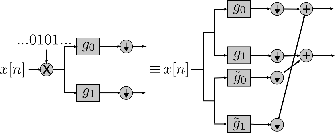
Figure 3 illustrates the reversal of subband ordering that results when x𝑥x is modulated by π𝜋\pi to yield xmsubscript𝑥𝑚x_{m}: the low-frequency filterbank coefficient for the modulated signal (v0xm[n]subscriptsuperscript𝑣subscript𝑥𝑚0delimited-[]𝑛v^{x_{m}}_{0}[n]) behaves like the high-frequency complementary filterbank coefficient for the original signal (w1x[n]subscriptsuperscript𝑤𝑥1delimited-[]𝑛w^{x}_{1}[n]), and vice-versa. As may be seen by comparing Figure 3 with Figure 1, this filterbank subband “role-reversal” is consistent with the Fourier interpretation of modulation by π𝜋\pi; in both cases, the low- and high-frequency components are swapped, modulo-2π2𝜋2\pi. We formalize this notion as follows:

Theorem 1 (Reverse-Order Subband Structure (ROSS))

If the set {gi,hi}i2subscriptsubscript𝑔𝑖subscript𝑖𝑖subscript2\{g_{i},h_{i}\}_{i\in\mathbb{Z}_{2}} is a perfect reconstruction filterbank, then

vixm[n]=(1)iw1ix[n].subscriptsuperscript𝑣subscript𝑥𝑚𝑖delimited-[]𝑛superscript1𝑖subscriptsuperscript𝑤𝑥1𝑖delimited-[]𝑛.\displaystyle v^{x_{m}}_{i}[n]=(-1)^{i}w^{x}_{1-i}[n]\text{.} (11)
Proof:

Modulation of x𝑥x by π𝜋\pi implies that we have that

v^ixm(ω)subscriptsuperscript^𝑣subscript𝑥𝑚𝑖𝜔\displaystyle\hat{v}^{x_{m}}_{i}(\omega) =12[g^i(ω2)x^m(ω2)+g^i(ω2π)x^m(ω2π)]absent12delimited-[]subscript^𝑔𝑖𝜔2subscript^𝑥𝑚𝜔2subscript^𝑔𝑖𝜔2𝜋subscript^𝑥𝑚𝜔2𝜋\displaystyle=\frac{1}{2}\left[\hat{g}_{i}\left(\frac{\omega}{2}\right)\hat{x}_{m}\left(\frac{\omega}{2}\right)+\hat{g}_{i}\left(\frac{\omega}{2}-\pi\right)\hat{x}_{m}\left(\frac{\omega}{2}-\pi\right)\right]
=12[g^i(ω2)x^(ω2π)+g^i(ω2π)x^(ω2)].absent12delimited-[]subscript^𝑔𝑖𝜔2^𝑥𝜔2𝜋subscript^𝑔𝑖𝜔2𝜋^𝑥𝜔2.\displaystyle=\frac{1}{2}\left[\hat{g}_{i}\left(\frac{\omega}{2}\right)\hat{x}\left(\frac{\omega}{2}-\pi\right)+\hat{g}_{i}\left(\frac{\omega}{2}-\pi\right)\hat{x}\left(\frac{\omega}{2}\right)\right]\text{.}

By Property I.2 of perfect reconstruction filterbanks and Definition II.1,

g^i(ω)=(1)1iaej(2b+1)ωh^1i(ωπ)subscript^𝑔𝑖𝜔superscript11𝑖𝑎superscript𝑒𝑗2𝑏1𝜔subscript^1𝑖𝜔𝜋\displaystyle\hat{g}_{i}(\omega)=(-1)^{1-i}ae^{j(2b+1)\omega}\hat{h}_{1-i}(\omega-\pi)
=(1)ig~^1i(ωπ)absentsuperscript1𝑖subscript^~𝑔1𝑖𝜔𝜋\displaystyle\quad=(-1)^{i}\hat{\tilde{g}}_{1-i}(\omega-\pi)
v^ixm(ω)subscriptsuperscript^𝑣subscript𝑥𝑚𝑖𝜔\displaystyle\hat{v}^{x_{m}}_{i}(\omega)
=(1)i2[g~^1i(ω2)x^(ω2)+g~^1i(ω2π)x^(ω2π)]absentsuperscript1𝑖2delimited-[]subscript^~𝑔1𝑖𝜔2^𝑥𝜔2subscript^~𝑔1𝑖𝜔2𝜋^𝑥𝜔2𝜋\displaystyle\quad=\frac{(-1)^{i}}{2}\left[\hat{\tilde{g}}_{1-i}\left(\frac{\omega}{2}\right)\hat{x}\left(\frac{\omega}{2}\right)+\hat{\tilde{g}}_{1-i}\left(\frac{\omega}{2}-\pi\right)\hat{x}\left(\frac{\omega}{2}-\pi\right)\right]
=(1)iw^1ix(ω).absentsuperscript1𝑖subscriptsuperscript^𝑤𝑥1𝑖𝜔.\displaystyle\quad=(-1)^{i}\hat{w}^{x}_{1-i}(\omega)\text{.} (12)

Refer to caption
Figure 3: Illustration of Theorem 1, with the left side showing a modulated signal xm[n]subscript𝑥𝑚delimited-[]𝑛x_{m}[n] and the right side showing reverse-ordering of the complementary filterbank. The low- and high-frequency filterbank subbands for the modulated signal behave like the high- and low-frequency complementary filterbank subbands for the original signal, respectively.

Applying Property I.1 of perfect reconstruction filterbanks to (II-B) immediately yields the following important corollary.

Corollary II.1 (Modulation induced by ROSS)

Suppose the set {gi,hi}i2subscriptsubscript𝑔𝑖subscript𝑖𝑖subscript2\{g_{i},h_{i}\}_{i\in\mathbb{Z}_{2}} is a perfect reconstruction filterbank. Then

0=0absent\displaystyle 0= g~^1(ω)h^0(ω)g~^0(ω)h^1(ω),subscript^~𝑔1𝜔subscript^0𝜔subscript^~𝑔0𝜔subscript^1𝜔\displaystyle\hat{\tilde{g}}_{1}(\omega)\hat{h}_{0}(\omega)-\hat{\tilde{g}}_{0}(\omega)\hat{h}_{1}(\omega),
2=2absent\displaystyle 2= g~^1(ω)h^0(ωπ)g~^0(ω)h^1(ωπ).subscript^~𝑔1𝜔subscript^0𝜔𝜋subscript^~𝑔0𝜔subscript^1𝜔𝜋.\displaystyle\hat{\tilde{g}}_{1}(\omega)\hat{h}_{0}(\omega-\pi)-\hat{\tilde{g}}_{0}(\omega)\hat{h}_{1}(\omega-\pi)\text{.}
Refer to caption
Figure 4: Illustration of Corollary II.1: exchange of low- and high-frequency filterbank subbands results in modulation (compare to the standard complementary filterbank structure of Figure 2(b)).
Remark II.1 (Filterbank Interpretation of ROSS Modulation)

An intuitive interpretation of Corollary II.1 is that exchanging the low- and high-frequency filterbank subbands results in modulation. To see this, consider reconstruction of the complementary filterbank coefficients with reverse-order subbands, as illustrated in Figure 4:

x^r(ω)subscript^𝑥𝑟𝜔\displaystyle\hat{x}_{r}(\omega) =h^0(ω)w^1x(2ω)h^1(ω)w^0x(2ω)absentsubscript^0𝜔subscriptsuperscript^𝑤𝑥12𝜔subscript^1𝜔subscriptsuperscript^𝑤𝑥02𝜔\displaystyle=\hat{h}_{0}(\omega)\hat{w}^{x}_{1}(2\omega)-\hat{h}_{1}(\omega)\hat{w}^{x}_{0}(2\omega)
=12h^0(ω)[g~^1(ω)x^(ω)+g~^1(ωπ)x^(ωπ)]absent12subscript^0𝜔delimited-[]subscript^~𝑔1𝜔^𝑥𝜔subscript^~𝑔1𝜔𝜋^𝑥𝜔𝜋\displaystyle=\frac{1}{2}\hat{h}_{0}(\omega)\Big{[}\hat{\tilde{g}}_{1}(\omega)\hat{x}(\omega)+\hat{\tilde{g}}_{1}(\omega-\pi)\hat{x}(\omega-\pi)\Big{]}
12h^1(ω)[g~^0(ω)x^(ω)+g~^0(ωπ)x^(ωπ)]12subscript^1𝜔delimited-[]subscript^~𝑔0𝜔^𝑥𝜔subscript^~𝑔0𝜔𝜋^𝑥𝜔𝜋\displaystyle\quad-\frac{1}{2}\hat{h}_{1}(\omega)\Big{[}\hat{\tilde{g}}_{0}(\omega)\hat{x}(\omega)+\hat{\tilde{g}}_{0}(\omega-\pi)\hat{x}(\omega-\pi)\Big{]}
=12x^(ω)[h^0(ω)g~^1(ω)h^1(ω)g~^0(ω)]absent12^𝑥𝜔delimited-[]subscript^0𝜔subscript^~𝑔1𝜔subscript^1𝜔subscript^~𝑔0𝜔\displaystyle=\frac{1}{2}\hat{x}(\omega)\Big{[}\hat{h}_{0}(\omega)\hat{\tilde{g}}_{1}(\omega)-\hat{h}_{1}(\omega)\hat{\tilde{g}}_{0}(\omega)\Big{]}
+12x^(ωπ)[h^0(ω)g~^1(ωπ)h^1(ω)g~^0(ωπ)]12^𝑥𝜔𝜋delimited-[]subscript^0𝜔subscript^~𝑔1𝜔𝜋subscript^1𝜔subscript^~𝑔0𝜔𝜋\displaystyle\quad+\frac{1}{2}\hat{x}(\omega-\pi)\Big{[}\hat{h}_{0}(\omega)\hat{\tilde{g}}_{1}(\omega-\pi)-\hat{h}_{1}(\omega)\hat{\tilde{g}}_{0}(\omega-\pi)\Big{]}
=x^(ωπ).absent^𝑥𝜔𝜋.\displaystyle=\hat{x}(\omega-\pi)\text{.}

We also obtain a filterbank interpretation of the aliasing induced by subsampling, in analogy to the Fourier decomposition of (1). As shown in Figure 5, filterbank coefficients corresponding to the subsampled signal xs[n]subscript𝑥𝑠delimited-[]𝑛x_{s}[n] are arithmetic averages of low- and high-frequency coefficients corresponding to x[n]𝑥delimited-[]𝑛x[n], in analogy to the symmetry about π/2𝜋2\pi/2 visible in the Figure 1(f).

Refer to caption
Figure 5: Illustration of Corollary II.2, with the left side showing x[n]𝑥delimited-[]𝑛x[n] subject to subsampling and the right side showing the corresponding aliasing structure. Filterbank coefficients corresponding to the subsampled signal are arithmetic averages of complementary low- and high-frequency coefficients.
Corollary II.2 (Localized Aliasing)

If the set {gi,hi}i2subscriptsubscript𝑔𝑖subscript𝑖𝑖subscript2\{g_{i},h_{i}\}_{i\in\mathbb{Z}_{2}} is a perfect reconstruction filterbank, then by linearity and Theorem 1,

vixs[n]=12(vix[n]+(1)iw1ix[n]).subscriptsuperscript𝑣subscript𝑥𝑠𝑖delimited-[]𝑛12subscriptsuperscript𝑣𝑥𝑖delimited-[]𝑛superscript1𝑖subscriptsuperscript𝑤𝑥1𝑖delimited-[]𝑛.\displaystyle v^{x_{s}}_{i}[n]=\frac{1}{2}\Big{(}v^{x}_{i}[n]+(-1)^{i}w^{x}_{1-i}[n]\Big{)}\text{.}

Furthermore, this modulation implies the filterbank subband symmetry vixs[n]=(1)iw1ixs[n]subscriptsuperscript𝑣subscript𝑥𝑠𝑖delimited-[]𝑛superscript1𝑖subscriptsuperscript𝑤subscript𝑥𝑠1𝑖delimited-[]𝑛v^{x_{s}}_{i}[n]=(-1)^{i}w^{x_{s}}_{1-i}[n].

As can be seen in Figure 5, localized aliasing occurs when vix[n]subscriptsuperscript𝑣𝑥𝑖delimited-[]𝑛v^{x}_{i}[n] and w1ix[n]subscriptsuperscript𝑤𝑥1𝑖delimited-[]𝑛w^{x}_{1-i}[n] are both simultaneously nonzero and hence indistinguishable in vixs[n]subscriptsuperscript𝑣subscript𝑥𝑠𝑖delimited-[]𝑛v^{x_{s}}_{i}[n]. Unlike the global Fourier aliasing illustrated in Figure 1, however, this aliasing is confined to a temporally localized region that depends on the local regularity of x𝑥x.

II-C Extension to Multi-Level Setting

Multi-level filterbank analysis corresponds to a recursive application of convolution and downsampling operators to successive sets of filterbank coefficients. To index the corresponding subbands, we adopt binary vector notation for indices as follows. Let 𝒊=(iI-1,,i1,i0)T2I𝒊superscriptsubscript𝑖𝐼-1subscript𝑖1subscript𝑖0𝑇superscriptsubscript2𝐼\bm{i}=(i_{I\text{-}1},\dots,i_{1},i_{0})^{T}\in{\mathbb{Z}_{2}}^{I} and 𝒊=(iI-1,,i1,1i0)Tsuperscript𝒊superscriptsubscript𝑖𝐼-1subscript𝑖11subscript𝑖0𝑇\bm{i}^{\prime}=(i_{I\text{-}1},\dots,i_{1},1-i_{0})^{T}, and recalling vix[n]subscriptsuperscript𝑣𝑥𝑖delimited-[]𝑛v^{x}_{i}[n] and wix[n]subscriptsuperscript𝑤𝑥𝑖delimited-[]𝑛w^{x}_{i}[n] from Definitions I.1 and II.1, define the corresponding I𝐼I-level recursions:

v𝒊x[n]:=(giI-1mI-1((gi1[m1]m1(gi0[m0]m0x[m0])[2m1])[2m2])[2mI-1])[2n]assignsubscriptsuperscript𝑣𝑥𝒊delimited-[]𝑛subscriptsubscript𝑚𝐼-1subscript𝑔subscript𝑖𝐼-1subscriptsubscript𝑚1subscript𝑔subscript𝑖1delimited-[]subscript𝑚1subscriptsubscript𝑚0subscript𝑔subscript𝑖0delimited-[]subscript𝑚0𝑥delimited-[]subscript𝑚0delimited-[]2subscript𝑚1delimited-[]2subscript𝑚2delimited-[]2subscript𝑚𝐼-1delimited-[]2𝑛\displaystyle\begin{split}v^{x}_{\bm{i}}[n]:=&\Big{(}g_{i_{I\text{-}1}}\star_{m_{I\text{-}1}}\Big{(}\dots\Big{(}g_{i_{1}}[m_{1}]\star_{m_{1}}\Big{(}g_{i_{0}}[m_{0}]\\ &\star_{m_{0}}x[m_{0}]\Big{)}[2m_{1}]\Big{)}[2m_{2}]\dots\Big{)}[2m_{I\text{-}1}]\Big{)}[2n]\end{split} (13)
w𝒊x[n]:=(giI-1mI-1((gi1[m1]m1(g~i0[m0]m0x[m0])[2m1])[2m2])[2mI-1])[2n].assignsubscriptsuperscript𝑤𝑥𝒊delimited-[]𝑛subscriptsubscript𝑚𝐼-1subscript𝑔subscript𝑖𝐼-1subscriptsubscript𝑚1subscript𝑔subscript𝑖1delimited-[]subscript𝑚1subscriptsubscript𝑚0subscript~𝑔subscript𝑖0delimited-[]subscript𝑚0𝑥delimited-[]subscript𝑚0delimited-[]2subscript𝑚1delimited-[]2subscript𝑚2delimited-[]2subscript𝑚𝐼-1delimited-[]2𝑛.\displaystyle\begin{split}w^{x}_{\bm{i}}[n]:=&\Big{(}g_{i_{I\text{-}1}}\star_{m_{I\text{-}1}}\Big{(}\dots\Big{(}g_{i_{1}}[m_{1}]\star_{m_{1}}\Big{(}\tilde{g}_{i_{0}}[m_{0}]\\ &\star_{m_{0}}x[m_{0}]\Big{)}[2m_{1}]\Big{)}[2m_{2}]\dots\Big{)}[2m_{I\text{-}1}]\Big{)}[2n]\text{.}\end{split} (14)

Here ik2subscript𝑖𝑘subscript2i_{k}\in\mathbb{Z}_{2} indexes the analysis filters used in the k𝑘kth-level decomposition (i.e. g0subscript𝑔0g_{0} or g1subscript𝑔1g_{1}), and 𝒊superscript𝒊\bm{i}^{\prime} corresponds to a high (low) frequency subband when 𝒊𝒊\bm{i} is a low (high) frequency subband. Note here that the complementary filters g~0subscript~𝑔0\tilde{g}_{0} and g~1subscript~𝑔1\tilde{g}_{1} are used only in the 00th-level decomposition in (14). The corresponding perfect reconstruction extension of (4) to the case of an I𝐼I-level filterbank is

x^r(ω):=𝒊v^𝒊x(2Iω)k=0I1h^ik(2kω).assignsubscript^𝑥𝑟𝜔subscript𝒊subscriptsuperscript^𝑣𝑥𝒊superscript2𝐼𝜔superscriptsubscriptproduct𝑘0𝐼1subscript^subscript𝑖𝑘superscript2𝑘𝜔.\displaystyle\hat{x}_{r}(\omega):=\sum_{\bm{i}}\hat{v}^{x}_{\bm{i}}(2^{I}\omega)\prod_{k=0}^{I-1}\hat{h}_{i_{k}}(2^{k}\omega)\text{.} (15)

Then, in parallel to our earlier development, the results of Theorem 1 and Corollary II.2 extend to the multi-level setting as follows.

Theorem 2 (Multi-Level ROSS)

Suppose the set {gi,hi}i2subscriptsubscript𝑔𝑖subscript𝑖𝑖subscript2\{g_{i},h_{i}\}_{i\in\mathbb{Z}_{2}} is a perfect reconstruction filterbank, and let 𝐢2I𝐢superscriptsubscript2𝐼\bm{i}\in{\mathbb{Z}_{2}}^{I}. Then,

v𝒊xm=subscriptsuperscript𝑣subscript𝑥𝑚𝒊absent\displaystyle v^{x_{m}}_{\bm{i}}= (1)i0w𝒊x[n];superscript1subscript𝑖0subscriptsuperscript𝑤𝑥superscript𝒊delimited-[]𝑛\displaystyle(-1)^{i_{0}}w^{x}_{\bm{i}^{\prime}}[n];
v𝒊xs=subscriptsuperscript𝑣subscript𝑥𝑠𝒊absent\displaystyle v^{x_{s}}_{\bm{i}}= (1)i0w𝒊xs[n]=12(v𝒊x[n]+(1)i0w𝒊x[n]).superscript1subscript𝑖0subscriptsuperscript𝑤subscript𝑥𝑠superscript𝒊delimited-[]𝑛12subscriptsuperscript𝑣𝑥𝒊delimited-[]𝑛superscript1subscript𝑖0subscriptsuperscript𝑤𝑥superscript𝒊delimited-[]𝑛.\displaystyle(-1)^{i_{0}}w^{x_{s}}_{\bm{i}^{\prime}}[n]=\frac{1}{2}\Big{(}v^{x}_{\bm{i}}[n]+(-1)^{i_{0}}w^{x}_{\bm{i}^{\prime}}[n]\Big{)}\text{.}

Using the same example shown in Figure 1, Figure 6 illustrates this localized aliasing in the multi-level filterbank setting. Note that although the subsampled example signal is subject to aliasing in a global sense (Figure 1(f)), the corresponding v𝒊x[n]subscriptsuperscript𝑣𝑥𝒊delimited-[]𝑛v^{x}_{\bm{i}}[n] may be recovered from v𝒊xs[n]subscriptsuperscript𝑣subscript𝑥𝑠𝒊delimited-[]𝑛v^{x_{s}}_{\bm{i}}[n] whenever w𝒊x[n]=0subscriptsuperscript𝑤𝑥superscript𝒊delimited-[]𝑛0w^{x}_{\bm{i}^{\prime}}[n]=0. Theorem 2 simplifies when self-complimentarity is taken into account, illustrated also in Figure 7.

Corollary II.3 (Multi-Level Self-Complementary ROSS)

If the set {gi,hi}i2subscriptsubscript𝑔𝑖subscript𝑖𝑖subscript2\{g_{i},h_{i}\}_{i\in\mathbb{Z}_{2}} is a perfect reconstruction filterbank that is also self-complementary, then

v𝒊x[n]=subscriptsuperscript𝑣𝑥𝒊delimited-[]𝑛absent\displaystyle v^{x}_{\bm{i}}[n]= (1)1i0w𝒊x[n],superscript11subscript𝑖0subscriptsuperscript𝑤𝑥𝒊delimited-[]𝑛,\displaystyle(-1)^{1-i_{0}}w^{x}_{\bm{i}}[n]\text{,}
v𝒊xm[n]=subscriptsuperscript𝑣subscript𝑥𝑚𝒊delimited-[]𝑛absent\displaystyle v^{x_{m}}_{\bm{i}}[n]= v𝒊x[n];subscriptsuperscript𝑣𝑥superscript𝒊delimited-[]𝑛;\displaystyle v^{x}_{\bm{i}^{\prime}}[n]\text{;}
v𝒊xs[n]=subscriptsuperscript𝑣subscript𝑥𝑠𝒊delimited-[]𝑛absent\displaystyle v^{x_{s}}_{\bm{i}}[n]= 12(v𝒊x[n]+v𝒊xm[n])=12(v𝒊x[n]+v𝒊x[n]).12subscriptsuperscript𝑣𝑥𝒊delimited-[]𝑛subscriptsuperscript𝑣subscript𝑥𝑚𝒊delimited-[]𝑛12subscriptsuperscript𝑣𝑥𝒊delimited-[]𝑛subscriptsuperscript𝑣𝑥superscript𝒊delimited-[]𝑛.\displaystyle\frac{1}{2}\Big{(}v^{x}_{\bm{i}}[n]+v^{x_{m}}_{\bm{i}}[n]\Big{)}=\frac{1}{2}\Big{(}v^{x}_{\bm{i}}[n]+v^{x}_{\bm{i}^{\prime}}[n]\Big{)}\text{.}
Refer to caption
(a) v𝒊xsubscriptsuperscript𝑣𝑥𝒊v^{x}_{\bm{i}}
Refer to caption
(b) v𝒊xmsubscriptsuperscript𝑣subscript𝑥𝑚𝒊v^{x_{m}}_{\bm{i}}
Refer to caption
(c) v𝒊xssubscriptsuperscript𝑣subscript𝑥𝑠𝒊v^{x_{s}}_{\bm{i}}
Refer to caption
(d) w𝒊xsubscriptsuperscript𝑤𝑥𝒊w^{x}_{\bm{i}}
Figure 6: Pictorial illustration of localized aliasing in the 2-level filterbank domain, as indicated by Theorem 2. Parts (a-c) show filterbank coefficients sequences corresponding to Fig. 1(a-c), respectively, with (d) the complementary sequence corresponding to Fig. 1(a). From top to bottom, the ordering of the four subbands represented in each subfigure is 𝒊=(0,0),(1,0),(1,1),(0,1)𝒊00101101\bm{i}=(0,0),(1,0),(1,1),(0,1). “Rewiring” is evident in comparing (b) with (d), and v𝒊x[n]subscriptsuperscript𝑣𝑥𝒊delimited-[]𝑛v^{x}_{\bm{i}}[n] is exactly recoverable from v𝒊xs[n]subscriptsuperscript𝑣subscript𝑥𝑠𝒊delimited-[]𝑛v^{x_{s}}_{\bm{i}}[n] whenever w𝒊x[n]=0subscriptsuperscript𝑤𝑥superscript𝒊delimited-[]𝑛0w^{x}_{\bm{i}^{\prime}}[n]=0.
Refer to caption
Figure 7: Illustration of Corollary II.3. Filterbank coefficients corresponding to the subsampled signal are arithmetic averages of reverse-order coefficients. Localized aliasing thus occurs when v𝒊x[n]subscriptsuperscript𝑣𝑥𝒊delimited-[]𝑛v^{x}_{\bm{i}}[n] and w𝒊x[n]subscriptsuperscript𝑤𝑥superscript𝒊delimited-[]𝑛w^{x}_{\bm{i}^{\prime}}[n] are both supported simultaneously and hence indistinguishable in vixs[n]subscriptsuperscript𝑣subscript𝑥𝑠𝑖delimited-[]𝑛v^{x_{s}}_{i}[n].
Remark II.2 (Extension to Discrete Wavelet Transform)

The above results can easily be adapted to discrete wavelet transforms, which employ the same fundamental building blocks as perfect reconstruction filterbanks [1, 2]. As an example, the filterbank rewiring associated with the wavelet transform of a subsampled signal xs[n]subscript𝑥𝑠delimited-[]𝑛x_{s}[n] is illustrated in Figure 8; we leave the details as an easy exercise for the reader.

Refer to caption
Figure 8: An example of ROSS-based wavelet analysis, with the left side showing x[n]𝑥delimited-[]𝑛x[n] subject to subsampling, and the right side showing the corresponding aliasing structure.

III Subband Convolution Structure and Localized Modulation

In the previous section, we introduced and studied the reverse-ordering of subband structure induced by subsampling, for the case of general perfect reconstruction filterbanks. Furthermore, we saw that this structure simplified considerably when self-complimentarity was taken into account. In this section, we show that the symmetry of the Haar filterbank transform also affords a characterization of Fourier group duality and convolution. As a special case, we recover the multi-level ROSS structure of Corollary II.3, thereby linking the ROSS results of Section II and the subband convolution structure (SCS) we introduce below.

III-A Subband Convolution Structure

Recall the multi-level filterbank decomposition of (13), in which ik2subscript𝑖𝑘subscript2i_{k}\in{\mathbb{Z}_{2}} indexes pairs of analysis filters used for the k𝑘kth level decomposition. Below, we prove the duality of time-domain multiplication and subband convolution of filterbank coefficients in this context.

Theorem 3 (Subband Convolution)

Let v𝐢x,v𝐢ysubscriptsuperscript𝑣𝑥𝐢subscriptsuperscript𝑣𝑦𝐢v^{x}_{\bm{i}},v^{y}_{\bm{i}} be I𝐼I-level Haar filterbank coefficient sequences corresponding to x𝑥x and y𝑦y, respectively, with v𝐢xy[n]superscriptsubscript𝑣𝐢𝑥𝑦delimited-[]𝑛v_{\bm{i}}^{xy}[n] that of the element-wise product xy𝑥𝑦xy. Then, letting \circledast denote cyclic convolution, we have the relation

(v𝒋x𝒋v𝒋y)𝒊[n]:=12I𝒋v𝒊+𝒋x[n]v𝒋y[n]=v𝒊xy[n].assignsubscriptsubscript𝒋subscriptsuperscript𝑣𝑥𝒋subscriptsuperscript𝑣𝑦𝒋𝒊delimited-[]𝑛1superscript2𝐼subscript𝒋subscriptsuperscript𝑣𝑥𝒊𝒋delimited-[]𝑛subscriptsuperscript𝑣𝑦𝒋delimited-[]𝑛subscriptsuperscript𝑣𝑥𝑦𝒊delimited-[]𝑛.\displaystyle\Big{(}v^{x}_{\bm{j}}\circledast_{\bm{j}}v^{y}_{\bm{j}}\Big{)}_{\bm{i}}[n]:=\frac{1}{2^{I}}\sum_{\bm{j}}v^{x}_{\bm{i}+\bm{j}}[n]v^{y}_{\bm{j}}[n]=v^{xy}_{\bm{i}}[n]\text{.}
Proof:

By the Fourier representation of (15), the product x[n]y[n]𝑥delimited-[]𝑛𝑦delimited-[]𝑛x[n]\cdot y[n] can be analyzed as:

(xy)^(ω)=x^r(ω)ωy^r(ω)^𝑥𝑦𝜔subscript𝜔subscript^𝑥𝑟𝜔subscript^𝑦𝑟𝜔\displaystyle\widehat{(x\cdot y)}(\omega)=\hat{x}_{r}(\omega)\star_{\omega}\hat{y}_{r}(\omega)
=[𝒊v^𝒊x(2Iω)k=0I1h^ik(2kω)]ω[𝒋v^𝒋x(2Iω)k=0I1h^jk(2kω)]absentsubscript𝜔delimited-[]subscript𝒊subscriptsuperscript^𝑣𝑥𝒊superscript2𝐼𝜔superscriptsubscriptproduct𝑘0𝐼1subscript^subscript𝑖𝑘superscript2𝑘𝜔delimited-[]subscript𝒋subscriptsuperscript^𝑣𝑥𝒋superscript2𝐼𝜔superscriptsubscriptproduct𝑘0𝐼1subscript^subscript𝑗𝑘superscript2𝑘𝜔\displaystyle=\left[\sum_{\bm{i}}\hat{v}^{x}_{\bm{i}}(2^{I}\omega)\prod_{k=0}^{I-1}\hat{h}_{i_{k}}(2^{k}\omega)\right]\star_{\omega}\left[\sum_{\bm{j}}\hat{v}^{x}_{\bm{j}}(2^{I}\omega)\prod_{k=0}^{I-1}\hat{h}_{j_{k}}(2^{k}\omega)\right]
=𝒊𝒋ππv^𝒊x(2Iν)v^𝒋x(2I(ων))[k=0I1h^ik(2kν)h^jk(2k(ων))]dν.\displaystyle\begin{split}&=\sum_{\bm{i}}\sum_{\bm{j}}\int_{-\pi}^{\pi}\hat{v}^{x}_{\bm{i}}(2^{I}\nu)\hat{v}^{x}_{\bm{j}}\Big{(}2^{I}(\omega-\nu)\Big{)}\\ &\quad\quad\cdot\left[\prod_{k=0}^{I-1}\hat{h}_{i_{k}}(2^{k}\nu)\hat{h}_{j_{k}}\Big{(}2^{k}(\omega-\nu)\Big{)}\right]d\nu\text{.}\end{split} (16)

It follows from the definition of the Haar filterbank transform in (5) that

h^ik(2kν)h^jk(2k(ων))subscript^subscript𝑖𝑘superscript2𝑘𝜈subscript^subscript𝑗𝑘superscript2𝑘𝜔𝜈\displaystyle\hat{h}_{i_{k}}(2^{k}\nu)\hat{h}_{j_{k}}\Big{(}2^{k}(\omega-\nu)\Big{)}
=14[(1)ik+ej2kν][(1)jk+ej2k(ων)]absent14delimited-[]superscript1subscript𝑖𝑘superscript𝑒𝑗superscript2𝑘𝜈delimited-[]superscript1subscript𝑗𝑘superscript𝑒𝑗superscript2𝑘𝜔𝜈\displaystyle=\frac{1}{4}\left[(-1)^{i_{k}}+e^{-j2^{k}\nu}\right]\left[(-1)^{j_{k}}+e^{-j2^{k}(\omega-\nu)}\right]
=12[h^ik+jk(2kω)+(1)ikej2kνh^ik+jk(2k(ω2ν))].absent12delimited-[]subscript^subscript𝑖𝑘subscript𝑗𝑘superscript2𝑘𝜔superscript1subscript𝑖𝑘superscript𝑒𝑗superscript2𝑘𝜈subscript^subscript𝑖𝑘subscript𝑗𝑘superscript2𝑘𝜔2𝜈.\displaystyle=\frac{1}{2}\left[\hat{h}_{i_{k}+j_{k}}(2^{k}\omega)+(-1)^{i_{k}}e^{-j2^{k}\nu}\hat{h}_{i_{k}+j_{k}}\left(2^{k}(\omega-2\nu)\right)\right]\text{.}

Substituting this expression into (III-A) for k=0𝑘0k=0,

(xy)^(ω)=12𝒊𝒋ππv^𝒊x(2Iν)v^𝒋x^𝑥𝑦𝜔12subscript𝒊subscript𝒋superscriptsubscript𝜋𝜋subscriptsuperscript^𝑣𝑥𝒊superscript2𝐼𝜈subscriptsuperscript^𝑣𝑥𝒋\displaystyle\widehat{(x\cdot y)}(\omega)=\frac{1}{2}\sum_{\bm{i}}\sum_{\bm{j}}\int_{-\pi}^{\pi}\hat{v}^{x}_{\bm{i}}(2^{I}\nu)\hat{v}^{x}_{\bm{j}}
(2I(ων))[k=1I1h^ik(2kν)h^jk(2k(ων))]absentsuperscript2𝐼𝜔𝜈delimited-[]superscriptsubscriptproduct𝑘1𝐼1subscript^subscript𝑖𝑘superscript2𝑘𝜈subscript^subscript𝑗𝑘superscript2𝑘𝜔𝜈\displaystyle\quad\quad\cdot\Big{(}2^{I}(\omega-\nu)\Big{)}\left[\prod_{k=1}^{I-1}\hat{h}_{i_{k}}(2^{k}\nu)\hat{h}_{j_{k}}\Big{(}2^{k}(\omega-\nu)\Big{)}\right]
[h^i0+j0(ω)+(1)i0ejνh^i0+j0(ω2ν)]dνabsentdelimited-[]subscript^subscript𝑖0subscript𝑗0𝜔superscript1subscript𝑖0superscript𝑒𝑗𝜈subscript^subscript𝑖0subscript𝑗0𝜔2𝜈𝑑𝜈\displaystyle\quad\quad\cdot\left[\hat{h}_{i_{0}+j_{0}}(\omega)+(-1)^{i_{0}}e^{-j\nu}\hat{h}_{i_{0}+j_{0}}(\omega-2\nu)\right]d\nu
=12𝒊𝒋h^i0+j0(ω)ππv^𝒊x(2Iν)v^𝒋x(2I(ων))absent12subscript𝒊subscript𝒋subscript^subscript𝑖0subscript𝑗0𝜔superscriptsubscript𝜋𝜋subscriptsuperscript^𝑣𝑥𝒊superscript2𝐼𝜈subscriptsuperscript^𝑣𝑥𝒋superscript2𝐼𝜔𝜈\displaystyle\quad=\frac{1}{2}\sum_{\bm{i}}\sum_{\bm{j}}\hat{h}_{i_{0}+j_{0}}(\omega)\int_{-\pi}^{\pi}\hat{v}^{x}_{\bm{i}}(2^{I}\nu)\hat{v}^{x}_{\bm{j}}\Big{(}2^{I}(\omega-\nu)\Big{)}
[k=1I1h^ik(2kν)h^jk(2k(ων))]dν,absentdelimited-[]superscriptsubscriptproduct𝑘1𝐼1subscript^subscript𝑖𝑘superscript2𝑘𝜈subscript^subscript𝑗𝑘superscript2𝑘𝜔𝜈𝑑𝜈,\displaystyle\quad\quad\cdot\left[\prod_{k=1}^{I-1}\hat{h}_{i_{k}}(2^{k}\nu)\hat{h}_{j_{k}}\Big{(}2^{k}(\omega-\nu)\Big{)}\right]d\nu\text{,}

where we have used the fact that ππej2kνf^(ν)𝑑ν=0superscriptsubscript𝜋𝜋superscript𝑒𝑗superscript2𝑘𝜈^𝑓𝜈differential-d𝜈0\int_{-\pi}^{\pi}e^{-j2^{k}\nu}\hat{f}(\nu)d\nu=0 for all f^(ν)L(/2kπ)^𝑓𝜈𝐿superscript2𝑘𝜋\hat{f}(\nu)\in L(\mathbb{R}/2^{-k}\pi) whenever k0𝑘0k\geq 0, as ej(2kνπ)f^(ν2kπ)=ej2kνf^(ν)superscript𝑒𝑗superscript2𝑘𝜈𝜋^𝑓𝜈superscript2𝑘𝜋superscript𝑒𝑗superscript2𝑘𝜈^𝑓𝜈e^{-j(2^{k}\nu-\pi)}\hat{f}(\nu-2^{-k}\pi)=-e^{-j2^{k}\nu}\hat{f}(\nu). By recursion over k𝑘k, the above reduces to

(xy)^(ω)=12K𝒊𝒋[k=0K1h^ik+jk(2kω)]ππv^𝒊x(2Iν)v^𝒋x(2I(ων))[k=KI1h^ik(2kν)h^jk(2k(ων))]dν=12K+1𝒊𝒋[k=0Kh^ik+jk(2kω)]ππv^𝒊x(2Iν)v^𝒋x(2I(ων))[k=K+1I1h^ik(2kν)h^jk(2k(ων))]dν==12I𝒊𝒋[k=0I1h^ik+jk(2kω)][v^𝒊x(2Iω)ωv^𝒋y(2Iω)].^𝑥𝑦𝜔1superscript2𝐾subscript𝒊subscript𝒋delimited-[]superscriptsubscriptproduct𝑘0𝐾1subscript^subscript𝑖𝑘subscript𝑗𝑘superscript2𝑘𝜔superscriptsubscript𝜋𝜋subscriptsuperscript^𝑣𝑥𝒊superscript2𝐼𝜈subscriptsuperscript^𝑣𝑥𝒋superscript2𝐼𝜔𝜈delimited-[]superscriptsubscriptproduct𝑘𝐾𝐼1subscript^subscript𝑖𝑘superscript2𝑘𝜈subscript^subscript𝑗𝑘superscript2𝑘𝜔𝜈𝑑𝜈1superscript2𝐾1subscript𝒊subscript𝒋delimited-[]superscriptsubscriptproduct𝑘0𝐾subscript^subscript𝑖𝑘subscript𝑗𝑘superscript2𝑘𝜔superscriptsubscript𝜋𝜋subscriptsuperscript^𝑣𝑥𝒊superscript2𝐼𝜈subscriptsuperscript^𝑣𝑥𝒋superscript2𝐼𝜔𝜈delimited-[]superscriptsubscriptproduct𝑘𝐾1𝐼1subscript^subscript𝑖𝑘superscript2𝑘𝜈subscript^subscript𝑗𝑘superscript2𝑘𝜔𝜈𝑑𝜈1superscript2𝐼subscript𝒊subscript𝒋delimited-[]superscriptsubscriptproduct𝑘0𝐼1subscript^subscript𝑖𝑘subscript𝑗𝑘superscript2𝑘𝜔delimited-[]subscript𝜔subscriptsuperscript^𝑣𝑥𝒊superscript2𝐼𝜔subscriptsuperscript^𝑣𝑦𝒋superscript2𝐼𝜔.\displaystyle\begin{split}\widehat{(x\cdot y)}(\omega)=&\frac{1}{2^{K}}\sum_{\bm{i}}\sum_{\bm{j}}\left[\prod_{k=0}^{K-1}\hat{h}_{i_{k}+j_{k}}(2^{k}\omega)\right]\\ &\cdot\int_{-\pi}^{\pi}\hat{v}^{x}_{\bm{i}}(2^{I}\nu)\hat{v}^{x}_{\bm{j}}\Big{(}2^{I}(\omega-\nu)\Big{)}\\ &\cdot\left[\prod_{k=K}^{I-1}\hat{h}_{i_{k}}(2^{k}\nu)\hat{h}_{j_{k}}\Big{(}2^{k}(\omega-\nu)\Big{)}\right]d\nu\\ =&\frac{1}{2^{K+1}}\sum_{\bm{i}}\sum_{\bm{j}}\left[\prod_{k=0}^{K}\hat{h}_{i_{k}+j_{k}}(2^{k}\omega)\right]\\ &\cdot\int_{-\pi}^{\pi}\hat{v}^{x}_{\bm{i}}(2^{I}\nu)\hat{v}^{x}_{\bm{j}}\Big{(}2^{I}(\omega-\nu)\Big{)}\\ &\cdot\left[\prod_{k=K+1}^{I-1}\hat{h}_{i_{k}}(2^{k}\nu)\hat{h}_{j_{k}}\Big{(}2^{k}(\omega-\nu)\Big{)}\right]d\nu\\ =\dots=&\frac{1}{2^{I}}\sum_{\bm{i}}\sum_{\bm{j}}\left[\prod_{k=0}^{I-1}\hat{h}_{i_{k}+j_{k}}(2^{k}\omega)\right]\\ &\cdot\left[\hat{v}^{x}_{\bm{i}}(2^{I}\omega)\star_{\omega}\hat{v}^{y}_{\bm{j}}(2^{I}\omega)\right]\text{.}\end{split} (17)

Note that (17) takes the form of a multi-level inverse filterbank transform, as per (15). As the Haar filterbank transform is one-to-one and onto, v𝒊xysuperscriptsubscript𝑣𝒊𝑥𝑦v_{\bm{i}}^{xy} is thus uniquely defined by

v^𝒊xy(ω)=12I𝒋[v^𝒊+𝒋x(ω)ωv^𝒋y(ω)],subscriptsuperscript^𝑣𝑥𝑦𝒊𝜔1superscript2𝐼subscript𝒋delimited-[]subscript𝜔subscriptsuperscript^𝑣𝑥𝒊𝒋𝜔subscriptsuperscript^𝑣𝑦𝒋𝜔,\displaystyle\hat{v}^{xy}_{\bm{i}}(\omega)=\frac{1}{2^{I}}\sum_{\bm{j}}\left[\hat{v}^{x}_{\bm{i}+\bm{j}}(\omega)\star_{\omega}\hat{v}^{y}_{\bm{j}}(\omega)\right]\text{,}

which agrees with the claim of the theorem. ∎

Figure 9 illustrates the corresponding “rewiring” of filterbank subbands, in which v𝒊x[n]subscriptsuperscript𝑣𝑥𝒊delimited-[]𝑛v^{x}_{\bm{i}}[n] and v𝒊y[n]subscriptsuperscript𝑣𝑦𝒊delimited-[]𝑛v^{y}_{\bm{i}}[n] are coupled together to yield v0xy[n]subscriptsuperscript𝑣𝑥𝑦0delimited-[]𝑛v^{xy}_{0}[n], and v𝒊x[n]subscriptsuperscript𝑣𝑥superscript𝒊delimited-[]𝑛v^{x}_{\bm{i}^{\prime}}[n] and v𝒊y[n]subscriptsuperscript𝑣𝑦𝒊delimited-[]𝑛v^{y}_{\bm{i}}[n] are combined to produce v1xysubscriptsuperscript𝑣𝑥𝑦1v^{xy}_{1}.

Refer to caption
Figure 9: Illustration of Theorem 3, showing the correspondence between time-domain multiplication and “logical convolution” of filterbank subbands.
Remark III.1 (Logical Convolution)

By restricting x𝑥x and y𝑦y be finite-dimensional, we recover the so-called logical convolution theorem [14] as a special case of Theorem 3. This is easily seen by considering an order-2Isuperscript2𝐼2^{I} Walsh sequence ϕ𝐢2Isubscriptitalic-ϕ𝐢superscriptsuperscript2𝐼\vec{\phi}_{\bm{i}}\in\mathbb{R}^{2^{I}} and its Abelian structure:

diag(ϕ𝒊)ϕ𝒋=ϕ𝒊+𝒋,𝒊,𝒋{2}I.formulae-sequencediagsubscriptitalic-ϕ𝒊subscriptitalic-ϕ𝒋subscriptitalic-ϕ𝒊𝒋𝒊𝒋superscriptsubscript2𝐼.\displaystyle\text{diag}(\vec{\phi}_{\bm{i}})\vec{\phi}_{\bm{j}}=\vec{\phi}_{\bm{i}+\bm{j}},\quad\bm{i},\bm{j}\in\{\mathbb{Z}_{2}\}^{I}\text{.} (18)

Orthogonality of the Walsh basis sets implies that any x2I𝑥superscriptsuperscript2𝐼\vec{x}\in\mathbb{R}^{2^{I}} can be expanded in terms of its Walsh-Hadamard coefficients ϕ𝐢,x=ϕ𝐢Txsubscriptitalic-ϕ𝐢𝑥superscriptsubscriptitalic-ϕ𝐢𝑇𝑥\Big{\langle}\vec{\phi}_{\bm{i}},\vec{x}\Big{\rangle}=\vec{\phi}_{\bm{i}}^{T}\vec{x} as x=2I𝐣ϕ𝐣,xϕ𝐣𝑥superscript2𝐼subscript𝐣subscriptitalic-ϕ𝐣𝑥subscriptitalic-ϕ𝐣\vec{x}=2^{-I}\sum_{\bm{j}}\Big{\langle}\vec{\phi}_{\bm{j}},\vec{x}\Big{\rangle}\vec{\phi}_{\bm{j}}, and hence the group homomorphism of (18) yields the desired relation for all x,y2I𝑥𝑦superscriptsuperscript2𝐼\vec{x},\vec{y}\in\mathbb{R}^{2^{I}}:

ϕ𝒊,diag(x)y=subscriptitalic-ϕ𝒊diag𝑥𝑦absent\displaystyle\Big{\langle}\vec{\phi}_{\bm{i}},\text{diag}(\vec{x})\vec{y}\Big{\rangle}= 122I𝒋,𝒋ϕ𝒋,xϕ𝒋,yϕ𝒊,diag(ϕ𝒋)ϕ𝒋1superscript22𝐼subscript𝒋superscript𝒋subscriptitalic-ϕ𝒋𝑥subscriptitalic-ϕsuperscript𝒋𝑦subscriptitalic-ϕ𝒊diagsubscriptitalic-ϕ𝒋subscriptitalic-ϕsuperscript𝒋\displaystyle\frac{1}{2^{2I}}\sum_{\bm{j},\bm{j}^{\prime}}\Big{\langle}\vec{\phi}_{\bm{j}},\vec{x}\Big{\rangle}\Big{\langle}\vec{\phi}_{\bm{j}^{\prime}},\vec{y}\Big{\rangle}\Big{\langle}\vec{\phi}_{\bm{i}},\text{diag}(\vec{\phi}_{\bm{j}})\vec{\phi}_{\bm{j}^{\prime}}\Big{\rangle}
=\displaystyle= 12I𝒋ϕ𝒋,xϕ𝒊+𝒋,y.1superscript2𝐼subscript𝒋subscriptitalic-ϕ𝒋𝑥subscriptitalic-ϕ𝒊𝒋𝑦.\displaystyle\frac{1}{2^{I}}\sum_{\bm{j}}\Big{\langle}\vec{\phi}_{\bm{j}},\vec{x}\Big{\rangle}\Big{\langle}\vec{\phi}_{\bm{i}+\bm{j}},\vec{y}\Big{\rangle}\text{.}

III-B Localized Modulation and Connection to Reverse-Ordered Subband Structure

We conclude this section by interpreting the result of Theorem 3 in terms of amplitude modulation and sampling.

Remark III.2 (Multi-Level ROSS for Haar Filterbank Transform)

Suppose that we set v(0,,0,0)y[n]=v(0,,0,1)y[n]=2I1subscriptsuperscript𝑣𝑦000delimited-[]𝑛subscriptsuperscript𝑣𝑦001delimited-[]𝑛superscript2𝐼1v^{y}_{(0,\dots,0,0)}[n]=v^{y}_{(0,\dots,0,1)}[n]=2^{I-1} for all n𝑛n, and v𝐢y[n]=0subscriptsuperscript𝑣𝑦𝐢delimited-[]𝑛0v^{y}_{\bm{i}}[n]=0 otherwise, thus yielding a Dirac comb. Then Theorem 3 agrees precisely with Corollary II.3:

(v𝒋x𝒋v𝒋y)𝒊[n]=subscriptsubscript𝒋subscriptsuperscript𝑣𝑥𝒋subscriptsuperscript𝑣𝑦𝒋𝒊delimited-[]𝑛absent\displaystyle\Big{(}v^{x}_{\bm{j}}\circledast_{\bm{j}}v^{y}_{\bm{j}}\Big{)}_{\bm{i}}[n]= 12(v𝒊x[n]+v𝒊x[n]).12subscriptsuperscript𝑣𝑥𝒊delimited-[]𝑛subscriptsuperscript𝑣𝑥superscript𝒊delimited-[]𝑛.\displaystyle\frac{1}{2}\Big{(}v^{x}_{\bm{i}}[n]+v^{x}_{\bm{i}^{\prime}}[n]\Big{)}\text{.}
Remark III.3 (Generalized Subsampling)

More generally, suppose y[n]{0,1}𝑦delimited-[]𝑛01y[n]\in\{0,1\} is a sampling mask of any kind. Then it may be seen from Figure 9 that the subsampled signal x[n]y[n]𝑥delimited-[]𝑛𝑦delimited-[]𝑛x[n]y[n] is aliased if v0x[n]v0y[n]subscriptsuperscript𝑣𝑥0delimited-[]𝑛subscriptsuperscript𝑣𝑦0delimited-[]𝑛v^{x}_{0}[n]v^{y}_{0}[n] and v1x[n]v1y[n]subscriptsuperscript𝑣𝑥1delimited-[]𝑛subscriptsuperscript𝑣𝑦1delimited-[]𝑛v^{x}_{1}[n]v^{y}_{1}[n] (or, v0x[n]v1y[n]subscriptsuperscript𝑣𝑥0delimited-[]𝑛subscriptsuperscript𝑣𝑦1delimited-[]𝑛v^{x}_{0}[n]v^{y}_{1}[n] and v0x[n]v1y[n]subscriptsuperscript𝑣𝑥0delimited-[]𝑛subscriptsuperscript𝑣𝑦1delimited-[]𝑛v^{x}_{0}[n]v^{y}_{1}[n]) are simultaneously supported.

Remark III.4 (Localized Modulation)

Consider Figure 9 again and suppose at time n=0𝑛0n=0, we have that v0y[n]=0subscriptsuperscript𝑣𝑦0delimited-[]𝑛0v^{y}_{0}[n]=0 and v1y[n]=1subscriptsuperscript𝑣𝑦1delimited-[]𝑛1v^{y}_{1}[n]=1. Then v0x[n]subscriptsuperscript𝑣𝑥0delimited-[]𝑛v^{x}_{0}[n] is “modulated” to v1xy[n]subscriptsuperscript𝑣𝑥𝑦1delimited-[]𝑛v^{xy}_{1}[n]. This is similar to Fourier amplitude modulation, in which case the energy of the modulated signal is concentrated around a chosen carrier frequency; however, a representation based on Theorem 3 is amenable to temporally local processing. For example, suppose at time n=1𝑛1n=1, we take v0y[n]=1subscriptsuperscript𝑣𝑦0delimited-[]𝑛1v^{y}_{0}[n]=1 and v1y[n]=0subscriptsuperscript𝑣𝑦1delimited-[]𝑛0v^{y}_{1}[n]=0; then v0x[n]subscriptsuperscript𝑣𝑥0delimited-[]𝑛v^{x}_{0}[n] is mapped to v0xy[n]subscriptsuperscript𝑣𝑥𝑦0delimited-[]𝑛v^{xy}_{0}[n] instead of v1xy[n]subscriptsuperscript𝑣𝑥𝑦1delimited-[]𝑛v^{xy}_{1}[n]. In other words, this filterbank interpretation of localized modulation—illustrated in Figure 10—is ideal for tracking modulation when the “carrier” y[n]𝑦delimited-[]𝑛y[n] is allowed to change over time.

Formally, we are concerned with characterizing a sum z[n]=kxk[n]yk[n]𝑧delimited-[]𝑛subscript𝑘subscript𝑥𝑘delimited-[]𝑛subscript𝑦𝑘delimited-[]𝑛z[n]=\sum_{k}x_{k}[n]y_{k}[n] of modulated sequences xksubscript𝑥𝑘x_{k}. When the “envelope function” yk[n]subscript𝑦𝑘delimited-[]𝑛y_{k}[n] is chosen carefully, then it follows from Theorem 3 that these signals are recoverable.

Proposition III.1 (Localized Amplitude Modulation)

Suppose yk[n]subscript𝑦𝑘delimited-[]𝑛y_{k}[n] is defined by a sequence of index values 𝐣k{2}Isubscript𝐣𝑘superscriptsubscript2𝐼\bm{j}_{k}\in\{\mathbb{Z}_{2}\}^{I} and Haar filterbank coefficients: v𝐢yk[n]=δ(𝐢,𝐣k[n])subscriptsuperscript𝑣subscript𝑦𝑘𝐢delimited-[]𝑛𝛿𝐢subscript𝐣𝑘delimited-[]𝑛v^{y_{k}}_{\bm{i}}[n]=\delta(\bm{i},\bm{j}_{k}[n]). Then xk[n]subscript𝑥𝑘delimited-[]𝑛x_{k}[n] is recoverable from z[n]=kxk[n]yk[n]𝑧delimited-[]𝑛subscript𝑘subscript𝑥𝑘delimited-[]𝑛subscript𝑦𝑘delimited-[]𝑛z[n]=\sum_{k}x_{k}[n]y_{k}[n] when the supports of v𝐢+𝐣k[n]xk[n]subscriptsuperscript𝑣subscript𝑥𝑘𝐢subscript𝐣𝑘delimited-[]𝑛delimited-[]𝑛v^{x_{k}}_{\bm{i}+\bm{j}_{k}[n]}[n] are mutually exclusive for all 𝐢𝐢\bm{i} and k𝑘k.

Proof:

By the subband convolution result of Theorem 3,

v𝒊z[n]=subscriptsuperscript𝑣𝑧𝒊delimited-[]𝑛absent\displaystyle v^{z}_{\bm{i}}[n]= kv𝒊xkyk[n]=k(v𝒋xk𝒋v𝒋yk)𝒊[n]=kv𝒊+𝒋k[n]xk[n]subscript𝑘subscriptsuperscript𝑣subscript𝑥𝑘subscript𝑦𝑘𝒊delimited-[]𝑛subscript𝑘subscriptsubscript𝒋subscriptsuperscript𝑣subscript𝑥𝑘𝒋subscriptsuperscript𝑣subscript𝑦𝑘𝒋𝒊delimited-[]𝑛subscript𝑘subscriptsuperscript𝑣subscript𝑥𝑘𝒊subscript𝒋𝑘delimited-[]𝑛delimited-[]𝑛\displaystyle\sum_{k}v^{x_{k}y_{k}}_{\bm{i}}[n]=\sum_{k}\Big{(}v^{x_{k}}_{\bm{j}}\circledast_{\bm{j}}v^{y_{k}}_{\bm{j}}\Big{)}_{\bm{i}}[n]=\sum_{k}v^{x_{k}}_{\bm{i}+\bm{j}_{k}[n]}[n]

However, by the assumed mutual exclusivity of the supports of v𝒊+𝒋k[n]xk[n]subscriptsuperscript𝑣subscript𝑥𝑘𝒊subscript𝒋𝑘delimited-[]𝑛delimited-[]𝑛v^{x_{k}}_{\bm{i}+\bm{j}_{k}[n]}[n], it follows that

v𝒊z[n]={v𝒊+𝒋k[n]xk[n]if there exists k with nonzero v𝒊+𝒋k[n]xk0otherwise,subscriptsuperscript𝑣𝑧𝒊delimited-[]𝑛casessubscriptsuperscript𝑣subscript𝑥𝑘𝒊subscript𝒋𝑘delimited-[]𝑛delimited-[]𝑛if there exists k with nonzero v𝒊+𝒋k[n]xk0otherwise,\displaystyle v^{z}_{\bm{i}}[n]=\left\{\begin{array}[]{ll}v^{x_{k}}_{\bm{i}+\bm{j}_{k}[n]}[n]&\text{if there exists $k$ with nonzero $v^{x_{k}}_{\bm{i}+\bm{j}_{k}[n]}$}\\ 0&\text{otherwise,}\end{array}\right.

and thus we conclude that v𝒊xk[n]=v𝒊+𝒋k[n]z[n]subscriptsuperscript𝑣subscript𝑥𝑘𝒊delimited-[]𝑛subscriptsuperscript𝑣𝑧𝒊subscript𝒋𝑘delimited-[]𝑛delimited-[]𝑛v^{x_{k}}_{\bm{i}}[n]=v^{z}_{\bm{i}+\bm{j}_{k}[n]}[n] whenever v𝒊vk[n]subscriptsuperscript𝑣subscript𝑣𝑘𝒊delimited-[]𝑛v^{v_{k}}_{\bm{i}}[n] is nonzero. ∎

Refer to caption
(a) v𝒊xsubscriptsuperscript𝑣𝑥𝒊v^{x}_{\bm{i}}
Refer to caption
(b) v𝒊ysubscriptsuperscript𝑣𝑦𝒊v^{y}_{\bm{i}}
Refer to caption
(c) v𝒊xysubscriptsuperscript𝑣𝑥𝑦𝒊v^{xy}_{\bm{i}}
Figure 10: Pictorial illustration of localized modulation in 2-level filterbank domain. Time-domain multiplication of x𝑥x and y𝑦y, represented by their filterbank coefficients in (a) and (b), results in subband convolution, shown in (c); “rewiring” is evident in comparing (a) and (c). Exact recovery of v𝒊x[n]subscriptsuperscript𝑣𝑥𝒊delimited-[]𝑛v^{x}_{\bm{i}}[n] from v𝒊xy[n]subscriptsuperscript𝑣𝑥𝑦𝒊delimited-[]𝑛v^{xy}_{\bm{i}}[n] is possible when the supports of v𝒊+𝒋x[n]subscriptsuperscript𝑣𝑥𝒊𝒋delimited-[]𝑛v^{x}_{\bm{i}+\bm{j}}[n] are mutually exclusive for all 𝒊𝒊\bm{i} and 𝒋𝒋\bm{j} corresponding to nonzero v𝒊x[n]subscriptsuperscript𝑣𝑥𝒊delimited-[]𝑛v^{x}_{\bm{i}}[n] and v𝒋y[n]subscriptsuperscript𝑣𝑦𝒋delimited-[]𝑛v^{y}_{\bm{j}}[n].

IV Discussion: Implications for Signal Analysis

The preceding two sections have explored properties of reverse-order and convolution subband structure (ROSS and SCS) in filterbanks, and shown their relation to the concepts of localized aliasing and modulation. We now discuss the practical implications of these results for signal analysis, and provide two brief demonstrations that “rewiring” filterbank diagrams in the manner of ROSS and SCS can enable new solutions to problems involving subsampled data corrupted by additive or multiplicative noise. As many scientific and engineering applications give rise to inverse problems involving subsampled and/or noisy data, and since filterbanks are the tool of choice for many signal and image processing tasks, it is natural to analyze the data likelihoods resulting from these problems directly in the filterbank coefficient domain.

IV-A Filterbank-Domain Likelihoods via ROSS and SCS

While data likelihoods often do not admit straightforward closed-form expressions through traditional filterbank analysis, the ROSS and SCS concepts provide a new way to characterize signals subject to aliasing or signal-dependent noise effects directly in the filterbank coefficient domain, by virtue of the associated filterbank rewiring techniques. The expression of filterbank data likelihoods is key to solving signal reconstruction and enhancement problems in this context; as signal acquisition models, these likelihoods may be coupled with regularization terms that encourages parsimony as a means of signal modeling, reflected through prior probability densities on filterbank coefficients, or equivalently through terms that explicitly penalize complexity. To this end, the following two corollaries show how explicit likelihood formulations follow directly from application of the ROSS and SCS concepts introduced earlier.

Corollary IV.1 (Noisy, Subsampled Data Likelihood)

Fix x2()𝑥superscript2x\in\ell^{2}(\mathbb{Z}) as the signal of interest, and let ξ𝜉\xi comprise samples of white Gaussian noise of variance σ2superscript𝜎2\sigma^{2}. Suppose then that we observe subsampled, noisy data y=xs+ξs𝑦subscript𝑥𝑠subscript𝜉𝑠y=x_{s}+\xi_{s} and subsequently apply a unitary filterbank transform; then it follows from the localized aliasing relation of Theorem 2 that the analysis filterbank coefficients of y𝑦y satisfy

v𝒊y[n]=subscriptsuperscript𝑣𝑦𝒊delimited-[]𝑛absent\displaystyle v^{y}_{\bm{i}}[n]= v𝒊x[n]+(1)i0w𝒊x[n]2+v𝒊ξ[n]+(1)i0w𝒊ξ[n]2,subscriptsuperscript𝑣𝑥𝒊delimited-[]𝑛superscript1subscript𝑖0subscriptsuperscript𝑤𝑥superscript𝒊delimited-[]𝑛2subscriptsuperscript𝑣𝜉𝒊delimited-[]𝑛superscript1subscript𝑖0subscriptsuperscript𝑤𝜉superscript𝒊delimited-[]𝑛2,\displaystyle\frac{v^{x}_{\bm{i}}[n]+(-1)^{i_{0}}w^{x}_{\bm{i}^{\prime}}[n]}{2}+\frac{v^{\xi}_{\bm{i}}[n]+(-1)^{i_{0}}w^{\xi}_{\bm{i}^{\prime}}[n]}{2}\text{,}

and hence each admits a Normal likelihood with mean (v𝐢x[n]+(1)i0w𝐢x[n])/2subscriptsuperscript𝑣𝑥𝐢delimited-[]𝑛superscript1subscript𝑖0subscriptsuperscript𝑤𝑥superscript𝐢delimited-[]𝑛2\big{(}v^{x}_{\bm{i}}[n]+(-1)^{i_{0}}w^{x}_{\bm{i}^{\prime}}[n]\big{)}/2 and variance σ2/2superscript𝜎22\sigma^{2}/2.

Corollary IV.2 (Multiplicative Noise Data Likelihood)

Suppose instead that the observation model y[n]=x[n]+x[n]ξ[n]𝑦delimited-[]𝑛𝑥delimited-[]𝑛𝑥delimited-[]𝑛𝜉delimited-[]𝑛y[n]=x[n]+x[n]\xi[n] is in force. Then the subband convolution structure of Theorem 3 implies the filterbank coefficient relation

v𝒊y[n]=subscriptsuperscript𝑣𝑦𝒊delimited-[]𝑛absent\displaystyle v^{y}_{\bm{i}}[n]= v𝒊x[n]+(v𝒋x[n]𝒋v𝒋ξ[n])𝒊,subscriptsuperscript𝑣𝑥𝒊delimited-[]𝑛subscriptsubscript𝒋subscriptsuperscript𝑣𝑥𝒋delimited-[]𝑛subscriptsuperscript𝑣𝜉𝒋delimited-[]𝑛𝒊,\displaystyle v^{x}_{\bm{i}}[n]+\Big{(}v^{x}_{\bm{j}}[n]\circledast_{\bm{j}}v^{\xi}_{\bm{j}}[n]\Big{)}_{\bm{i}}\text{,}

and hence the likelihood form of v𝐢y[n]subscriptsuperscript𝑣𝑦𝐢delimited-[]𝑛v^{y}_{\bm{i}}[n] is multivariate Normal with mean v𝐢x[n]subscriptsuperscript𝑣𝑥𝐢delimited-[]𝑛v^{x}_{\bm{i}}[n], where the covariance of v𝐢y[n]subscriptsuperscript𝑣𝑦𝐢delimited-[]𝑛v^{y}_{\bm{i}}[n] and v𝐣y[n]subscriptsuperscript𝑣𝑦𝐣delimited-[]𝑛v^{y}_{\bm{j}}[n] is given by σ2(v𝐤x𝐤v𝐤x)𝐢+𝐣superscript𝜎2subscriptsubscript𝐤subscriptsuperscript𝑣𝑥𝐤subscriptsuperscript𝑣𝑥𝐤𝐢𝐣\sigma^{2}(v^{x}_{\bm{k}}\circledast_{\bm{k}}v^{x}_{\bm{k}})_{\bm{i}+\bm{j}}.

IV-B Proof of Concept: Application to Image Interpolation and Denoising

The likelihood expressions of Corollaries IV.1 and IV.2 above extend straightforwardly to the case of separable two-dimensional filterbank transforms, which in turn are typically employed in imaging applications. Thus, to illustrate the practical applicability of these results, we now undertake two proof-of-concept experiments that are representative of problems frequently encountered in digital imaging, and for which our ROSS and SCS characterizations—in contrast to standard approaches—yield closed-form likelihood expressions for the corresponding filterbank coefficients.

The first of these—image interpolation in the presence of noise—is made difficult by the fact that low- and high-frequency filterbank subbands interact with one another as well as with the noise itself; the “rewiring” expression of Corollary IV.1 in turn provides a closed-form likelihood expression for the filterbank coefficients. In the second experiment, we consider the similarly difficult problem of mitigating multiplicative noise; in this case, Corollary IV.2 yields the corresponding likelihood.

As filterbank coefficients of images typically exhibit sparsity[15], one natural approach to utilize these likelihoods through a Bayesian framework, in which transform coefficients of the underlying image x𝑥x are modeled as random variables v𝒊X[n]superscriptsubscript𝑣𝒊𝑋delimited-[]𝑛v_{\bm{i}}^{X}[n] taking zero-mean, symmetric, and unimodal “heavy-tailed” distributions that exhibit super-Gaussian tail behavior[16, 17]. We assume such a prior distribution here, and evaluate posterior means numerically via Monte Carlo averages.

We follow typical practice in approximating the overall joint posterior distribution of all filterbank coefficients by a product of marginal distributions, where each marginal posterior is associated with a particular subband. In turn, the 2superscript2\ell^{2}-optimal estimator of filterbank coefficients v𝒊X[n]superscriptsubscript𝑣𝒊𝑋delimited-[]𝑛v_{\bm{i}}^{X}[n] corresponding to the 𝒊𝒊\bm{i}th subband given the corresponding data coefficients v𝒊y[n]superscriptsubscript𝑣𝒊𝑦delimited-[]𝑛v_{\bm{i}}^{y}[n] is given by

𝔼[v𝒊X|v𝒊y]=v𝒊xp(v𝒊y|v𝒊x)p(v𝒊x)𝑑v𝒊xp(v𝒊y);𝔼delimited-[]conditionalsubscriptsuperscript𝑣𝑋𝒊subscriptsuperscript𝑣𝑦𝒊subscriptsuperscript𝑣𝑥𝒊𝑝conditionalsubscriptsuperscript𝑣𝑦𝒊subscriptsuperscript𝑣𝑥𝒊𝑝subscriptsuperscript𝑣𝑥𝒊differential-dsubscriptsuperscript𝑣𝑥𝒊𝑝subscriptsuperscript𝑣𝑦𝒊;\displaystyle\mathbb{E}[v^{X}_{\bm{i}}|v^{y}_{\bm{i}}]=\frac{\int v^{x}_{\bm{i}}p(v^{y}_{\bm{i}}|v^{x}_{\bm{i}})p(v^{x}_{\bm{i}})dv^{x}_{\bm{i}}}{p(v^{y}_{\bm{i}})}\text{;} (19)

the corresponding synthesis filterbank in turn allows reconstruction of the estimated image.

We first consider a well-known 8-bit test image that has been artificially downsampled and degraded with additive white Gaussian noise of variance 400 to yield a signal-to-noise ratio (SNR) of 16.77 dB relative to xssubscript𝑥𝑠x_{s} (or 1.22 dB relative to x𝑥x), as shown in Figures 11(a) and 11(b). Figure 11(c) shows the corresponding image reconstruction, which retains much of sharpness of the image edges and textures while suppressing noise, resulting in an SNR gain of 3.81 dB. For purposes of comparison, Figure 11(d) shows the result of the recently proposed simultaneous interpolation and denoising method of [18], which yields an SNR gain of 3.55 dB; this reconstruction exhibits edges that are more strongly preserved, but at the expense of greater smoothing of image textures.

In our second experiment, we consider a synthetic aperture radar (SAR) image, available at www.sandia.gov/radar; as may be seen from Figure 12(a), such images suffer from the effects of multiplicative noise [19]. Figure 12(b) shows the enhanced image resulting from a “rewiring” approach, which exhibits reduced noise in smooth and textured regions, and avoids the introduction of artifacts. In contrast, Figure 12(c) illustrates the standard approach: application of a logarithmic transformation to the data, followed by an additive denoising technique (here the well-known method of [16]) and subsequent exponentiation of the result. Not only are Bayes optimality properties of [16] lost in the exponentiation transformation back to the pixel domain, but also substantial artifacts are seen to result from this standard approach.

Refer to caption
(a) Original test image
Refer to caption
(b) Subsampled, noisy test image
Refer to caption
(c) “Rewiring” reconstruction
Refer to caption
(d) Reconstruction via the method of [18]
Figure 11: Example of noisy image interpolation via the ROSS technique of Section II: The first row shows a full-resolution 8-bit test image (a), along with a subsampled version that has been degraded with additive white Gaussian noise of variance 400 (b). The bottom row shows a posterior mean reconstruction based on the filterbank-domain likelihood of Corollary IV.1 and a heavy-tailed prior distribution on filterbank coefficients (c), along with a reconstruction according to the recently proposed method of [18], shown for comparison (d).
Refer to caption
(a) SAR image showing “speckled noise”
Refer to caption
(b) “Rewiring” enhancement
Refer to caption
(c) Enhancement via the method of [16], applied after logarithmic transformation
Figure 12: Example of multiplicative noise mitigation via the SCS technique of Section III: Panel (a) shows a portion of SAR imagery data in which noise is visibly present. Panel (b) shows an enhancement based on the filterbank-domain likelihood of Corollary IV.2 and a heavy-tailed prior distribution on filterbank coefficients, with panel (c) showing for comparison an enhancement according to the method of [16], designed for additive noise and applied after a variance-stabilizing logarithmic transformation.

IV-C Concluding Remarks

In conclusion, we have shown in this article how filterbank “rewirings,” corresponding to compositions of convolution, modulation, and downsampling operators, admit expressions of localized aliasing and modulation, in directly analogy to the global setting of Fourier analysis. In addition to establishing a number of results that formalize reverse-order and convolution subband structures in filterbank transforms in Sections II and III, respectively, we have demonstrated in this section how these concepts in turn enable the establishment of closed-form likelihood functions for the direct filterbank analysis of signals subject to degradations such as missing data, spatially or temporally multiplexed data acquisition, or signal-dependent noise, such as are often encountered in practical signal processing applications.

Acknowledgment

The authors would like to thank Sandia National Laboratories for generously providing access to the synthetic aperture radar data; and Drs. Lei Zhang, Xin Li, and Javier Portilla for kindly providing their code for the purpose of comparative evaluation.

References

  • [1] S. Mallat, A Wavelet Tour of Signal Processing, Academic Press, Burlington, MA, third edition, 2009.
  • [2] G. Strang and T. Nguyen, Wavelets and Filter Banks, Wellesley-Cambridge Press, Wellesley, MA, 1996.
  • [3] D.L. Donoho, “Compressed sensing,” IEEE Trans. Info. Theory, vol. 52, pp. 1289–1306, 2006.
  • [4] E.J. Candés, “Compressive sampling,” in Proc. Intl. Congr. Mathem., 2006, vol. 3, pp. 1433–1452.
  • [5] E.J. Candés and T. Tao, “Near-optimal signal recovery from random projections: Universal encoding strategies?,” IEEE Trans. Info. Theory, vol. 52, pp. 5406–5425, 2006.
  • [6] E.J. Candés, J. Romberg, and T. Tao, “Robust uncertainty principles: Exact signal reconstruction from highly incomplete frequency information,” IEEE Trans. Info. Theory, vol. 52, pp. 489–509, 2006.
  • [7] J. Haupt and R. Nowak, “Signal reconstruction from noisy random projections,” IEEE Trans. Info. Theory, vol. 52, pp. 4036–4048, 2006.
  • [8] Y. Eldar and T. Michaeli, “Beyond bandlimited sampling,” IEEE Signal Process. Mag., vol. 26, pp. 48–68, 2009.
  • [9] G. G. Walter, “A sampling theorem for wavelet subspaces,” IEEE Trans. Info. Theory, vol. 38, pp. 881–884, 1992.
  • [10] X.-G. Xia and Z. Zhang, “On sampling theorem, wavelets, and wavelet transforms,” IEEE Trans. Signal Process., vol. 41, pp. 3524–3535, 1993.
  • [11] P.P. Vaidyanathan, “Generalizations of the sampling theorem: Seven decades after Nyquist,” IEEE Trans. Circuits Syst. I, vol. 48, pp. 1094–1109, 2001.
  • [12] P.P. Vaidyanathan and V.C. Liu, “Classical sampling theorems in the context of multirate and polyphase digital filter bank structures,” IEEE Trans. Acoust. Speech Signal Process., vol. 36, pp. 1480–1495, 1988.
  • [13] M. Smith and T. Barnwell, “A procedure for designing exact reconstruction filter banks for tree-structured subband coders,” in Proc. IEEE Intl. Conf. Acoust. Speech Signal Process., 1984, vol. 9, pp. 421–424.
  • [14] B. Kennett, “A note on the finite Walsh transform,” IEEE Trans. Info. Theory, vol. 16, pp. 489–491, 1970.
  • [15] M. S. Crouse, R. D. Nowak, and R. G. Baraniuk, “Wavelet-based statistical signal processing using hidden Markov models,” IEEE Trans. Signal Process., vol. 46, pp. 886–902, 1998.
  • [16] J. Portilla, V. Strela, M.J. Wainwright, and E.P. Simoncelli, “Image denoising using scale mixtures of Gaussians in the wavelet domain,” in Proc. IEEE Intl. Conf. Image Process., 2003, vol. 12, pp. 1338–1351.
  • [17] I. W. Selesnick, “Laplace random vectors, Gaussian noise, and the generalized incomplete Gamma function,” in Proc. IEEE Intl. Conf. Image Process., 2006, pp. 2097–2100.
  • [18] L. Zhang and X. Li, “Directional interpolation of noisy images,” in Proc. IEEE Intl. Conf. Image Process., 2008, pp. 633–636.
  • [19] A. Achim, P. Tsakalides, and A. Bezerianos, “SAR image denoising via Bayesian wavelet shrinkage based on heavy-tailed modeling,” IEEE Trans. Geosci. Remote Sens., vol. 41, pp. 1773–1784, 2003.