Sparse image representation by discrete cosine$/$spline based dictionaries

Abstract

Mixed dictionaries generated by cosine and B-spline functions are considered. It is shown that, by highly nonlinear approaches such as Orthogonal Matching Pursuit, the discrete version of the proposed dictionaries yields a significant gain in the sparsity of an image representation.

1 Introduction

Sparse representation of information is a central aim of data processing techniques. An usual first step of image processing applications, for instance, is to map the image onto a transformed space allowing for the reduction of the number of data points representing the image. Currently the most broadly used transforms for performing that task are the Discrete Cosine Transform (DCT) and Discrete Wavelet Transforms (DWT). An important reason for the popularity of both these transforms is the viability of their fast implementation. However, since parallel processing is becoming more powerful and accessible, alternative approaches for signal representation are being given increasing consideration. Emerging techniques address the matter in the following way: Given a signal $f\in\mathbb{R}^{N}$ find the decomposition $f=\sum_{i=1}^{M}c_{i}v_{\ell_{i}}$, where vectors $v_{\ell_{i}}\in\mathbb{R}^{N},\,i=1,\ldots,M$, usually called atoms, are a subset of a redundant set called a dictionary. Approximations of this type are highly nonlinear and are said to yield a sparse representation of the signal $f$ in terms of $M$ atoms if $M$ is considerably smaller than $N$. Available methodologies for nonlinear approximations are known as Pursuit Strategies. This comprises Bases Pursuit [5] and Matching Pursuit like greedy algorithms [9], including Orthogonal Matching Pursuit (OMP) and variations of it [11, 12, 4, 3]. Another concern inherent to highly non linear approximations is the design of suitable dictionaries for representing some class of signals. Dictionaries arising by merging orthogonal bases are theoretically studied in [6, 7]. From a different perspective, approaches for learning dictionaries from large data sets are considered in [10, 8]. In this communication we present an alternative construction of dictionaries for representing natural images. The proposed dictionaries are a mixture of discrete cosine and spline based dictionaries. We have found by a good number of examples, some of which are presented here, that the resulting dictionary renders a considerable gain in sparsity in comparison to fast transforms such as DCT and DWT, at acceptable visual level (PSRN 40 dB).

The paper is organized as follows: In Sec. 2 we introduce the discrete B-spline based dictionaries which together with the discrete cosine ones form the large mixed dictionary we are proposing. In Sec. 3 we discuss the implementation of the OMP approach that we have used. The details of the actual process for dealing with images are given in Sec. 4 where results illustrating the capability of the proposed dictionaries to yield sparse representations by nonlinear approaches are provided.

2 B-spline based dictionaries

The discrete dictionaries we discuss here are inspired by a general result holding for continuous spline spaces. Namely, that spline spaces on a closed interval can be spanned by dictionaries of B-splines of broader support than the corresponding B-spline basis functions [2].

A partition of an interval $[c,d]$ is a finite set of points $\Delta:=\{x_{i}\}_{i=0}^{N+1},N\in\mathbb{N}$ such that $c=x_{0}<x_{1}<\cdots<x_{N}<x_{N+1}=d$, which generates $N$ subintervals $I_{i}=[x_{i},x_{i+1}),i=0,\dots,N-1$ and $I_{N}=[x_{N},x_{N+1}]$. Representing by $\Pi_{m}$ the space of polynomials of degree smaller than or equal to $m\in\mathbb{N}_{0}=\mathbb{N}\cup\{0\}$ and as $C^{m}$ the space of functions having continuous derivatives up to order $m$ (with $C^{0}$ the space of continuous functions) the spline space of order $m\geq 2$ on $[c,d]$, with single knots at the partition points, is define as

$$S_{m}(\Delta)=\{f\in C^{m-2}[c,d]\ :\ f|_{I_{i}}\in\Pi_{m-1},i=0,\dots,N\},$$

where $f|_{I_{i}}$ indicates the restriction of the function $f$ to the interval ${I_{i}}$. In the case of equally spaced knots the corresponding splines are called cardinal. Moreover all the cardinal B-splines of order $m$ can be obtained from one cardinal B-spline $B(x)$ associated with the uniform simple knot sequence $0,1,\dots,m$. Such a function is given as

$$B_{m}(x)=\frac{1}{m!}\sum_{i=0}^{m}(-1)^{i}\binom{m}{i}(x-i)^{m-1}_{+},$$ (1)

where $(x-i)^{m-1}_{+}$ is equal to $(x-i)^{m-1}$ if $x-i>0$ and 0 otherwise.

Figure 1: Splines taken from dictionaries spanning the same space. Linear splines (left) Cubic splines (right)

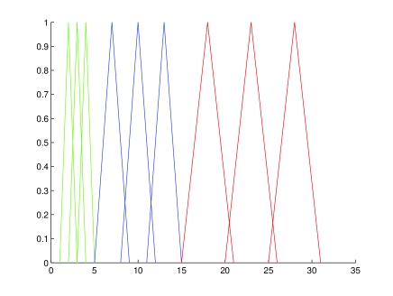
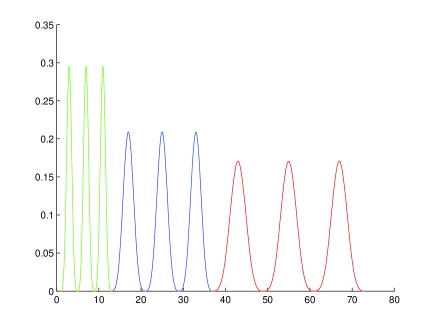
We shall focus on the particular cases corresponding to $m=2$ and $m=4$. For $m=2$ the cardinal spline space $S_{2}(\Delta)$ is the space of piece wise linear functions and can be spanned by a linear B-spline basis arising by translating the prototype function known as ‘hat’ function. The first 3 functions in the left graph of Fig. 1 are 3 consecutive linear B-spline basis functions. The 3 middle functions in the same graph are linear B-spline functions of broader support taking from a dictionary spanning the same space as the basis. The last 3 functions are taking from another dictionary for the same space. Details on how to build these dictionaries are given in [2]. The basis and dictionary functions equivalent to the ones in the left graph of Fig. 1, but for cubic spline spaces corresponding to $m=4$, are given in the right graph of the same Figure.

Figure 2: Tree splines taken from dictionaries spanning the same space. Linear splines (left) Cubic splines (right)

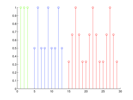
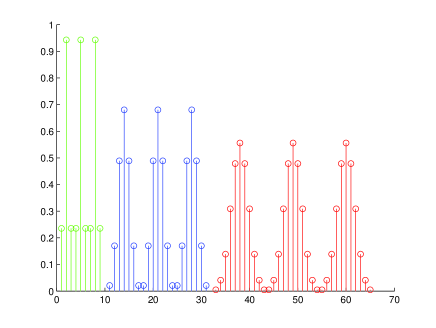
For constructing redundant dictionaries suitable for processing images by nonlinear techniques we need to make sure that the dictionaries can be processed with digital computers having the existing memory capacity. Thus, we need to a)discretise the functions to obtain adequate Euclidean vectors and b)restrict the functions to small intervals allowing for processing the images in small blocks. We carry out the discretization by taking the value of a prototype function only at the knots (cf. small circles in graphs Fig.  2) and translating that prototype one sampling point at each translation step. In regard to the boundaries one may take different routes: A possibility is to adopt periodicity (cyclic boundary conditions) and other apply the ‘cut off’ approach and keep all the vectors whose support has nonzero intersection with the interval being considered. The former would leave a basis for the corresponding Euclidean space and the later a redundant dictionary.

Remark 1.

We notice that by the proposed discretization the hat B-spline basis for the corresponding interval becomes the standard Euclidean basis for either boundary conditions. By discretizing the hats of broader support the samples preserve the hat shape.

Obviously for a finite dimension Euclidean space we can construct arbitrary dictionaries. In particular, different B-spline based dictionaries each of which comprising vectors of different support. Furthermore, we can include vectors of different support by merging dictionaries. There is, of course, a compromise between redundancy and complexity that needs to be considered. The discussion of such a tradeoff is postponed to Sec. 4, where the numerical examples are described.

From discrete unidimensional B-spline based dictionaries we obtain bidimensional ones simply by taking tensor product. Actually in Sec. 4 we consider a dictionary consisting of unidimensional cosine and B-spline based vectors, of redundancy approximately five, and build the bidimensional one by taking the tensor product of the whole dictionary with itself.

3 Implementation of the greedy algorithm OMP

The OMP technique [11] is an adaptive greedy strategy for selecting atoms which evolves as follows: Let $f\in\mathbb{R}^{N}$ be a given signal and $\{v_{i}\}_{i=1}^{L}$ a given redundant dictionary. Setting $R^{1}=f$ at iteration $k+1$ the OMP algorithm selects the atom, $v_{l_{k+1}}$ say, as the one minimizing the absolute values of the inner products $\langle v_{i},R^{k}\rangle,\,i=1,\ldots,L$, i.e.,

$$v_{l_{k+1}}=\arg\max\limits_{i\in J}|\langle v_{i},R^{k}\rangle|,\quad\text{where}\quad R^{k}=f-\sum_{i=1}^{k}c_{i}^{k}v_{\ell_{i}},$$ (2)

and $J$ is the set of indices labeling the dictionary’s atoms. The coefficients $c_{i}^{k},\,i=1,\ldots,k$ in the above decomposition are such that $||f-R^{k}||^{2}$ is minimum, which is equivalent to requesting $R^{k}=\hat{P}_{V_{k}}f$, where $\hat{P}_{V_{k}}$ is the orthogonal projection operator onto $V_{k}={\mbox{\rm{span}}}{\{v_{\ell_{i}}\}_{i=1}^{k}}$. We base our implementation for determining the coefficients $c_{i},\,i=1,\ldots,k$ on Gram Schmidt orthogonalization with re-orthogonalization, and recursive biorthogonalization. Basically, at each iteration we update the vectors

$$\tilde{v}_{i}^{k+1}=\tilde{v}_{i}^{k}-\tilde{v}_{k+1}^{k+1}\langle v_{\ell_{k+1}},\tilde{v}_{i}^{k}\rangle,$$

where $\tilde{v}_{k+1}^{k+1}=q_{k+1}/\|q_{k+1}\|^{2}$, with $q_{k+1}=v_{\ell_{k+1}}-\hat{P}_{V_{k}}q_{k+1}$ and $q_{1}=v_{\ell_{1}}$. One reorthogonalization step implies to recalculate $q_{k+1}$ as $q_{k+1}=q_{k+1}-\hat{P}_{V_{k}}q_{k+1}$. The projector $\hat{P}_{V_{k}}$ is here computed as $\hat{P}_{V_{k}}=Q_{k}Q_{k}^{\ast}$ where the $k$-columns of matrix $Q_{k}$ are the vectors $q_{i}/\|q_{i}\|,\,i=1,\ldots,k$ and $Q_{k}^{\ast}$ indicates the transpose conjugate of $Q_{k}$. However, to calculate the coefficients of the linear superposition we express the projectors as $\hat{P}_{V_{k}}={A_{k}B_{k}^{\ast}}$ where the $k$-columns of matrix $A_{k}$ are the selected vectors and the $k$-columns of matrix $B_{k}$ are the vectors $\tilde{v}_{i}^{k},\,i=1,\ldots,k$. Thus, the required coefficients arise from the inner products $c_{i}^{k}=\langle\tilde{v}_{i}^{k},f\rangle,\,i=1,\ldots,k$. Details on this type of implementation are given in [12, 4] and the code can be found at [1]. Moreover, as will be discussed in the next section, the fact that we deal with dictionaries involving DC and supported atoms reduces the general complexity of the OMP method.

4 Sparse image representation by Discrete Cosine and B-spline based dictionaries

Here we present the examples of the gain in sparsity that are achieved by using dictionaries which are the union of Discrete Cosine an B-Spline based dictionaries. In order to apply the OMP approach on an image using dictionaries of theses types is necessary to divide the image into blocks. The size of all the test images we consider is $512\times 512$ and we divide each image into blocks of $16\times 16$ pixels. For approximating each block we first construct the dictionaries ${\mathcal{D}_{1}}$ and ${\mathcal{D}_{i}},\,i=2,\ldots,4$ defined as follows

• Discrete Cosine Dictionary

  $$\mathcal{D}_{1}=\{c_{i}\cos(\frac{\pi(2j-1)(i-1)}{4L}),\,j=1,\ldots,N\}_{i=1}^{M},$$

  with $c_{i}=\frac{1}{\sqrt{L}}\,i=1,\ldots,M$ and $c_{1}=\frac{1}{\sqrt{2L}}$ a normalization factor.

• Discrete B-Spline based dictionaries

  $$\mathcal{D}_{k}=\{w_{i}B^{k}_{m}(j-i)|L;j=1,\ldots,L\}_{i=1}^{M_{k}},$$

  where the notation $B_{m}(j-i)|L$ indicates the restriction to be an array of size $L$, indices $k=2,\ldots,4$ label the dictionaries of different support and $w_{i},\,i=1,\ldots,M_{k}$, with $M_{k}$ equal to the number of atoms in dictionary $k$, are normalization constants. Considerations are limited to the cases $m=2$ (hat atoms) and $m=4$ (atoms arising by discretizing cubic splines). Because we adopt the cut off approach for the boundary, the numbers $M_{k}$ of total atoms in the $k$th-dictionary varies according to the atom’s support. For the linear spline based dictionaries the corresponding supports are: 1, 3, and 5, while for the cubic are 3, 7, and 11.

With these dictionaries we construct the tensor product dictionary $\mathcal{D}=\mathcal{D}_{i}\otimes\mathcal{D}_{j},\,i,j=i,\ldots,4$ which implies, approximately, a redundancy of five. However, the redundancy does not modify significantly the complexity order. The complexity of applying the OMP approach is dominated by the evaluation, at each iteration, of the inner products between the residual and the dictionary atoms. In the case of the proposed dictionaries the inner product with the DC dictionaries can be implemented by fast DCT and the complexity in computing the inner products with the other atoms depends on the atoms support (cf (2)). By denoting $d_{i}$ to the support of the spline based dictionary $i$, the complexity of computing the inner products at the selection step (2) is

$$O((2N)^{2}\log_{2}2N)+O(N\sum_{i=2}^{4}d_{i}M_{i}).$$

For the supported atoms we are considering the number of atoms $M_{i},\,i=2,\dots,4$ is not much larger than $N$. Moreover, for the hats dictionaries $d_{1}=1$, $d_{2}=3$ $d_{3}=5$, so that the redundancy do not affect so much the stepwise complexity dominated by the inner products of the residual with all the dictionary’s atoms. In addition which can be also accelerated by parallel calculations. Of course, the total complexity depends on the sparsity, as the complexity for selecting each atom has to be multiplied by the number of selected atoms, which is the feature of stepwise Pursuit Strategies. Nevertheless, the fact that the image is processed in small blocks leaves room for fast implementation by parallel processing.

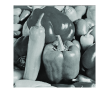
As can be observed in Table I, the performance in sparsity that is achieved with the proposed dictionaries is slightly better when using hats dictionaries, but with both dictionaries the sparsity in representing the six test images is about double than that yielded by faster nonlinear techniques such as DCT and WT.

Figure 3: The six test images from left to right, top to bottom: Boat, Bridge, Film clip, Lena, Mandril, Peppers

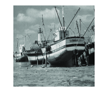
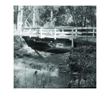
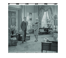
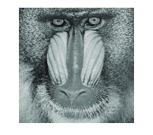
Image	DCT2 $\cup$ Linear Splines	DCT2 $\cup$ Cubic Splines	DCT	Wavelets
Boat	7.05	6.89	3.63	3.65
Bridge	4.24	3.97	2.06	2.2
Film	9.72	9.26	4.53	4.8
Lena	11.78	11.7	6.5	6.97
Mandril	3.72	3.5	1.91	1.90
Peppers	8.9	8.62	4.36	3.39

Table 1: Compression ratio (corresponding to PNSR=40 dB) achieved by each dictionary. The first column corresponds to the dictionary $\mathcal{D}_{1}$ composed of DC redundancy 2 and linear spline atoms of support 1, 3 and 5. The second column corresponds to dictionary $\mathcal{D}_{2}$ and cubic spline atoms of support 3, 7 and 11. The third column corresponds to the result obtained by nonlinear selection of DCT coefficients. The last column is the compression ratio produced by the Cohen-Daubechies-Feauveau 9/7 wavelet transform computed with the software WaveletCDF97 by thresholding coefficients so as to achieve the required PNSR or 40 dB)

5 Conclusions

Mixed DC and spline based dictionaries for sparse image representation have been introduced. It was shown that, comparing with fast nonlinear DCT and WT approaches, the proposed dictionaries yield a significant gain in sparsity. The complexity analysis and the fact that the processing is suitable for parallel computing lead to conclude that the proposed dictionaries can be of assistance to those image processing applications that benefit from the sparsity property of a representations.

References

- [1] Highly nonlinear approximations for sparse signal representation. http://www.ncrg.aston.ac.uk/Projects/HNLApprox, 2009.
- [2] M. Andrle and L. Rebollo-Neira. Cardinal B-spline dictionaries on a compact interval. Applied and Computational Harmonic Analysis, 18:336–346, 2005.
- [3] M. Andrle and L. Rebollo-Neira. Improvement of orthogonal matching pursuit strategies by backward and forward movements. In Proc. of the 31st International Conference on Acoustics, Speech, and Signal Processing, volume 3, pages III–III, 2006.
- [4] M. Andrle and L. Rebollo-Neira. A swapping-based refinement of orthogonal matching pursuit strategies. Signal Processing, 86:480–495, 2006.
- [5] S.S. Chen, D.L. Donoho, and M.A. Saunders. Atomic decomposition by basis pursuit. SIAM Journal on Scientific Computing, 20:33–61, 1998.
- [6] D. Donoho and X. Huo. Uncertainty principles and ideal atomic decomposition. EEE Transactions on Information Theory, 47:2845–2862, 2001.
- [7] R. Gribonval and M. Nielsen. Sparse representations in unions of bases IEEE Transactions on Information Theory, 49, 2003.
- [8] M. Elad M. Aharon and A.M. Bruckstein. K-svd: An algorithm for designing of overcomplete dictionaries for sparse representation. IEEE Trans on Signal Processing, 54:4311–4322, 2006.
- [9] S. Mallat and Z. Zhang. Matching pursuits with time-frequency dictionaries. IEEE Transactions on Signal Processing, 41:3397–3415, 1993.
- [10] B.A. Olshausen and B.J. Field. Emergence of simple-cell receptive field properties by learning a sparse code for natural images. Nature, 381:607–609, 1997.
- [11] Y.C. Pati, R. Rezaiifar, and P.S. Krishnaprasad. Orthogonal matching pursuit: recursive function approximation with applications to wavelet decomposition. In Proceedings of the 27th Annual Asilomar Conference in Signals, System and Computers, volume 1, pages 40–44, 1993.
- [12] L. Rebollo-Neira and D. Lowe. Optimized orthogonal matching pursuit approach. IEEE Signal Processing Letters, 9:137–140, 2002.