Neutrino Interactions Importance to Nuclear Physics

Abstract

We review the general interplay between Nuclear Physics and neutrino-nucleus cross sections at intermediate and high energies. The effects of different reaction mechanisms over the neutrino observables are illustrated with examples in calculations using several nuclear models and ingredients.

As motivation for the more specific workshop sessions, in this talk we introduce the general formalism of neutrino scattering from nuclei and define the observables of interest for nuclear physics at the energy regime of interest. Using different nuclear models we present with examples the theoretical ingredients of relevance for neutrino reactions: long Range nuclear correlations (RPA), final state interactions (FSI), finite-size effects, Coulomb corrections, and relativistic effects. Theoretical results will be shown for charge-changing quasielastic neutrino scattering. We skip here the discussion on neutral current scattering, Delta excitation and coherent pion production, which will be summarized in the M.B. Barbaro and E. Hernandez papers in these proceedings. We present results for kinematics going from low to high energy and for different kind of observables: response functions, inclusive cross sections, integrated cross sections, angular distributions, polarization observables, etc. Nuclear models for which we will show results are Local Fermi Gas (LFG), Relativistic Fermi Gas (RFG), Semi-relativistic Shell Model (SR-SM), and Super-Scaling Analysis (SuSA) model. We also skip the discussion on the Relativistic Mean Field, which will be summarized in the talk by J.M. Udias in these same proceedings. Some particular topics that we briefly discuss are theoretical uncertainties on the ratios of interest for experiments on atmospheric neutrinos, nuclear effects on lepton polarization, and reconstruction of neutrino cross section from electron scattering data.

0.1 Formalism

We consider as example the CC neutrino reaction $\nu_{l}+A\rightarrow l^{-}+B$, for initial $K^{\mu}$ and final $K^{\prime}{}^{\mu}$ lepton momenta, with energies $\epsilon$ and $\epsilon^{\prime}$, respectively. We introduce also the momentum transfer $Q^{\mu}=K^{\mu}-K^{\prime}{}^{\mu}=P^{\prime}{}^{\mu}-P^{\mu}$. It is convenient to define the following adimensional variables $\lambda=\frac{\omega}{2m_{N}}$, $\kappa=\frac{q}{2m_{N}}$, and $\tau=\kappa^{2}-\lambda^{2}$.

The inclusive cross section for the inclusive $(\nu_{l},l^{-})$ reaction where only the final lepton is detected, can be written as

$$\frac{d\sigma}{d\Omega^{\prime}d\epsilon^{\prime}}=\frac{G^{2}\cos^{2}\theta_{c}}{2\pi^{2}}k^{\prime}\epsilon^{\prime}\cos^{2}\frac{\tilde{\theta}}{2}{\cal F}_{+}^{2}\$$

Where the coupling constant $G=1.1664\times 10^{-5}\rm GeV^{-2}$, the Cabibbo angle $\theta_{c}=0.974$, and the generalized scattering angle is defined by $\tan^{2}\frac{\tilde{\theta}}{2}=\frac{|Q^{2}|}{(\epsilon+\epsilon^{\prime})^{2}-q^{2}}.$ The interesting nuclear information is contained in the structure function

$${\cal F}_{+}^{2}=\widehat{V}_{CC}R_{CC}+2\widehat{V}_{CL}R_{CL}+\widehat{V}_{LL}R_{LL}+\widehat{V}_{T}R_{T}+2\widehat{V}_{T^{\prime}}R_{T^{\prime}}.$$

The kinematic factors $\widehat{V}_{K}$, coming from the leptonic tensor, are defined by Ama05b

$$\widehat{V}_{CC}=1-\delta^{2}\tan^{2}\frac{\tilde{\theta}}{2},\kern 28.45274pt\widehat{V}_{LL}=\frac{\omega^{2}}{q^{2}}+\left(1+\frac{2\omega}{q\rho^{\prime}}+\rho\delta^{2}\right)\delta^{2}\tan^{2}\frac{\tilde{\theta}}{2},\kern 28.45274pt\widehat{V}_{CL}=\frac{\omega}{q}+\frac{\delta^{2}}{\rho^{\prime}}\tan^{2}\frac{\tilde{\theta}}{2}$$

$$\widehat{V}_{T}=\tan^{2}\frac{\tilde{\theta}}{2}+\frac{\rho}{2}-\frac{\delta^{2}}{\rho^{\prime}}\left(\frac{\omega}{q}+\frac{1}{2}\rho\rho^{\prime}\delta^{2}\right)\tan^{2}\frac{\tilde{\theta}}{2},\kern 28.45274pt\widehat{V}_{T^{\prime}}=\frac{1}{\rho^{\prime}}\left(1-\frac{\omega\rho^{\prime}}{q}\delta^{2}\right)\tan^{2}\frac{\tilde{\theta}}{2}$$

where the following adimensional variables are introduced: $\delta=\frac{m^{\prime}}{\sqrt{|Q^{2}|}},$ $\rho=\frac{|Q^{2}|}{q^{2}}$, and $\rho^{\prime}=\frac{q}{\epsilon+\epsilon^{\prime}}$.

Finally the following five nuclear weak response functions appear

$$R_{CC}=W^{00}, R_{LL}=W^{33}, R_{CL}=-\frac{1}{2}\left(W^{03}+W^{30}\right)$$

$$R_{T}=W^{11}+W^{22} R_{T^{\prime}}=-\frac{i}{2}\left(W^{12}-W^{21}\right)$$

as linear combinations of the weak CC hadronic tensor.

$$W^{\mu\nu}=\overline{\sum_{fi}}\delta(E_{f}-E_{i}-\omega)\langle f|J^{\mu}({\bf q})|i\rangle^{*}\langle f|J^{\nu}({\bf q})|i\rangle$$

where the matrix elements of the hadronic current are taken between the initial and final hadronic states in the nuclear transition $|i\rangle\rightarrow|f\rangle$. The hadronic current for a single nucleon is of the form $V-A$

$$\hat{J}_{\mu}=\overline{u}_{p}({\bf p}^{\prime})\left[F_{1}(Q^{2})\gamma_{\mu}+F_{2}(Q^{2})i\sigma_{\mu\nu}\frac{Q^{\nu}}{2m_{N}}-G_{A}(Q^{2})\gamma_{\mu}\gamma_{5}-G_{P}(Q^{2})\frac{Q_{\mu}}{2m_{N}}\gamma_{5}\right]u_{n}({\bf p})$$ (1)

0.2 The Relativistic Fermi Gas (RFG)

As example of the above general formalism in a many-nucleon system, we present here the nuclear response functions in the RFG, where the initial and final nucleons are described as (relativistic) plane waves. For the inclusive $(\nu_{l},l^{-})$ reaction we can write the five response functions as

$$R_{K}=N\Lambda_{0}U_{K}f_{RFG}(\psi)=G_{K}f_{RFG}(\psi),\quad K=CC,CL,LL,T,T^{\prime},$$ (2)

Here $N$ is the neutron number, and we have defined $\Lambda_{0}=\frac{\xi_{F}}{m_{N}\eta_{F}^{3}\kappa}$, with $\eta_{F}=k_{F}/m_{N}$ is the Fermi momentum in units of the nucleon mass, and $\xi_{F}=\sqrt{1+\eta_{F}^{2}}-1$ is the Fermi kinetic energy measured in the same units All the response functions are proportional to the RFG Scaling function $f_{RFG}(\psi)=\frac{3}{4}(1-\psi^{2})\theta(1-\psi^{2})$, that depends only on the scaling variable

$$\psi=\frac{1}{\sqrt{\xi_{F}}}\frac{\lambda-\tau}{\sqrt{(1+\lambda)\tau+\kappa\sqrt{\tau(1+\tau)}}}$$ (3)

Explicit expressions can be obtained for the single-nucleon responses $U_{K}$ Ama05b .

0.3 The Local Fermi Gas (LFG)

As an extension of the constant-density Fermi gas, the LFG is an easy model to include non-trivial nuclear effects Nie04 . It is based on the local density Approximation (LDA), with a local Fermi momentum is $k_{F}(r)=(3\pi^{2}\rho(r))^{1/3}$. The responses are averaged over the nuclear interior, weighted by the nucleon density $\rho(r)$. In this model one can easily include relevant nuclear effects such as the correct energy balance RPA nuclear correlations, Coulomb distortion, and FSI effects.

While the LFG correctly takes into account Pauli-blocking effects, it gives a wrong energy balance for the nuclear excitations. The energy balance can be corrected by the minimum nuclear excitation energy gap $Q=M(X_{f})-M(X_{i})$, instead of the usual LFG value $Q_{LFG}(r)=E_{F}^{p}(r)-E_{F}^{n}(r)$. That is equivalent to replacing $\omega\longrightarrow\omega-[Q-Q_{LFG}(r)]$.

The RPA series of Fig. 1 is solved by using a ph-ph interaction of Landau-Migdal, with parameters fitted to electromagnetic nuclear properties and transitions Spe80 . The RPA series can be generalized by including $\Delta$ excitations in the medium, and ph-$\Delta$h, $\Delta$-h$\Delta$h effective interactions. The sum of the RPA series is equivalent to a renormalization of the axial and vector parts of the weak hadronic tensor in the medium

Coulomb corrections can be included in the LFG by introducing the Coulomb self-energy of the final lepton $\Sigma_{C}=2\epsilon^{\prime}V_{C}(r)$ (where $V_{C}(r)$ is the nuclear Coulomb potential) in the charged lepton propagator, $\frac{1}{k^{2}-m_{l}^{2}-2k_{0}V_{C}(r)+i\epsilon}$. A new local energy-momentum relation for the final lepton is then obtained, that is used in the LFG calculation. This procedure is equivalent to the modified effective momentum approximation.

LFG results for ¹²C$(\nu_{\mu},\mu^{-})$ and ¹²C$(\nu_{e},e^{-})$ are presented in Fig 1, and are compared with experimental data Aue02 ; Ath97 in Table 1. The LFG with correct energy balance (Pauli+Q), over-estimates the data, while a good agreement is achieved once RPA and Coulomb corrections are included.

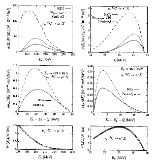
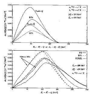
Figure 1: Left: LFG predictions for neutrino reactions from ¹²C. Left panels: $(\nu_{\mu},\mu^{-})$. Right panels: $(e,\nu_{e})$. Pauli+Q are the LFG results with correct energy balance. RPA are the results with RPA and Coulomb corrections. Top panels: total cross sections multiplied by the neutrino fluxes of the bottom. Middle panels: differential cross section for fixed neutrino energy. Right top: $\nu_{e}$ and $\overline{\nu}_{e}$ differential cross section for fixed momentum transfer; right bottom: effect of the FSI over the neutrino cross section, with and without RPA.

	Pauli+Q	RPA	LSND
$(\nu_{\mu},\mu^{-})$	20.7	11.9	$10.6\pm 0.3\pm 1.8$
$(e,\nu_{e})$	0.19	0.14	$0.15\pm 0.01\pm 0.01$

Table 1: Flux averaged neutrino cross section from ¹²C in $10^{-40}$ cm². The experimental data are from LSND Aue02 ; Ath97 .

Final State Interaction (FSI) can be taken into account in the LFG model by using a renormalized nucleon propagator in the medium $G_{FSI}(p)=\frac{1}{p^{0}-E(\vec{p})-\Sigma(p)}$, where $\Sigma(p)$ is the nucleon self-energy in the medium. A good approximations for intermediate energies is to take ${\rm Im}\Sigma_{h}\simeq 0$ for hole states. The nucleon self energy can be computed by diagrammatic techniques Fer92 . As shown in Fig. 1, the FSI importantly changes the shape of the differential cross section. The main effect is is an enhancement of the high energy tail and a reduction of the cross section at the peak region. In the same figure we also show that the RPA corrections are less important in presence of FSI.

Theoretical uncertainties in the LFG model have been computed assuming central values and errors of the model input parameters, and including 10% uncertainties in both the real part of the nucleon self-energy and densities Val06 . A Montecarlo simulation is then performed by generating sets of input parameters using Gaussian distributions. After computing the different observables, one obtains the distribution of the observable values, and the theoretical errors are identified by discarding the highest and lowest 16% of the obtained values, keeping a 68% confidence level interval. Uncertainties on the integrated cross sections are of the order of 10-15%, which turn out to be similar to those assumed for the input parameters. As shown in Fig. 3, theoretical errors cancel partially out in the ratio $\frac{\sigma(\mu)}{\sigma(e)}=\frac{\sigma(\nu_{\mu},\mu)}{\sigma(\nu_{e},e)}$ of interest for experiments on atmospheric neutrinos.

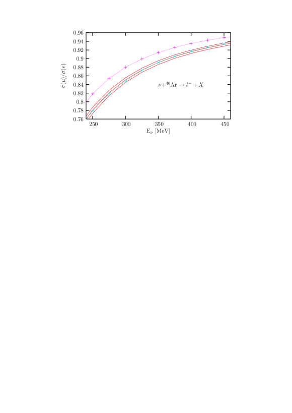
Figure 2: Ratio of inclusive cross sections $\frac{\sigma(\mu)}{\sigma(e)}$ for argon. The 68% confidence level band is displayed for the full LFG model including RPA, Coulomb and FSI. We also show results with the bare Fermi gas model without nuclear corrections.

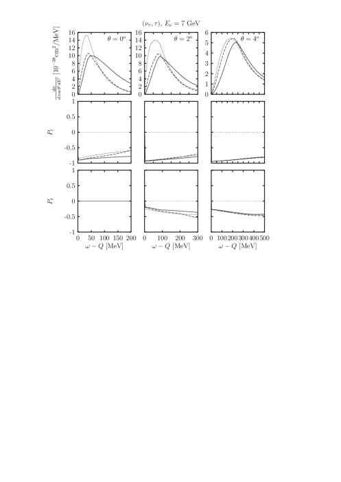
Figure 3: Polarization observables in the LFG (dotted), adding RPA correlations (dashed), and adding FSI (solid).

0.4 Polarization observables

The study of final $\tau$ polarization in $(\nu_{\tau},\tau)$ reactions Val06b is of interest for $\nu_{\mu}\longrightarrow\nu_{\tau}$ oscillation experiments. The $\tau$ decay particle distribution depend on the $\tau$ spin direction, and thus theoretical information on the $\tau$ polarization will be valuable Mig03 . Information about $\tau$ polarization is also needed in $\nu_{\mu}\longrightarrow\nu_{e}$ oscillation experiments to disentangle $(\nu_{e},e)$ events from background electron productions following the $\nu_{\mu}\longrightarrow\nu_{\tau}$ oscillation Hag03 .

The polarized differential cross section in $(\nu_{l},\vec{l})$ reactions when the final lepton polarization is measured in the direction $\vec{s}$ can be written as

$$\Sigma(\vec{s})\equiv\frac{d^{2}\sigma}{d\Omega^{\prime}dE^{\prime}_{l}}=\frac{1}{2}\Sigma_{0}\left(1+s_{\mu}P^{\mu}\right)$$

where $\Sigma_{0}$ is the unpolarized cross section. The lepton polarization vector components $P_{l}$ (longitudinal component, in the direction of the final lepton), and $P_{t}$ (transverse component in the scattering plane) can be obtained as asymmetries

$$s_{\mu}P_{\mu}=\frac{\Sigma(\vec{s})-\Sigma(\vec{-s})}{\Sigma(\vec{s})+\Sigma(\vec{-s})}.$$

Results for the polarization observables with the LFG model are shown in Fig. 4, with the differential cross section, the two $\tau$ polarization components, and the total polarization and angle. The nuclear RPA and FSI effects are of small importance at the quasielastic peak region because of partial cancellation when computing the asymmetries. Their importance increases in the tail of the cross section.

0.5 Super-Scaling Analysis (SuSA)

In the RFG, Eqs. (2,3), all the response functions can be factorized in a single-nucleon function times the superscaling function $f_{RFG}$, which only depends on the scaling variable $\psi$ and is the same for all nuclei. We then say that the RFG superscales, namely $f_{RFG}$ does not explicitly depends upon the momentum transfer $q$ (scaling of the first kind) nor the Fermi momentum $k_{F}$ (scaling of the second kind). Moreover the scaling function is the same for electron and neutrino scattering, hence the neutrino and electron cross sections are related just by a single-nucleon factor.

These ideas have been extended to extract an “experimental” scaling function from $(e,e^{\prime})$ data by computing the ratio

$$f_{exp}(\psi^{\prime})=\frac{\displaystyle\left(\frac{d\sigma}{d\Omega^{\prime}d\epsilon^{\prime}}\right)_{exp}}{\sigma_{Mott}(v_{L}G_{L}+v_{T}G_{T})}$$

where $\psi^{\prime}$ is the scaling variable shifted to account for an energy binding parameter $E_{s}$. An extensive analysis of $(e,e^{\prime})$ data has been performed in the quasielastic peak Mai02 . The parameters $k_{F}$ y $E_{s}$ are fitted to the data to minimize the differences between scaling functions for different kinematics and nuclei. When this analysis is performed on the experimentally available longitudinal, $f_{L}=\frac{R_{L}}{G_{L}}$, and transverse, $f_{T}=\frac{R_{T}}{G_{T}}$, response functions, one finds that the L response function superscales quite well, while scaling is broken in the T response above the peak, due to non-quasielastic processes (pion production, $\Delta$ excitation, MEC, etc). The experimental scaling function is shown in Fig. 6 below

Figure 4: Scaling properties of the SR shell model. Left: scaling of the first kind. Curves for $q=0.5,0.7,1,1.3,1.5$ GeV collapse into one. Right: scaling of the second kind. Curves for ¹²C, ¹⁶O and ⁴⁰Ca collapse into one

Having succeeded in representing the $(e,e^{\prime})$ quasielastic data by means of an universal superscaling function, the SuSA procedure can be reversed and give predictions for neutrino reactions Ama05 . In fact, starting with the experimental $(e,e^{\prime})$ scaling function one can use the RFG equations (2) to compute the $(\nu_{l},l^{-})$ response functions with the substitution $f_{RFG}(\psi)\longrightarrow f_{exp}(\psi)$. The assumption underlying this procedure is that the superscaling function associated to the 5 weak responses is the same and is equal to the longitudinal electromagnetic response function. Calculations aiming to to justify theoretically the validity of SuSA are presented in the next section.

0.6 The semirelativistic shell model (SRSM)

In order to study the scaling properties in realistic models one needs to go beyond the simplicity of the Fermi gas, where scaling holds by construction. In the continuum shell model (CSM), i.e., nucleons in a mean field, distortion of the ejected nucleon is present and a general proof of scaling cannot be provided. Thus, at least within the context of the CSM, we shall be able to check the consistency of the SuSA approach and quantify the degree to which scale breaking effects are expected to enter.

In the CSM the initial state $|i\rangle$ is described by a Slater determinant with all shells occupied, while in the impulse approximation the final states are particle-hole excitations coupled to total angular momentum $|f\rangle=|(ph^{-1})J\rangle$. The single hole wave function is then written as $|h\rangle=|\epsilon_{h}l_{h}j_{h}\rangle$ while the single particle wave function $|p\rangle=|\epsilon_{p}l_{p}j_{p}\rangle$. The radial functions are obtained by solving the Schrödinger equation with a Woods-Saxon potential.

At the ongoing and next generation neutrino experiments the neutrino beam energies increase to the GeV level and, typically, large energies and momenta are transferred to the nucleus. For these kinematics, relativity is important. The relevant relativistic corrections can be easily implemented in the CSM through the semi-relativistic approach (SR) Ama05b . It is based on a new expansion of the relativistic single-nucleon current $j^{\mu}(\vec{p^{\prime}},\vec{p})=\overline{u}(\vec{p^{\prime}})\Gamma^{\mu}(Q)u(\vec{p})$ in powers of the initial nucleon momentum, $\vec{\eta}=\vec{p}/m_{N}$, to first order $O(\eta)$. We do not expand in $\vec{p^{\prime}}/m_{N}$, hence $q$ and $\omega$ can be arbitrarily large. Second one must use relativistic kinematics. The energy transfer in the CSM is the difference between the (non-relativistic) single-particle energies of particle and hole $\omega=\epsilon_{p}-\epsilon_{h}$. The relativistic kinematics are taken into account by the substitution $\epsilon_{p}\rightarrow\epsilon_{p}(1+\epsilon_{p}/2m_{N})$ as the eigenvalue of the Schrödinger equation for the particle in the continuum.

A test of the SR approach was performed in Ama05b by comparing the exact RFG results with those of the SR Fermi gas model, where the above SR current and relativistic kinematics have been implemented.

An study of superscaling properties of the SRSM, for $q>0.5$ GeV/c, is performed in Fig. 4. Scaling of both first and second kind are achieved in the shell model: all the curves collapse into one with small deviations for $q=0.5$ GeV. Since both kind of scaling are found, we conclude that superscaling occurs within our model.

The SRSM with Woods-Saxon potential fails to reproduce the experimental scaling function, giving results similar to the RFG, with the exception of small tails for low and high energy transfer. The next step Ama07 is to improve the relativistic description of the ejected nucleon. The FSI is modified by using a Dirac-equation based potential plus Darwin term (DEB+D) in the final state, instead of the usual Woods-Saxon potential. The trick is to rewrite the Dirac equation as a second-order equation for the upper component $\psi_{up}(\vec{r})$. The Darwin term is then defined by: $\psi_{up}(\vec{r})=K(r,E)\phi(\vec{r})$, where the function $\phi(\vec{r})$ verifies the Schrödinger equation

$$\left[-\frac{1}{2m_{N}}\nabla^{2}+U_{DEB}(r,E)\right]\phi(\vec{r})=\frac{E^{2}-m_{N}^{2}}{2m_{N}}\phi(\vec{r}).$$

Both the DEB potential $U_{DEB}(r,E)$ and Darwin term $K(r,E)$ are energy-dependent functions. The scaling functions computed using the DEB+D potential are compared to the exact RMF results in Fig. 5. Both models give similar results, and clearly different to the SR model based on a Woods-Saxon potential.

Figure 5: Scaling functions computed in the SR shell model compared with the relativistic mean field model (RMF). Dotted: Woods-Saxon potential. Solid: DEB+D potential. Dashed: RMF.

Figure 6: Left: Scaling of 1st kind with DEB+D potential compared with experimental data. $q=0.5$, 0.7 1.0, 1.3 and 1.5 GEV/c. Right: Test of SuSA in the SR shell model for the ¹²C$(\nu_{\mu},\mu^{-})$ reaction with neutrino energy $\epsilon=1$ GeV. Dotted: Woods-Saxon potential. Solid: DEB+D potential. Dashed: SuSA reconstruction from the computed $(e,e^{\prime})$ scaling function.

Scaling of the first kind of the SRSM with the DEB+D potential is shown in Fig. 6, where we also compare with the experimental data for $f_{L}$. The scaling is surprisingly good, taking into account that the momentum transfer ranges from 0.5 to 1.5 GeV. A q-dependent energy shift $E_{s}(q)$ is needed to bring all the curves to collapse. The $q$ dependence of $E_{s}(q)$ is linear.

A test of the SuSA reconstruction of the $(\nu_{\mu},\mu^{-})$ cross section from the $(e,e^{\prime})$ one is shown in Fig. 6. There the neutrino cross section obtained by direct computation is compared with the SuSA reconstruction from the computed $(e,e^{\prime})$ longitudinal scaling function. Both results are quite similar for scattering angle above 30^o, corresponding to intermediate to large momentum transfer. For very low scattering angle there are small differences between both procedures due to the small momentum transfers involved.

0.7 Concluding remarks

Neutrino interactions importance for nuclear physics has been illustrated with examples from a selection of neutrino reactions on nuclei using different approaches. The connection of electron and neutrino cross sections has also been analyzed within the superscaling approach. Since neutrino cross sections incorporate a richer information on nuclear structure and interactions than electron cross sections, the availability of neutrino-nucleus observables of different kinds will be valuable for the development of more precise nuclear models and nuclear interaction theories.

References

- (1) J.E. Amaro, M.B. Barbaro, J.A. Caballero, T.W. Donnelly, and C. Maieron, Phys. Rev. C 71, 065501 (2005).
- (2) J. Nieves, J.E. Amaro and M. Valverde. Phys. Rev. C 70, 055503 (2004).
- (3) J. Speth, V. Klemt, J. Wambach and G.E. Brown, Nucl. Phys. A343, 382 (1980)
- (4) L.B. Auerbach et al., Phys. Rev. C 66, 015501 (2002).
- (5) C. Athanassopoulos et al., Phys. Rev. C 55, 2078 (1997).
- (6) P. Fernadez de Cordoba and E. Oset, Phys. Rev. C 46 (1992)1697.
- (7) M. Valverde, J.E. Amaro, J. Nieves, Phys. Lett. B 638 (2006)
- (8) M. Valverde, J.E. Amaro, J. Nieves, C. Maieron, Phys. Lett. B 642 (2006) 218
- (9) P. Migliozzi, Int. J. Mod. Phys. A 18 (2003) 3877.
- (10) K. Hagiwara K. Mawatari and H. Yokoya, Nucl. Phys. B 668 (2003) 364.
- (11) C. Maieron, T.W. Donnelly and I. Sick, Phys. Rev. C 65 (2002) 025502.
- (12) J.E. Amaro, M.B. Barbaro, J.A. caballero, T.W. Donnelly, A. Molinari, and I. Sick, Phys. Rev. C 71, 015501 (2005)
- (13) J.E. Amaro, M.B. Barbaro, J.A. Caballero, T.W. Donnelly, and J.M. Udias, Phys. Rev. C 75, 034613 (2007).