Optimal Timer Based Selection Schemes

Abstract

Timer-based mechanisms are often used to help a given (sink) node select the best helper node among many available nodes. Specifically, a node transmits a packet when its timer expires, and the timer value is a monotone non-increasing function of its local suitability metric. The best node is selected successfully if no other node’s timer expires within a ‘vulnerability’ window after its timer expiry, and so long as the sink can hear the available nodes. In this paper, we show that the optimal metric-to-timer mapping that (i) maximizes the probability of success or (ii) minimizes the average selection time subject to a minimum constraint on the probability of success, maps the metric into a set of discrete timer values. We specify, in closed-form, the optimal scheme as a function of the maximum selection duration, the vulnerability window, and the number of nodes. An asymptotic characterization of the optimal scheme turns out to be elegant and insightful. For any probability distribution function of the metric, the optimal scheme is scalable, distributed, and performs much better than the popular inverse metric timer mapping. It even compares favorably with splitting-based selection, when the latter’s feedback overhead is accounted for.

I Introduction

Many wireless communication schemes benefit by selecting the ‘best’ node from the many available candidate nodes and using it for data transmission. For example, cooperative communication systems exploit spatial diversity and avoid synchronization problems among relays by selecting the relay that is best suited to forward the source’s message to the destination [1, 2, 3, 4, 5, 6, 7, 8]. Cellular systems exploit spatial diversity by making the base station transmit to (or receive from) the mobile station that has the highest instantaneous channel gain to (or from) the base station. Fairness is ensured by selecting on the basis of the channel gain divided by the average throughput or average energy consumed [9, 10]. In sensor networks, node selection helps increase network lifetime [11, 7]. In vehicular ad-hoc networks (VANETs), vehicle selection improves the speed of information dissemination by ensuring that the vehicles that rebroadcast the emergency broadcast message are far away from the source of the message [12, 13]. In some of these systems, a base station or access point (which we shall generically refer to as a ‘sink’) can help the selection process by hearing transmissions from candidate nodes and sending feedback. On the other hand, in the emergency broadcast scenario in VANETs, coordination issues make explicit feedback from a sink infeasible.

The mechanism that physically selects the best node is, therefore, an important component in many wireless systems. In all the above systems, each node maintains a local suitability metric, and the system attempts to select the node with the highest metric. In [14], an inverse metric timer-based scheme was proposed, in which a node with metric $\mu$ sets its timer as $c/\mu$, where $c$ is a constant, and transmits a packet when its timer expires. This simple solution ensures that the first node that transmits is the best node. In [2], nodes with channel gains above $\mu_{u}$ transmit at time $0$, while those with channel gains below $\mu_{l}$ transmit at time $T_{\max}$. In the interval $[\mu_{l},\mu_{u})$, the mapping is linearly decreasing. In general, to ensure that the best node transmits first, the mapping is a deterministic monotone non-increasing function [14, 2].

The timer-based selection mechanism is attractive because of its simplicity and its distributed nature. It requires no feedback during the selection process. A node only needs to include its identity in the packet that it transmits upon timer expiry. A sink, if present, only needs to broadcast a single message at the end of the selection process indicating success or failure. Depending on the application, the sink may also broadcast in the message the identity of the relay has been selected. Consequently, timer-based selection has been used in several systems such as cooperative relaying to find the best relay node [14, 3], wireless network coding [15] to find the best relays that will combine the signals transmitted by multiple sources, mobile multi-hop networks [8], VANETs [12, 13] to determine which vehicle should rebroadcast an emergency message, wireless LANs [4] to enable opportunistic channel access, and sensor networks [2, 5]. It is different from the centralized polling mechanism, in which the sink node polls each node about its metric and then chooses the best one. It also differs from the time-slotted distributed splitting algorithms [16, 17] that also ensure that the first packet that the sink successfully decodes is from the best node. The difference lies in the extensive slot-by-slot three-state (idle, collision, or success) feedback of the splitting algorithm that controls which nodes transmit in the next slot.

The timer scheme works by ensuring that the best node transmits first. However, for successful selection in practical systems, it is necessary that no other timer expires within a time window of the expiry of the best node’s timer. This time window, the vulnerability window [18], will be explained in detail in the next section. Selection failure occurs when two or more packets collide at the receiver and become indecipherable, or unequal node-to-sink propagation delays cause a packet from the best node to not arrive first at the receiver. One can decrease failure rate by increasing the size of the vulnerability window or the maximum selection duration, $T_{\max}$. However, the latter is not desirable because it reduces the time available to the selected node to transmit data. If the metrics depend on instantaneous channel fading gains, such an increase also reduces the ability of the system to handle larger Doppler spreads.

In this paper, we consider the general timer scheme in which the metric-to-timer function is monotone non-increasing. In contrast to the ad hoc mappings used in the literature, we determine the optimal mapping that maximizes the probability of success or minimizes the expected time required for selection subject to a minimum constraint on the probability of success. The former is relevant in systems that reserve a fixed amount of time for selection, e.g., [19], while the latter is relevant in systems that instead use the best node as soon as it is selected.

The specific contributions of the paper are the following. We provide a full recursive characterization of the optimal metric-to-timer mapping function, and show that it is amenable to practical implementation. We show that optimal timer schemes for the two previously stated problems set the timer expiry at only a finite number of points in time. That is, the optimal timer values are discrete. The number of points depends on the maximum allowed time for selection $T_{\max}$ and vulnerability window. In the asymptotic regime, in which the number of nodes, $k$, is large, we show that the description of the optimal scheme and its analysis simplifies remarkably, and takes an elegant and simple recursive form. The asymptotic regime turns out to be a good approximation even for $k$ as small as 5. Our results hold for all real-valued metrics with arbitrary probability distribution functions.

Compared to the inverse metric mapping, we show that the probability that the system fails to select the best node can often be substantially decreased by at least a factor of 2 for the same maximum selection duration. And, for a given probability of success, the average number of slots of the optimal scheme is less by a factor of two or more than that of the inverse timer scheme. We also show that the optimal timer scheme is scalable in that its performance does not catastrophically degrade as the number of nodes increases.

The paper is organized as follows. The system model and the general timer-based selection scheme are described in Sec. II. The optimal schemes are derived and analyzed in Sec. III and IV. Section V presents numerical simulations and compares with previously proposed schemes, and is followed by our conclusions in Sec. VI. Mathematical proofs are relegated to the Appendix.

II Timer-Based Selection: System Model and Basics

We consider a system with $k$ nodes and a sink as shown in Figure 1. The sink represents any node that is interested in the message transmitted by the $k$ nodes; it need not conduct any coordinating role. Each node $i$ possesses a suitability metric $\mu_{i}$ that is known only to that specific node. The metrics are assumed to be independent and identically distributed across nodes. The probability distribution is assumed to be known by all nodes. The aim of the selection scheme is to make the sink determine which node has the highest $\mu_{i}$, henceforth called the ‘best’ node.

Each node $i$, based on its local metric $\mu_{i}$, sets a timer $T_{i}=f(\mu_{i})$, where $f(.)$ is called the metric-to-timer function. When the timer expires (at time $T_{i}$), the node immediately transmits a packet to the sink. The packet contains the identity of the node along with other system-specific information. As mentioned, the timer-based selection scheme always ensures that the timer of a node with a larger metric expires no later than that of a node with a smaller metric. Consequently, $f(\mu)$, in general, is a monotone non-increasing function. The selection process has a maximum selection duration $T_{\max}$, after which nodes do not start a transmission.

For the sink to successfully decode the packet sent by the best node, the start time of any other packet must not be earlier than the start time of the packet of the best node plus a vulnerability window $\Delta$. Thus, the sink can decode the packet from the best node, if the timers of the best and second best node, denoted by $T_{(1)}$ and $T_{(2)}$ respectively, expire such that $T_{(2)}-T_{(1)}\geq\Delta$. The expiry of timers of other nodes, which occurs after $T_{(2)}$, does not matter since the sink is only interested in the best node.

The value of $\Delta$ depends on system capabilities. For example, $\Delta$ typically includes the maximum propagation and detection delays between all nodes. $\Delta$ may also include the maximum transmission time of packets in case carrier sensing is not used, in which case the nodes do not need to overhear other transmissions. Carrier sensing, which is commonly used today, is beneficial as it reduces $\Delta$ since a node, when its timer expires, will overhear transmissions and does not transmit if it senses another transmission. Note, however, that the timer scheme works with carrier sensing and without. For a system with half-duplex nodes, $\Delta$ may also include the receive-to-transmit switching time.

Henceforth, we will abuse the above general definition of $\Delta$ and instead say that a collision occurs when the timers of the best and the second best nodes expire within a duration $\Delta$. Thus, the best node is selected successfully if: (i) the timer value of the best node, $T_{(1)}$, is smaller than or equal to $T_{\max}$, and (ii) the transmission from the best node does not suffer from a collision. Otherwise, the best node selection process fails. The selection process stops at $T_{(1)}$ or $T_{\max}$, whichever is earlier.

In this paper, inability to select the best node is treated as a failure or an outage. In fact, if a sink is available, it may respond to a selection failure in multiple ways. For example, it may resolve the nodes whose packets collided during the selection process, using extra feedback. If a sink is not available, then repeated transmission schemes can be used to improve the overall reliability of broadcast messages. The details of how the system deals with a selection failure are beyond the scope of this paper.

To study the performance of selection schemes, we measure the probability of successful selection and the expected stop time of the selection scheme. These are clearly relevant to all systems that use selection. They motivate the following two different schemes to optimize the metric-to-timer mapping:

1. Scheme 1: Maximize the probability of success given a maximum selection duration of $T_{\max}$ and the number of nodes $k$.

2. Scheme 2: Minimize the expected selection time given a maximum selection duration of $T_{\max}$ such that the probability of success is at least $\eta$ when $k$ nodes are present.

A minimum requirement on the success probability is needed in the second scheme because otherwise a trivial scheme that makes each of its nodes set its timer to 0 would be optimal. This is undesirable because the probability of success of such a scheme is zero when $k\geq 2$.

We assume that all nodes know $k$, as is also assumed in the splitting approach in [16, 17]. This can be achieved, for example, by making the sink broadcast $k$ occasionally. The burden of this feedback is not significant since $k$ typically varies on a much slower time scale than, for example, the instantaneous channel fades. Even when the sink is not available, nodes can estimate $k$ by overhearing packet transmissions in the network.

To keep notation simple, we first consider the case where the metrics are uniformly distributed over the interval $[0,1)$. Thereafter, the results are generalized to all real-valued metrics with arbitrary probability distribution functions.

Notation: Floor and ceil operations are denoted by $\left\lfloor{.}\right\rfloor$ and $\left\lceil{.}\right\rceil$, respectively. ${\bf E}\left[{X}\right]$ denotes the expected value of a random variable (RV) $X$. Using order statistics notation [20, Chp. 1], the node with the $i$th largest metric is denoted by $(i)$. Consequently, $\mu_{(1)}\geq\mu_{(2)}\geq\cdots\geq\mu_{(k)}$ and $T_{(1)}\leq\cdots\leq T_{(k)}$. For notational convenience, the summation $\sum_{l=l_{1}}^{l_{2}}$ equals $0$ whenever $l_{1}>l_{2}$. We use the superscript ^∗ to denote an optimal value; for example, optimal value of $x$ is $x^{*}$. $\text{Pr}\left({A}\right)$ denotes the probability of an event $A$, and $\text{Pr}\left({A|B}\right)$ denotes the conditional probability of $A$ given $B$.

III Scheme 1: Maximizing The Probability of Success Given $T_{\max}$

The goal here is to find an optimal mapping $f^{*}(\mu)$ in the space of all monotone non-increasing functions $f:[0,1)\rightarrow\mathbb{R}^{+}$, that maximizes the probability of success. The following lemma shows that an optimal $f^{*}(\mu)$ maps the metrics into discrete timer values. Let $N=\left\lfloor{\frac{T_{\max}}{\Delta}}\right\rfloor$.

Lemma 1

An optimal metric-to-timer mapping $f^{*}(\mu)$ that maximizes the probability of success within a maximum time $T_{\max}$ maps $\mu$ into $(N+1)$ discrete timer values $\{0,\Delta,2\Delta,\ldots,N\Delta\}$.

Proof:

The proof is given in Appendix -A. ∎

The discreteness result is intuitively in sync with the fact that time slotted multiple access protocols are better than unslotted ones in terms of throughput. However, there is a subtle but fundamental distinction between our selection problem and the multiple access problem. While slotting is better in multiple access protocols because it reduces the vulnerability window, in our problem the vulnerability window remains unchanged. Note that the above discrete mapping, while optimal, need not be unique. For example, when $N\Delta<T_{\max}$, the highest timer value can be increased beyond $N\Delta$ without affecting the probability of success. Also, any increase in the discrete timer values that ensures that there are $(N+1)$ of them below $T_{\max}$ and are spaced at least $\Delta$ apart, achieves the same probability of success. Note also that the timer-based scheme is different from the oft-employed RTS/CTS handshaking scheme, which addresses the hidden terminal problem that may arise after the sink receives the RTS packet successfully. In fact, the timer scheme may even be used in the RTS backoff procedure to increase the success rate of RTS packet reception.

Implications of Lemma 1: We have reduced an infinite-dimensional problem of finding $f(\mu)$ over the space of all positive-valued monotone non-increasing functions to one over $N+1$ real values that lie between 0 and $T_{\max}$, as illustrated in Figure 2. To completely characterize the optimal timer scheme, all we need to specify is the contiguous metric intervals in $[0,1)$ that get assigned to the timer values $0,\Delta,\ldots,N\Delta$. As shown in Figure 2, all nodes with metrics in the interval $[1-\alpha_{N}[0],1)$, of length $\alpha_{N}[0]$, set their timers to 0. Nodes with metrics in the next interval $[1-\alpha_{N}[1]-\alpha_{N}[0],1-\alpha_{N}[0])$, of length $\alpha_{N}[1]$, set their timers to $\Delta$, and so on. In general, nodes with metrics in the interval $\left[1-\sum_{j=0}^{i}\alpha_{N}[j],1-\sum_{j=0}^{i-1}\alpha_{N}[j]\right)$, of length $\alpha_{N}[i]$, set their timer to $i\Delta$. Any node with metric less than $\left(1-\sum_{j=0}^{N}\alpha_{N}[j]\right)$ does not transmit at all. Therefore, the probability of success is entirely a function of $N$, $\alpha_{N}[0],\ldots,\alpha_{N}[N]$, and the number of nodes $k$. To keep the notation simple, we do not explicitly show its dependency on $k$. We now determine the optimal $\alpha_{N}^{*}[j]$ and fully characterize the optimal scheme.

Theorem 1

The probability of success in selecting the best node among $k$ nodes, subject to a maximum selection duration of $T_{\max}$, is maximized when the timer of a node with metric $\mu$ is

$$f^{*}(\mu)=\left\{\begin{array}[]{ll}i\Delta,&1-\sum_{j=0}^{i}\alpha_{N}^{*}[j]\leq\mu<1-\sum_{j=0}^{i-1}\alpha_{N}^{*}[j],\ \text{for}\ 0\leq i\leq N\\ T_{\max}+\epsilon,&\text{otherwise}\end{array}\right.,$$ (1)

where $N=\left\lfloor{\frac{T_{\max}}{\Delta}}\right\rfloor$ and $\epsilon$ is any arbitrary strictly positive real number. The $N+1$ interval lengths $\alpha_{N}^{*}[0],\ldots,\alpha_{N}^{*}[N]$ are recursively given by

$$\alpha_{N}^{*}[j]=\left\{\begin{array}[]{ll}\frac{1-P_{N-1}^{*}}{k-P_{N-1}^{*}},&j=0\\ \left(1-\alpha_{N}^{*}[0]\right)\alpha_{N-1}^{*}[j-1],&1\leq j\leq N\end{array}\right.,$$ (2)

where $\alpha_{0}^{*}[0]=1/k$. $P_{N}^{*}$ is the maximum probability of success that equals

$$P_{N}^{*}=k\sum_{l=0}^{N}\alpha_{N}^{*}[l]\left(1-\sum_{j=0}^{l}\alpha_{N}^{*}[j]\right)^{k-1}.$$ (3)

Proof:

The proof is given in Appendix -B. ∎

The discrete nature of the optimal scheme also makes it amenable to practical implementation. Each node only needs to store an unwrapped version of the above recursion in the form of a look up table that has $N+1$ entries $\left\{{\alpha_{N}^{*}[0],\ldots,\alpha_{N}^{*}[N]}\right\}$. The entries are a function of $k$. A node only needs to determine the interval its metric lies in and chooses the timer accordingly.

III-A Asymptotic Analysis of Optimal Scheme as $k\to\infty$ with Finite $N$

We now provide asymptotic expressions for the optimal timer scheme as the number of nodes $k\to\infty$. The maximum selection duration, $T_{\max}$, or equivalently $N$, is kept fixed. As we shall see, the recursions simplify to a simple and elegant form because a scaled version of the metric follows a Poisson process [21]. The asymptotic expressions are also relevant practically because, as we shall see, they approximate well the optimal solution of Theorem 1 for $k$ as small as 5.

From (2), it can be seen that $\alpha_{N}^{*}[j]$ tends to zero as $k\to\infty$. Therefore, for node $i$, consider a scaled metric $y_{i}=k(1-\mu_{i})$, and normalize the interval lengths to

$$\beta_{N}^{*}[j]=k\alpha_{N}^{*}[j].$$ (4)

Thus, selecting a node with highest $\mu_{i}$ is equivalent to selecting the node with the lowest $y_{i}$. Let $y_{(1)}\leq y_{(2)}\leq\cdots\leq y_{(k)}$. Define the point process $M(z)\triangleq\sup{\left\{k\geq 1:y_{(k)}\leq z\right\}}$. $M(z)$ is simply the number of nodes whose $y_{i}=k(1-\mu_{i})$ is less than $z$.

Lemma 2

The process $M(z)$ forms a Poisson process as $k\to\infty$.

Proof:

The $\{y_{i}\}_{i=1}^{k}$ are uniformly and identically distributed in $(0,k]$. Thus, $\text{Pr}\left({M(z)=l}\right)=\binom{k}{l}\left(\frac{z}{k}\right)^{l}\left(1-\frac{z}{k}\right)^{(k-l)}$, for $0\leq l\leq l$, and tends to $e^{-z}\frac{z^{l}}{l!}$ as $k\to\infty$. Thus, it follows from [21, Chp. 2] that $M(z)$ forms a Poisson process with rate 1 as $k\to\infty$. ∎

This result enables the use of the independent increments property of Poisson processes [21, Chp. 2]. Simply stated, the property says that the number of points that occur in disjoint intervals are independent of each other. We use it below to determine the optimal $\beta_{N}^{*}[j]$.

Theorem 2

The optimal $\beta_{N}^{*}[j]$ that maximize the probability of success are given by

$$\beta_{N}^{*}[j]=\left\{\begin{array}[]{ll}1,&j=N\\ 1-e^{-\beta_{N}^{*}[j+1]},&0\leq j\leq N-1\end{array}\right..$$ (5)

Also, the probability of success of the optimal scheme is $P_{N}^{*}=e^{-\beta_{N}^{*}[0]}$.

Proof:

The proof is given in Appendix -C. ∎

Theorem 2 leads to the following key insights about the optimal timer scheme.

Corollary 1 (Scalability)

As $k\to\infty$, the probability of success of the optimal scheme for any $T_{\max}$ is greater than or equal to $1/e$, with equality occurring only for $N=0$.

Proof:

This follows because $\beta_{0}^{*}[0]=1$, and $\beta_{N}^{*}[0]\leq 1$ from the recursion in (5). ∎

Corollary 2 (Monotonicity)

$\beta_{N}^{*}[0]<\beta_{N}^{*}[1]<\cdots<\beta_{N}^{*}[N]$.

Proof:

The result follows from (5) and the inequality $1-e^{-x}<x$, for $x>0$. ∎

This result reflects a behavior typical of finite horizon dynamic programming problems. In our problem, selection at a discrete time value does not happen when either a collision occurs or the best node does not transmit. As the time available decreases, the risk of selection failure due to the best node not transmitting increases. To counteract this, the monotonicity property makes the optimal scheme take on a higher risk of collision.

Corollary 3 (Independence)

$\beta_{N}^{*}[N-r]$ depends only on $r$, and is independent of $N$.

Proof:

Since $\beta_{N}^{*}[N]=\beta_{N-1}^{*}[N-1]=1$, it follows from (5) that $\beta_{N}^{*}[j]=\beta_{N-1}^{*}[j-1]$, for $j\geq 1$. This also follows from the independent increments property: given that no node exists with $y_{i}\in(0,\beta_{N}^{*}[0]]$, $M(z+\beta_{N}^{*}[0])$ is a rate 1 Poisson process, and time $(N-1)\Delta$ is left to select the best node. By arguing successively, we get $\beta_{N}^{*}[j]=\beta_{N-l}^{*}[j-l]$ for $j\geq l$. ∎

IV Scheme 2: Minimizing the Expected Selection Time

Our aim now is to minimize the expected selection time, $\Gamma_{N}$, subject to the constraint that the probability of success, $P_{N}$, exceeds $\eta$. Formally, the constrained optimization problem is:

$$\min_{f(\mu):[0,1)\rightarrow\mathbb{R}^{+}}\Gamma_{N}\quad\text{subject to}\ P_{N}\geq\eta.$$ (6)

Feasibility of Solution: For a given $T_{\max}$, a solution to the problem above exists if and only if $\eta$ is less than or equal to the optimum probability of success for Scheme 1. This is because Scheme 1, by definition, achieves the highest probability of success given $T_{\max}$. Henceforth, we shall assume that the solution is feasible. The following Lemma shows that the optimal mapping $f^{*}(\mu)$ for this problem also is discrete.

Lemma 3

The optimal metric-to-timer mapping $f^{*}(\mu)$ that minimizes the expected selection time subject to a minimum probability of success constraint, $\eta$, maps $\mu$ into $(N+1)$ discrete timer values $\{0,\Delta,2\Delta,\ldots,N\Delta\}$, where $N=\left\lfloor{\frac{T_{\max}}{\Delta}}\right\rfloor$.

Proof:

The proof is given in Appendix -D. ∎

Hence, to determine the optimal mapping, it is sufficient to look at mappings defined by the $N+1$ variables $\alpha_{N}[0],\ldots,\alpha_{N}[N]$, where a node with metric in the interval $[1-\alpha_{N}[0],0)$ sets its timer to $0$, and a node with metric in the interval $[1-\alpha_{N}[1]-\alpha_{N}[0],1-\alpha_{N}[0])$ set its timer to $\Delta$, and so on, as illustrated in Figure 2. In general, a node with metric in the interval $[1-\sum_{j=0}^{i}\alpha_{N}[j],1-\sum_{j=0}^{i-1}\alpha_{N}[j])$, of length $\alpha_{N}[i]$, set its timer to $i\Delta$. A node whose metric is less than $1-\sum_{j=0}^{N}\alpha_{N}[j]$ does not transmit at all.

Consider the minimization of an auxiliary function $L_{N}^{\lambda}\triangleq\Gamma_{N}-\lambda P_{N}$, for a given $\lambda\geq 0$. We now show that the solution that minimizes $L_{N}^{\lambda}$ is the solution of the optimization problem in (6), and that the inequality becomes an equality. Let $f^{\lambda*}(\mu)$ be the mapping with the lowest value of the auxiliary function for a given $\lambda$. Let its probability of success and expected selection time be $P_{N}^{\lambda*}$ and $\Gamma_{N}^{\lambda*}$, respectively. Consider any other feasible scheme $f^{\prime}(\mu)$ with corresponding probability of success $P_{N}^{\prime}$ and expected selection time $\Gamma_{N}^{\prime}$. Therefore, $\Gamma_{N}^{\prime}-\lambda P_{N}^{\prime}\geq\Gamma_{N}^{\lambda*}-\lambda P_{N}^{\lambda*}$. If $P_{N}^{\prime}\geq P_{N}^{\lambda*}$, then $\Gamma_{N}^{\lambda*}\leq\Gamma_{N}^{\prime}-\lambda\left(P_{N}^{\prime}-P_{N}^{\lambda*}\right)\leq\Gamma_{N}^{\prime}$ since $\lambda\geq 0$. Therefore, the expected selection time of $f^{\lambda*}(\mu)$ is the lowest among all timer mappings for which $P_{N}^{\prime}\geq P_{N}^{\lambda*}$. Consequently, if we choose $\lambda$ such that $P_{N}^{\lambda*}=\eta$, then the resulting mapping $f^{\lambda*}(\mu)$ is the solution of (6).

The following theorem specifies the optimal timer scheme as a function of $\lambda$.

Theorem 3

Given $\lambda\geq 0$, the auxiliary function $L_{N}^{\lambda}$ is minimized when a node with metric $\mu$ sets its timer as $f^{*}(\mu)$, where

$$f^{*}(\mu)=\left\{\begin{array}[]{ll}i\Delta,&1-\sum_{j=0}^{i}\alpha_{N}^{*}[j]\leq\mu<1-\sum_{j=0}^{i-1}\alpha_{N}^{*}[j],\ \text{for}\ 0\leq i\leq N\\ T_{\max}+\epsilon,&\text{otherwise}\end{array}\right.,$$ (7)

where $N=\left\lfloor{\frac{T_{\max}}{\Delta}}\right\rfloor$, $\epsilon$ is an arbitrary positive real number. $\alpha_{N}^{*}[0],\ldots,\alpha_{N}^{*}[N]$ are recursively given by

$$\alpha_{N}^{*}[j]=\left\{\begin{array}[]{ll}\frac{1+\frac{\lambda}{\Delta}-\frac{\lambda}{\Delta}L_{N-1}^{*{\lambda}}}{1+\frac{\lambda}{\Delta}k-\frac{\lambda}{\Delta}L_{N-1}^{*{\lambda}}},&j=0\\ \left(1-\alpha_{N}^{*}[0]\right)\alpha_{N-1}^{*}[j-1],&1\leq j\leq N\end{array}\right.,$$ (8)

and $\alpha_{0}^{*}[0]=1/k$. $L_{N}^{*{\lambda}}$ is the minimum value of the auxiliary function that equals

$$L_{N}^{*{\lambda}}=\Delta\sum_{l=0}^{N-1}\left(1-\sum_{j=0}^{l}\alpha_{N}^{*}[j]\right)^{k}-\lambda\sum_{l=0}^{N}\alpha_{N}^{*}[l]\left(1-\sum_{j=0}^{l}\alpha_{N}^{*}[j]\right)^{k-1}.$$ (9)

Proof:

The proof is given in Appendix -E. ∎

Note that as $\lambda/\Delta\to\infty$, $\alpha_{N}^{*}[j]$ tends to the corresponding optimal value for Scheme 1. This is intuitive because, for large $\lambda$, minimizing $L_{N}^{\lambda}$ is equivalent to maximizing $P_{N}$. Notice also that $\alpha_{N}^{*}[j]$ and $P_{N}^{*}$ depend on $\lambda$ only through the term $\lambda/\Delta$. Thus, as expected, the optimal solution, $\alpha_{N}^{*}[j]$, for the constrained problem in (6) does not depend on $\Delta$ for a given $N$; scaling $\Delta$ will accordingly scale the value of $\lambda$ to ensure $P_{N}^{*}=\eta$.

IV-A Asymptotic Behavior of Optimal Scheme as $k\to\infty$ Given $N$

We now develop an asymptotic analysis of the optimal timer scheme when $k\to\infty$. Define the normalized interval lengths: $\beta_{N}^{*}[j]=k\alpha_{N}^{*}[j]$, for $j=0,\ldots,N$. Then, the optimal $\beta_{N}^{*}[j]$ are as follows.

Theorem 4

Given $\lambda\geq 0$, the optimal values $\beta_{N}^{*}[j]$ that minimize the auxiliary function are given by the recursion

$$\beta_{N}^{*}[j]=\left\{\begin{array}[]{ll}1,&j=N\\ 1-e^{-\beta_{N}[j+1]}+\Delta/\lambda,&0\leq j\leq N-1\end{array}\right..$$ (10)

The optimum probability of success is $P_{N}^{*}=\sum_{l=0}^{N}\beta_{N}^{*}[l]e^{-\sum_{j=0}^{l}\beta_{N}^{*}[j]}$ and the expected selection time is $\Gamma^{*}_{N}=\Delta\sum_{l=0}^{N-1}e^{-\sum_{j=0}^{l}\beta_{N}^{*}[j]}$.

Proof:

The proof is given in Appendix -F. It also uses Lemma 2, which showed that the point process $M(z)=\sup{\left\{k\geq 1:y_{(k)}\leq z\right\}}$ is a Poisson process with rate 1 as $k\to\infty$. Recall that $y_{i}=k(1-\mu_{i})$ and $y_{(a)}\leq y_{(b)}$, for $a\leq b$. ∎

For both the schemes, we have $\beta_{N}^{*}[N]=1$. However, $\beta_{N}^{*}[j]$, for $0\leq j<N$, for Scheme 2 is always greater than or equal to that for Scheme 1. This is because of the additional $\Delta/\lambda$ term in (10), which increases $\beta_{N}^{*}[j]$. By decreasing $\lambda$, the expected selection time decreases and so does the probability of success. For a given $\lambda$, it can be verified that $\beta_{N}^{*}[j]$ satisfy the Independence property described in Sec. III for Scheme 1.

IV-B Generalization to Real-Valued Metrics with Arbitrary Probability Distributions

We now generalize the optimal solutions of Schemes 1 and 2 to the general case where the metric is not uniformly distributed. Let the cumulative distribution function (CDF) of a metric be denoted by $F_{c}(x)=\text{Pr}\left({\mu\leq x}\right)$, where $-\infty<x<\infty$.

The optimum mapping when the CDF of the metric is $F_{c}(.)$ is $f^{*}\left(F_{c}(\mu)\right)$, where $f^{*}(.)$ is given by Theorem 2 for Scheme 1 and by Theorem 3 for Scheme 2. This follows because $F_{c}(.)$ is a monotonically non-decreasing function, and the random variable $Y=F_{c}(\mu)$ is uniformly distributed between 0 and 1. The problem has, therefore, been reduced to the one considered earlier. This also shows that the performance for the optimal mapping for the two schemes does not depend on $F_{c}(.)$. Note here that we assume that the nodes know $F_{c}(.)$. This is also assumed in the splitting approaches [16, 17]. Practically, this is justified because $F_{c}(.)$, being a statistical property, can be computed over time.

V Results and Performance Evaluation

We now study the structure and performance of the optimum timer schemes. We also compare them with the popular inverse metric timer mapping that uses $f(\mu)=c/\mu$ [14, 3, 5, 15]. In order to ensure a fair comparison with Schemes 1 and 2, for each $T_{\max}$ and $k$, $c$ is numerically optimized to maximize the probability of success for Scheme 1 or minimize the expected selection time for Scheme 2. Unlike the optimal timer scheme, the performance of the inverse metric mapping clearly depends on the probability distribution of the metric. For this, we shall consider a unit mean Rayleigh distribution (with CDF $F_{c}(\mu)=1-e^{-\mu^{2}/2}$), which characterizes the receive power distribution in wireless channel, and a unit mean exponential distribution (with CDF $F_{c}(\mu)=1-e^{-\mu}$), which is simply the square of a Rayleigh RV.

Figure 3 plots the maximum probability of success of Scheme 1 ($P_{N}^{*}$) as a function of $N$. Also plotted are results from Monte Carlo simulations, which match well with the analytical results. It can be seen that the asymptotic curve is close to the actual curve for $k\geq 5$. The asymptotic curve shows a rather remarkable result: regardless of $k$ and without the use of any feedback, the best node gets selected with a probability of over 75% when $N$ is just 5. When $N$ increases to 17, the success probability exceeds 90%!

We also see that the optimal scheme significantly outperforms the inverse metric mapping, despite the latter’s parameters being optimized. For example, for $N=10$ and $N=30$, the probability that the system fails to select the best node for the inverse timer scheme is respectively 2.3 and 2.5 times greater than that of the optimum scheme for the exponential CDF. The factors increase to 2.9 and 3.2 for the Rayleigh CDF. Thus, even though the exponential RV is the square of the Rayleigh RV and the squaring operation preserves the metric order, the performance of the inverse timer scheme changes.

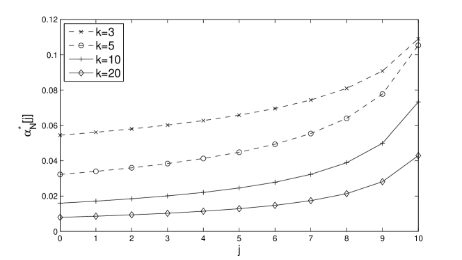
Figure 4: Scheme 1: Optimum $\alpha_{N}^{*}[j]$ as a function of $j$ and the number of nodes, $k$, for $N=10$.

The structure of the optimal Scheme 1 is studied in Figure 4, which plots $\alpha_{N}^{*}[j]$ for $N=10$ when the metric is uniformly distributed between 0 and 1. (The parameters for arbitrary distributions can be obtained using Sec. IV-B.) We see that $\alpha_{N}^{*}[j]$ increases with $j$, which is in line with the asymptotic monotonicity property of Corollary 2.

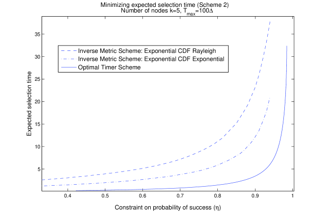
Figure 5: Scheme 2: Optimum expected selection time as a function of constraint on probability of success $(P_{N}\leq\eta)$ for $T_{\max}=100\Delta$ and $k=5$. Also, plotted is the selection time of the inverse metric mapping.

Figure 5 considers Scheme 2 and plots the optimal expected selection time as a function of the constraint on the probability of success $\eta$ for $N=100$. We again see a good match between the analytical results and the results from Monte Carlo simulations. As in Scheme 1, the optimal scheme significantly outperforms the optimized inverse metric mapping. For example, for $\eta=0.7$ and $k=5$, the optimal scheme is 5.1 and 9.6 times faster than the optimized inverse metric mapping for the exponential and Rayleigh CDFs, respectively. Again, the inverse metric mapping is sensitive to the metric’s probability distribution.

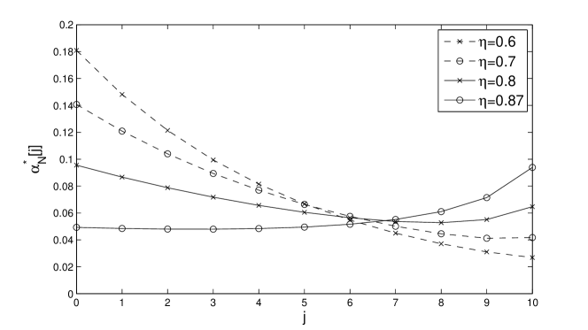
Figure 6: Scheme 2: Optimum $\alpha_{N}[j]$ as a function of $j$ and $\eta$ for $N=10$ and $k=5$.

We now study the structure of the optimal Scheme 2. Figure 6 shows the effect of the minimum success probability, $\eta$, on $\alpha_{N}^{*}[j]$ when $N=10$ and $k=5$. When $\eta$ is low, the optimal timer scheme becomes faster by tolerating a higher degree of selection failure. It maps relatively large intervals into small timer values, and is very aggressive in the beginning. Also, only a small fraction of nodes do not transmit before $T_{\max}$. For example, for $\eta=0.6$ and $N=10$, only 10.7% of nodes have timer values greater than $T_{\max}$. This result is relevant in a high mobility environment where selection needs to be fast as the metric values become outdated quickly. As $\eta$ increases, the scheme becomes conservative in order to improve its probability of success. For example, when $\eta=0.87$ and $N=10$, 37.5% of nodes, on average, do not transmit at all. As $\eta$ approaches the maximum success probability of Scheme 1, Scheme 2’s parameters converge to those of Scheme 1.

V-A Comparison with the Splitting-Based Selection Algorithm with Feedback

It is instructive to compare the optimal timer scheme with the time-slotted splitting algorithm of [16, 22] given that they both achieve the same goal but in a vastly different manner. The splitting algorithm is fast; it selects the best node within 2.467 time-slots, on average, even when $k$ is large. In it, the sink broadcasts feedback to the nodes at the end of every slot to specify whether the outcome of the transmission in the slot was an idle, a success, or a collision.

We consider, as an example, selection in IEEE 802.11 wireless local area networks [23] that use half-duplex nodes with carrier sensing capability. For the splitting algorithm, the duration of a slot, in 802.11 terminology, is $2(\text{aSIFSTime}+\text{aPreambleLength}+\text{aPLCPHeaderLength})$, where the last two terms account for a packet’s preamble and header. This is because each slot contains two transmissions, the first by one or more nodes and the second by the sink to send the 2-bit feedback (plus preambles and headers), and every transmission is followed by a small interframe space (SIFS). On the other hand, the timer algorithm requires no feedback transmission. Therefore, $\Delta=\text{aSlotTime}$, and the optimal timer scheme’s average selection time is $\Gamma^{*}_{N}$. From [23, Table 17-15], for an Orthogonal Frequency Division Multiplexing (OFDM) system with a bandwidth of 10 MHz, $\text{aSlotTime}=13~{}\mu$s, $\text{aSIFSTime}=\text{aPreambleLength}=32~{}\mu$s, and $\text{aPLCPHeaderLength}=8~{}\mu$s. Hence, the splitting algorithm’s slot duration is $144~{}\mu$s, which is 11 times the vulnerability window, $\Delta=13~{}\mu$s, of the timer scheme.

Table I shows the average selection time as a function of the probability of success constraint for the timer scheme, and compares it with splitting scheme for large $k$. Note that the splitting scheme’s probability of success is entirely determined by $T_{\max}$ and is not tunable. When $T_{\max}$ is small, the timer scheme is faster and can also achieve a higher probability of success if required. For larger $T_{\max}$, the probability of success of the splitting algorithm increases considerably; but, the timer scheme is still faster than the splitting scheme unless the probability of success required is high.

VI Conclusions

We considered timer-based selection schemes that work by ensuring that the best node’s timer expires first. Each node maps its priority metric to a timer value, and begins its transmission after the timer expires. We developed optimal schemes that (i) maximized the probability of successful selection, or (ii) minimized the expected selection time given a lower constraint on the probability of successful selection. Both the optimal schemes mapped the metrics into $N+1$ discrete timer values, where $N=\left\lfloor{T_{\max}/\Delta}\right\rfloor$. The first scheme that maximized the probability of success also served as a feasibility criterion for the second scheme.

We saw that a smaller vulnerability window $\Delta$ or a larger maximum selection duration $T_{\max}$ improved the performance of both schemes. In the asymptotic regime, where the number of nodes is large, the occurrence of a Poisson process led to a considerably simpler recursive characterization of the optimal mapping. The optimal schemes’ performance was significantly better than the inverse metric mapping. Unlike the latter mapping, the optimal one’s performance did not depend on the probability distribution function of the metric.

The optimal timer scheme even compared favorably with the splitting-based selection algorithm, especially when the time available for selection is small. This was because the slot interval in splitting needs to include two transmissions, one from the nodes and a feedback from the sink, and the respective switching, propagation, and processing delays.

-A Proof of Lemma 1

The key idea behind the proof is to successively refine $f(.)$, by making parts of it discrete, and show that this can only improve the probability of success. Consider an arbitrary monotone non-increasing metric-to-timer mapping $f(\mu)$. If $T_{\max}<\Delta$ (i.e., $N=0$), consider the modified mapping $f_{0}(\mu)$ such that $f_{0}(\mu)=0$, $0\leq f(\mu)\leq T_{\max}$. It sets all timer values that were less than or equal to $T_{\max}$ in $f(\mu)$ to 0. This does not change the probability of success because the probability that exactly one timer expires in the interval $[0,T_{\max}]$ remains the same.

When $T_{\max}\geq\Delta$, consider the modified mapping $f_{1}(\mu)$ derived from $f(\mu)$ as follows:

$$f_{1}(\mu)=\left\{\begin{array}[]{ll}0,&0\leq f(\mu)<\Delta\\ f(\mu),&\text{else}\end{array}\right..$$ (11)

It is easy to verify that $f_{1}(.)$ is also monotone non-increasing. We now show that the probability of success of the mapping $f_{1}(.)$ is always greater than or equal to that of $f(\mu)$.

The probability of success in selecting the best node, which we denote by $P_{N}$, can be written as: $P_{N}=\text{Pr}\left({T_{(1)}\leq T_{\max}<T_{(2)}}\right)+\text{Pr}\left({T_{(1)}\leq T_{(2)}\leq T_{\max},T_{(2)}-T_{(1)}\geq\Delta}\right)$. The second term can be further split into three mutually exclusive events: (i) $0\leq T_{(1)}<\Delta\leq T_{(2)}\leq T_{\max}$, (ii) $0<\Delta\leq T_{(1)}\leq T_{(2)}\leq T_{\max}$, and (iii) $0\leq T_{(1)}\leq T_{(2)}<\Delta\leq T_{\max}$. The last event does not contribute to $P_{N}$ as a collision will surely occur. Therefore,

$$P_{N}=\text{Pr}\left({T_{(1)}\leq T_{\max},T_{(2)}>T_{\max}}\right)+\text{Pr}\left({0\leq T_{(1)}<\Delta\leq T_{(2)}\leq T_{\max},T_{(2)}-T_{(1)}\geq\Delta}\right)\\ \mbox{}+\text{Pr}\left({0<\Delta\leq T_{(1)}\leq T_{(2)}\leq T_{\max},T_{(2)}-T_{(1)}\geq\Delta}\right).$$ (12)

The first and third terms in (12) are clearly the same for both $f(.)$ and $f_{1}(.)$. The second term in (12) can only increase for $f_{1}(.)$ because the event $T_{(2)}-T_{(1)}\geq\Delta$ for $f(.)$ is a subset of that of $f_{1}(.)$, and the event $0\leq T_{(1)}<\Delta\leq T_{(2)}\leq T_{\max}$ is the same for both mappings. Hence, the success probability of $f_{1}(.)$ is greater than or equal to that of $f(.)$. Since this argument applies to any $f(\mu)$, it also applies to the optimal $f^{*}(.)$, for which, by definition, the probability of success cannot be increased. The above argument is sufficient to show the result for $T_{\max}<2\Delta$.

Otherwise, we apply an analogous argument successively as follows. Let

$$f_{2}(\mu)=\left\{\begin{array}[]{ll}\Delta,&\Delta\leq f_{1}(\mu)<2\Delta\\ f_{1}(\mu),&\text{else}\end{array}\right..$$ (13)

Then, $P_{N}$ for both $f_{1}(.)$ and $f_{2}(.)$ can be written as

$$P_{N}=\text{Pr}\left({T_{(1)}\leq T_{\max}<T_{(2)}}\right)+\text{Pr}\left({0\leq T_{(1)}\leq T_{(2)}<2\Delta\leq T_{\max},T_{(2)}-T_{(1)}\geq\Delta}\right)\\ \mbox{}+\text{Pr}\left({0\leq T_{(1)}<2\Delta\leq T_{(2)}\leq T_{\max},T_{(2)}-T_{(1)}\geq\Delta}\right)\\ +\text{Pr}\left({0<2\Delta\leq T_{(1)}\leq T_{(2)}\leq T_{\max},T_{(2)}-T_{(1)}\geq\Delta}\right).$$ (14)

The first and fourth probability terms are clearly the same for both mappings. The second term is also the same for both mappings because given that both $T_{(1)}$ and $T_{(2)}$ are less than $2\Delta$, the probability their difference exceeds $\Delta$ is the same for both $f_{1}(\mu)$ and $f_{2}(\mu)$. The third probability term in (14) can only increase for $f_{2}(.)$ because the event $T_{(2)}-T_{(1)}\geq\Delta$ for $f_{1}(.)$ is a subset of that of $f_{2}(.)$, and the event $0\leq T_{(1)}\leq 2\Delta<T_{(2)}\leq T_{\max}$ is the same for both mappings.

Successive application of this argument shows that an optimal mapping is discrete in the interval of $[0,N\Delta)$ and takes values in the set $\{0,\Delta,2\Delta,\ldots,(N-1)\Delta\}$. We set all $T_{i}$ in the leftover interval of $[N\Delta,T_{\max}]$ to $N\Delta$ without changing the probability of success because $T_{\max}-N\Delta<\Delta$ and the fact that no timer value of $f_{N}(.)$ lies in the open interval $((N-1)\Delta,N\Delta)$.

-B Proof of Theorem 1

In this proof, we shall denote the probability of success by $P_{N}(\alpha_{N}[0],\ldots,\alpha_{N}[N])$ instead of just $P_{N}$ to show its dependence on $\alpha_{N}[0],\ldots,\alpha_{N}[N]$. Let the maximum probability of success, $P_{N}^{*}$, occur when $\alpha_{N}[0]=\alpha_{N}^{*}[0],\ldots,\alpha_{N}[N]=\alpha_{N}^{*}[N]$. Note that $\alpha_{N}[0]+\cdots+\alpha_{N}[N]\leq 1$.

Given the discrete nature of the optimal timer scheme (Lemma 1), success occurs at time $l\Delta$, for $l=0,\ldots,N$, if $\mu_{(1)}$ lies in $\left[\left(1-\sum_{j=0}^{l}\alpha_{N}[j]\right),\left(1-\sum_{j=0}^{l-1}\alpha_{N}[j]\right)\right)$ and the remaining $k-1$ metrics lie in $\left[0,\left(1-\sum_{j=0}^{l}\alpha_{N}[j]\right)\right)$. This occurs with probability $k\alpha_{N}[l]\left(1-\sum_{j=0}^{l}\alpha_{N}[j]\right)^{k-1}$, since the metrics are i.i.d. and uniformly distributed over $[0,1)$. Summing over $l$ results in (3).

Alternately, for $N\geq 1$, the probability of success can be written in a recursive form as follows:

$$P_{N}(\alpha_{N}[0],\ldots,\alpha_{N}[N])=\text{Pr}\left({\mu_{(1)}\in[1-\alpha_{N}[0],1)}\right)\text{Pr}\left({\text{success}|\mu_{(1)}\in[1-\alpha_{N}[0],1)}\right)\\ +\text{Pr}\left({\mu_{(1)}\not\in[1-\alpha_{N}[0],1)}\right)\text{Pr}\left({\text{success}|\mu_{(1)}\not\in[1-\alpha_{N}[0],1)}\right).$$ (15)

Furthermore, when conditioned on $\mu_{(1)}\not\in[1-\alpha_{N}[0],1)$, the $k$ metrics are i.i.d. and uniformly distributed over the interval $[0,1-\alpha_{N}[0])$, and $\frac{\alpha_{N}[1]}{1-\alpha_{N}[0]}+\cdots+\frac{\alpha_{N}[N]}{1-\alpha_{N}[0]}\leq 1$. Therefore, from the definition of probability of success, it follows that $\text{Pr}\left({\text{success}|\mu_{(1)}\not\in[1-\alpha_{N}[k],1)}\right)=P_{N-1}\left({\frac{\alpha_{N}[1]}{1-\alpha_{N}[0]},\ldots,\frac{\alpha_{N}[N]}{1-\alpha_{N}[0]}}\right)$. Hence,

$$P_{N}(\alpha_{N}[0],\ldots,\alpha_{N}[N]) =k\alpha_{N}[0](1-\alpha_{N}[0])^{k-1}\!+\!(1-\alpha_{N}[0])^{k}P_{N-1}\!\!\left({\frac{\alpha_{N}[1]}{1-\alpha_{N}[0]},\ldots,\frac{\alpha_{N}[N]}{1-\alpha_{N}[0]}}\right)\!,$$ (16)

$$\leq k\alpha_{N}[0](1-\alpha_{N}[0])^{k-1}+(1-\alpha_{N}[0])^{k}P_{N-1}^{*}.$$ (17)

However, this upper bound is achieved when $\frac{\alpha_{N}[1]}{1-\alpha_{N}^{*}[0]}=\alpha_{N-1}^{*}[0],\ldots,\frac{\alpha_{N}[N]}{1-\alpha_{N}^{*}[0]}=\alpha_{N-1}^{*}[N-1]$, for any given $0\leq\alpha_{N}[0]<1$. Therefore, the maximum probability of success given $N$ equals

$$P_{N}^{*} =\max_{0\leq\alpha_{N}[0]<1}\left({k\alpha_{N}[0](1-\alpha_{N}[0])^{k-1}+(1-\alpha_{N}[0])^{k}P_{N-1}^{*}}\right),$$ (18)

$$=k\alpha_{N}^{*}[0](1-\alpha_{N}^{*}[0])^{k-1}+(1-\alpha_{N}^{*}[0])^{k}P_{N-1}^{*},$$ (19)

where $\alpha_{N}^{*}[0]$ is the argument that maximizes (18). Using the first order condition, we get $\alpha_{N}^{*}[0]=\frac{1-P_{N-1}^{*}}{k-P_{N-1}^{*}}$. For $N=0$, $P_{0}^{*}=\max_{0\leq\alpha_{0}[0]\leq 1}\left({k\alpha_{0}[0](1-\alpha_{0}[0])^{k-1}}\right)$. The maximum occurs at $\alpha_{0}^{*}[0]=1/k$, in which case $P_{0}^{*}=\left({1-1/k}\right)^{k-1}$.

Note that the value of $f^{*}(\mu)$ when it exceeds $T_{\max}$ can be left unspecified because a node does not start transmitting after $T_{\max}$. This is ensured by setting $f^{*}(\mu)$ to $T_{\max}+\epsilon$, where $\epsilon>0$.

-C Proof of Theorem 2

Success occurs at time $l\Delta$ when exactly one node (the best node) has the scaled metric $k(1-\mu_{i})$ in the interval $\left(\sum_{j=1}^{l-1}\beta_{N}[j],\sum_{j=1}^{l}\beta_{N}[j]\right]$, and no other node has its scaled metric $k(1-\mu_{i})$ in $\left(0,\sum_{j=1}^{l-1}\beta_{N}[j]\right)$. From the independent increments property of Poisson processes, selection success thus occurs with probability $\beta_{N}[l]e^{-\beta_{N}[l]}\prod_{j=0}^{l-1}e^{-\beta_{N}[j]}$, which simplifies to $\beta_{N}[l]e^{-\sum_{j=0}^{l}\beta_{N}[j]}$. Summing over all $l$, we get

$$P_{N}(\beta_{N}[0],\ldots,\beta_{N}[N])=\sum_{l=0}^{N}\beta_{N}[l]e^{-\sum_{j=0}^{l}\beta_{N}[j]}.$$ (20)

Note that we explicitly show here the dependence of $P_{N}$ on the variables $\beta_{N}[0],\ldots,\beta_{N}[N]$ that are being optimized. Taking the partial derivative of $P_{N}(\beta_{N}[0],\ldots,\beta_{N}[N])$ with respect to $\beta_{N}[m]$ and equating to 0, we get

$$\sum_{l=m}^{N}\beta_{N}^{*}[l]e^{-\sum_{j=m+1}^{l}\beta_{N}^{*}[j]}=1,\quad\text{for}~{}m=0,\ldots,N,$$ (21)

where $\beta_{N}^{*}[m]$ are the optimal values of $\beta_{N}[m]$. When $m=N$, we get $\beta_{N}^{*}[N]=1$. For $0\leq m\leq N-1$, upon substituting the equation for $m+1$ into the one for $m$, we get $\beta_{N}^{*}[m]=1-e^{-\beta_{N}^{*}[m+1]}$.

The optimal probability of success in (20) can be written as

$$P_{N}^{*}=e^{-\beta_{N}^{*}[0]}\sum_{l=0}^{N}\beta_{N}^{*}[l]e^{-\sum_{j=1}^{l}\beta_{N}^{*}[j]}=e^{-\beta_{N}^{*}[0]}.$$ (22)

The last equality follows from (21), which shows for $m=0$ that $\sum_{l=0}^{N}\beta_{N}^{*}[l]e^{-\sum_{j=1}^{l}\beta_{N}^{*}[j]}=1$.

-D Proof of Lemma 3

This proof also uses the successive refinement approach of Appendix -A. To avoid repetition, we only highlight the main points where it differs from Appendix -A.

Let $f^{*}(\mu)$ be the optimal feasible mapping. From it, we construct a new monotone non-increasing mapping $f_{1}(\mu)$ such that $f_{1}(\mu)=0$, if $0\leq f^{*}(\mu)<\Delta$, and $f_{1}(\mu)=f^{*}(\mu)$, otherwise. It follows from Appendix -A that $f_{1}(\mu)$ is also a feasible mapping since its probability of success is greater than or equal to that of $f^{*}(.)$. Furthermore, $f_{1}(.)$ reduces the timer values of $f^{*}(.)$ that lie in the interval $[0,\Delta)$ to 0. The timer values in $[\Delta,T_{\max}]$ are unchanged. Therefore, the expected selection time of $f_{1}(.)$ is less than or equal to that of $f^{*}(.)$. However, by definition of $f^{*}(.)$, its expected selection time cannot be reduced. Applying the same argument successively, as in Appendix -A, we can show that the optimal $f^{*}(\mu)$ takes only $N+1$ discrete values $0,\Delta,\ldots,N\Delta$.

-E Proof of Theorem 3

We will denote the auxiliary function as $L_{N}^{\lambda}(\alpha_{N}[0],\ldots,\alpha_{N}[N])$ to clearly show its dependence on $N$ and $\alpha_{N}[0],\ldots,\alpha_{N}[N]$. Similarly, the probability of success and expected selection time are denoted by $P_{N}(\alpha_{N}[0],\ldots,\alpha_{N}[N])$ and $\Gamma_{N}(\alpha_{N}[0],\ldots,\alpha_{N}[N])$, respectively.

We first find the expression for the expected selection time. Since $T_{(1)}/\Delta$ is an integer-valued non-negative RV that takes values in the set $\{0,1,\ldots,N\}$, we have $T_{(1)}=\Delta\sum_{l=0}^{N-1}I_{\left\{{T_{(1)}/\Delta>l}\right\}}$, where $I_{\left\{{x}\right\}}$ is an indicator function that equals 1 if condition $x$ is true, and is 0 otherwise. Taking expectations on both sides, we get

$$\Gamma_{N}(\alpha_{N}[0],\ldots,\alpha_{N}[N])=\Delta\sum_{l=0}^{N-1}\text{Pr}\left({T_{(1)}/\Delta>l}\right)=\Delta\sum_{l=0}^{N-1}\left({1-\sum_{j=0}^{l}\alpha_{N}[j]}\right)^{k}.$$ (23)

Alternately, $\Gamma_{N}(\alpha_{N}[0],\ldots,\alpha_{N}[N])$ can also be written recursively as follows. The probability of the event that no node transmits at time $0$ is $\left({1-\alpha_{N}[0]}\right)^{k}$. Conditioned on this event, the $k$ metrics are i.i.d. and uniformly distributed over the interval $[0,1-\alpha_{N}[0])$. The nodes can now use only the $(N-1)$ timer values in the set $\{\Delta,2\Delta,\ldots,N\Delta\}$. Thus, we get

$$\Gamma_{N}(\alpha_{N}[0],\ldots,\alpha_{N}[N])=0\left(1-\left({1-\alpha_{N}[0]}\right)^{k}\right)+\\ \left({1-\alpha_{N}[0]}\right)^{k}\left(\Delta+\Gamma_{N-1}\left({\frac{\alpha_{N}[1]}{1-\alpha_{N}[0]},\ldots,\frac{\alpha_{N}[N]}{1-\alpha_{N}[0]}}\right)\right).$$ (24)

From the recursive forms in (24) and (16), we get

$$L_{N}^{\lambda}\left({\alpha_{N}[0],\ldots,\alpha_{N}[N]}\right)=\Delta(1-\alpha_{N}[0])^{k}-\lambda k\alpha_{N}[0](1-\alpha_{N}[0])^{k-1}\\ \mbox{}+\left({1-\alpha_{N}[0]}\right)^{k}L_{N-1}^{\lambda}\left({\frac{\alpha_{N}[1]}{1-\alpha_{N}[0]},\ldots,\frac{\alpha_{N}[N]}{1-\alpha_{N}[0]}}\right).$$ (25)

Since $\frac{\alpha_{N}[1]}{1-\alpha_{N}[0]}+\cdots+\frac{\alpha_{N}[N]}{1-\alpha_{N}[0]}\leq 1$, it follows from the definition of $L_{N}^{*{\lambda}}$ that

$$L_{N}^{\lambda}\left({\alpha_{N}[0],\ldots,\alpha_{N}[N]}\right)\geq\Delta(1-\alpha_{N}[0])^{k}-\lambda k\alpha_{N}[0](1-\alpha_{N}[0])^{k-1}+\left({1-\alpha_{N}[0]}\right)^{k}L_{N-1}^{*{\lambda}},$$ (26)

with equality when $\frac{\alpha_{N}[1]}{1-\alpha_{N}[0]}=\alpha_{N-1}^{*}[0],\ldots,\frac{\alpha_{N}[N]}{1-\alpha_{N}[0]}=\alpha_{N-1}^{*}[N-1]$, for any $\alpha_{N}[0]$. Therefore,

$$L_{N}^{*{\lambda}} =\min_{0\leq\alpha_{N}[0]<1}\left({\Delta(1-\alpha_{N}[0])^{k}-\lambda k\alpha_{N}[0](1-\alpha_{N}[0])^{k-1}+\left({1-\alpha_{N}[0]}\right)^{k}L_{N-1}^{*{\lambda}}}\right),$$

$$=\Delta(1-\alpha_{N}^{*}[0])^{k}-\lambda k\alpha_{N}^{*}[0](1-\alpha_{N}^{*}[0])^{k-1}+\left({1-\alpha_{N}^{*}[0]}\right)^{k}L_{N-1}^{*{\lambda}}.$$ (27)

From the first order condition, we have $\alpha_{N}^{*}[0]=\frac{1+\frac{\lambda}{\Delta}-\frac{\lambda}{\Delta}L_{N-1}^{*{\lambda}}}{1+\frac{\lambda}{\Delta}k-\frac{\lambda}{\Delta}L_{N-1}^{*{\lambda}}}$. Furthermore, for $N=0$, we have $\Gamma_{N}=0$. Therefore, $L_{0}^{*{\lambda}}=\min_{\alpha_{0}[0]}\lambda\left({k\alpha_{0}[0]\left({1-\alpha_{0}[0]}\right)^{k-1}}\right)$. The optimal value $\alpha_{0}^{*}[0]$ that minimizes this expression, for any $\lambda>0$, is $\alpha_{0}^{*}[0]=1/k$.

-F Proof of Theorem 4

The expression for the $P_{N}(\beta_{N}[0],\ldots,\beta_{N}[N])$ as a function of $\beta_{N}[j]$, for $j=0,\ldots,N$, follows directly from (20). The expression for $\Gamma_{N}(\beta_{N}[0],\ldots,\beta_{N}[N])$ can be written as

$$\Gamma_{N}(\beta_{N}[0],\ldots,\beta_{N}[N])=\Delta\sum_{l=0}^{N-1}\text{Pr}\left({T_{(1)}/\Delta>l}\right)=\Delta\sum_{l=0}^{N-1}e^{-\sum_{j=0}^{l}\beta_{N}[j]},$$ (28)

where the first equality follows from (23) and the last equality follows from the Poisson process result of Lemma 2. The auxiliary function then equals

$$L_{N}^{\lambda}(\beta_{N}[0],\ldots,\beta_{N}[N])=\Delta\sum_{l=0}^{N-1}e^{-\sum_{j=0}^{l}\beta_{N}[j]}-\lambda\left(\sum_{l=0}^{N}\beta_{N}[l]e^{-\sum_{j=0}^{l}\beta_{N}[j]}\right).$$ (29)

From the first order condition, it follows that $L_{N}^{\lambda}$ is minimized by $\beta_{N}^{*}[j]=1-e^{-\beta_{N}^{*}[j+1]}+\frac{\Delta}{\lambda}$.

Figure 1: A system consisting of a sink and $k$ nodes. Each node has a metric $\mu_{i}$ and sets its timer $T_{i}=f(\mu_{i})$. The sink needs to select the node with the higest metric.

Figure 2: Illustration of the optimal metric-to-timer mapping $f^{*}(\mu)$. A user with metric in the interval $[1-\alpha_{N}[0],1)$ transmits at time 0, a user with metric in the interval $[1-\alpha_{N}[0]-\alpha_{N}[1],1-\alpha_{N}[0])$ transmits at time $\Delta$, and so on. A user whose metric is less than $1-\sum_{i=0}^{N}\alpha_{N}[i]$ does not transmit.

Figure 3: Scheme 1: Optimum $P_{N}^{*}$ as a function of $\frac{T_{\max}}{\Delta}$. Also, plotted is the probability of success of the inverse metric mapping ($k=5$) when $c$ is optimized and when $c$ is kept fixed.

$T_{\max}$	Optimal Timer Scheme					Splitting
$288~{}\mu$s	Prob. success	0.75	0.85	0.90	0.98	0.63
	Ave. selection time ($\mu$s)	17.8	35.0	58.3	–	233.3
$1296~{}\mu$s	Prob. success	0.75	0.85	0.90	0.98	0.99
	Ave. selection time ($\mu$s)	17.7	34.9	56.4	369.2	354.4

TABLE I: Comparison of Optimal Timer Based Scheme 2 and Splitting Scheme

References

- [1] A. Nosratinia, T. Hunter, and A. Hedayat, “Cooperative communication in wireless networks,” IEEE Commun. Mag., vol. 42, pp. 68–73, 2004.
- [2] Q. Zhao and L. Tong, “Opportunistic carrier sensing for energy-efficient information retrieval in sensor networks,” EURASIP J. Wireless Commun. and Networking, pp. 231–241, May 2005.
- [3] E. Beres and R. Adve, “Selection cooperation in mutli-source cooperative networks,” IEEE Trans. Wireless Commun., vol. 7, pp. 118–127, Jan. 2008.
- [4] C. S. Hwang, K. Seong, and J. M. Cioffi, “Throughput maximization by utilizing multi-user diversity in slow-fading random access channels,” IEEE Trans. Wireless Commun., vol. 7, pp. 2526–2535, Jul. 2008.
- [5] Z. Zhou, S. Zhou, J.-H. Cui, and S. Cui, “Energy-efficient cooperative communication based on power control and selective single-relay in wireless sensor networks,” IEEE Trans. Wireless Commun., vol. 7, pp. 3066–3078, Aug. 2008.
- [6] Y. Jing and H. Jafarkhani, “Single and multiple relay selection schemes and their achievable diversity orders,” IEEE Trans. Wireless Commun., vol. 8, pp. 1414–1423, Mar. 2009.
- [7] W.-J. Huang, Y.-W. P. Hong, and C.-C. J. Kuo, “Lifetime maximization for amplify-and-forward cooperative networks,” IEEE Trans. Wireless Commun., vol. 7, pp. 1800–1805, May 2008.
- [8] J. Kim and S. Bohacek, “A comparison of opportunistic and deterministic forwarding in mobile multihop wireless networks,” in Proc. 1st Intl. MobiSys Workshop Mobile Opportunistic Netw., pp. 9–16, Jun. 2007.
- [9] D. Tse and P. Vishwanath, Fundamentals of Wireless Communications. Cambridge University Press, 2005.
- [10] D. S. Michalopoulos and G. K. Karagiannidis, “PHY-layer fairness in amplify and forward cooperative diversity systems,” IEEE Trans. Wireless Commun., vol. 7, pp. 1073–1083, Mar. 2008.
- [11] Y. Chen and Q. Zhao, “An integrated approach to energy-aware medium access for wireless sensor networks,” IEEE Trans. Signal Process., vol. 7, pp. 3429–3444, Jul. 2007.
- [12] M. Nekovee and B. B. Bogason, “Reliable and efficient information dissemination in intermittently connected vehicular adhoc networks,” in Proc. VTC (Spring), pp. 2486–2490, 2007.
- [13] R. Yim, J. Guo, P. Orlik, and J. Zhang, “Received power-based prioritized rebroadcasting for V2V safety message dissemination,” in Int. Transport. Sys. World Congr., Sept. 2009.
- [14] A. Bletsas, A. Khisti, D. P. Reed, and A. Lippman, “A simple cooperative diversity method based on network path selection,” IEEE J. Sel. Areas Commun., vol. 24, pp. 659–672, Mar. 2006.
- [15] Z. Ding, T. Ratnarajah, and K. K. Leung, “On the study of network coded AF transmission protocol for wireless multiple access channels,” IEEE Trans. Wireless Commun., vol. 7, pp. 4568–4574, Nov. 2008.
- [16] X. Qin and R. Berry, “Opportunistic splitting algorithms for wireless networks,” in Proc. INFOCOM, pp. 1662–1672, Mar. 2004.
- [17] V. Shah, N. B. Mehta, and R. Yim, “Analysis, insights and generalization of a fast decentralized relay selection mechanism,” in Proc. ICC, 2009.
- [18] L. Kleinrock and F. Tobagi, “Packet switching in radio channels: Part I – Carrier sense multiple access modes and their throughput delay characteristics,” IEEE Trans. Commun., vol. 23, pp. 1400–1416, Dec. 1975.
- [19] C. K. Lo, J. R. W. Heath, and S. Vishwanath, “The impact of channel feedback on opportunistic relay selection for hybrid-ARQ in wireless networks,” IEEE Trans. Veh. Technol., vol. 58, pp. 1255–1268, Mar. 2009.
- [20] H. A. David and H. N. Nagaraja, Order Statistics. Wiley Series in Probability and Statistics, 3 ed., 2003.
- [21] R. W. Wolff, Stochastic Modeling and the Theory of Queues. Prentice Hall, 1989.
- [22] V. Shah, N. B. Mehta, and R. Yim, “Splitting algorithms for fast decentralized cooperative relay selection,” Submitted to IEEE Trans. Wireless Commun., 2009.
- [23] “Part 11: Wireless LAN medium access control (MAC) and physical layer (PHY) specifications,” Tech. Rep. IEEE Std 802.11-2007, IEEE Computer Society, June 2007.