The UV-optical colours of brightest cluster galaxies in optically and X-ray selected clusters

Abstract

Many brightest cluster galaxies (BCGs) at the centers of X-ray selected clusters exhibit clear evidence for recent star formation. However, studies of BCGs in optically-selected clusters show that star formation is not enhanced when compared to control samples of non-BCGs of similar stellar mass. Here we analyze a sample of 113 BCGs in low redshift ($z<0.1$), optically-selected clusters, a matched control sample of non-BCGs, and a smaller sample of BCGs in X-ray selected clusters. We convolve the SDSS images of the BCGs to match the resolution of the GALEX data and we measure UV-optical colours in their inner and outer regions. We find that optically-selected BCGs exhibit smaller scatter in optical colours and redder inner $NUV-r$ colours than the control galaxies, indicating that they are a homogenous population with very little ongoing star formation. The BCGs in the X-ray selected cluster sample span a similar range in optical colours, but have bluer $NUV-r$ colours. Among X-ray selected BCGs, those located in clusters with central cooling times of less than 1 Gyr are significantly bluer than those located in clusters where the central gas cooling times are long. Our main conclusion is that the location of a galaxy at the centre of its halo is not sufficient to determine whether or not it is currently forming stars. One must also have information about the thermodynamic state of the gas in the core of the halo.

1 Introduction

As their name already suggests, brightest cluster galaxies (BCG) are special in that they are among the most luminous and massive galaxies in the Universe and are located near the minimum of the gravitational potential of clusters and groups. Observations show that although most BCGs are elliptical galaxies they are different from ordinary galaxies of that type: they have surface brightness profiles better described by two-component models (Gonzalez et al., 2003), and their Fundamental-Plane projections have different slopes compared to normal ellipticals. This indicates the formation histories of BCGs are likely to be different (von der Linden et al., 2007; Bernardi et al., 2007; Desroches et al., 2007; Liu et al., 2008).

$N$-body simulations of BCG formation in a $\Lambda$CDM cosmology show that these galaxies form their stars early ( $z$$\sim$5), but assemble their final masses very late ( $z$$\sim$0.5) (Lucia et al. (2007) and references therein). The dominant stellar popultions of BCGs are indeed observed to be old. Studies of the ultraviolet luminosities (Hicks et al., 2005; Pipino et al., 2008), nebular line emission (Allen, 1995; Crawford et al., 1999; Edward et al., 2007), optical absorption line spectra (Cardiel et al., 1995), and infrared fluxes (Egami et al., 2006; O’Dea et al., 2008) of BCGs show that a small amount of residual star formation is still taking place in some of these objects. The existence of UV -bright cores (Bildfell et al., 2007; Rafferty et al., 2008; Pipino et al., 2008) indicates that the star formation is centrally concentrated. In some cases, the star formation and the radio jets coincide, possibly implying that the starbursts are triggered by the jets (Donahue et al., 2007a; O’Dea et al., 2004).

Star formation in BCGs is often associated with the so-called “cooling flow” phenomenon. Star forming BCGs are often found nearer to the X-ray centers of clusters than quiescent BCGs (Bildfell et al., 2007; Crawford et al., 1999; Edward et al., 2007) and star formation is correlated with the cooling timescale of the gas. Studies using X-ray data found that BCGs with star formation are clearly marked by an entropy threshold of $\sim 30$ KeV cm^-2 (equivalent to a cooling time scale of $\sim$1 Gyr and indicative of a strong cooling flow (Rafferty et al., 2008; Cavagnolo et al., 2008a; Voit et al., 2008)). In general, the mass of young stars in the BCG is only a few percent of the gas mass that is predicted to be condensing from the intracluster medium and accreting onto the BCG. This may reflect the ability of clusters to distribute energy released by an AGN to the surrounding gas (Voit et al., 2008).

Around $70\%$ of clusters selected from flux-limited X-ray surveys are classified as cooling flow clusters, and this high fraction holds to at least $z\simeq 0.4$ (Edge, 1997; Peres et al., 1998; Bauer et al., 2005). If this fraction is universal for all clusters, and enhanced star formation is directly related to the cooling flow phenomenon, then BCGs should form stars more actively than ordinary massive elliptical galaxies. However, studies of BCGs in optically selected groups and clusters have found that BCGs are as old as their field counterparts (Crawford et al., 1999; von der Linden et al., 2007; Edward et al., 2007).

The aim of our study is to clarify whether BCGs are indeed forming stars more actively than other massive elliptical galaxies. We will make use of a combination of UV and optical imaging data. UV/optical colors are sensitive to small amounts of star formation on timescales of $\leq$100 Myr. The colors can be measured directly from images and will therefore not be affected by aperture effects. In contrast, the spectral properties of BCGs selected from the SDSS survey are measured through a 3 arcsecond diamteter fibre aperture, and hence only probe star formation in the central regions of the galaxies. The imaging data also allows us to study the colour gradients of the BCGs. We describe our sample selection and our measurements of 2-zone colors in Section 2. We present the comparison of 2-zone colors and color gradients for different BCG samples in Section 3. Finally, our results are discussed in Section 4 and our conclusions are given in Section 5. Throughout this paper, we assume a cosmology with $H_{0}$=70 km s^-1 Mpc^-1, $\Omega_{m}$=0.3, and $\Omega_{\Lambda}$=0.7 ((Tegmark et al., 2004)).

2 Data and Sample

2.1 SDSS and GALEX

The Sloan Digital Sky Survey (SDSS) (York et al., 2000) has observed a quarter of the extragalactic sky and provides images in five photometric bands (u’,g’,r’,i’,z’), as well as spectra of galaxies selected from the imaging. The spectra are taken with $3^{\prime\prime}$ diameter fibers and cover a wavelength range from 3800 to 9100 ${\AA}$. The SDSS images have a pixel scale of $0.^{\prime\prime}396$ and a mean PSF (point spread function) of $1.^{\prime\prime}4$ (FWHM).

The Galaxy Evolution Explorer (GALEX, Martin et al. (2005)) is an orbiting space telescope providing imaging in two bands: the far-ultraviolet (FUV) centered at 1528${\AA}$ and the near-ultraviolet (NUV) centered at 2271${\AA}$. The images have $1.^{\prime\prime}5$ pixels and the average resolution is $4.^{\prime\prime}3$ FWHM for FUV and $5.^{\prime\prime}3$ for NUV. GALEX is performing a number of surveys distinguished mainly by coverage and depth. In this work we use the data from the All-sky Imaging (AIS) with a typical depth of 20.5 in AB magnitude and the Medium Imaging survey (MIS) with a typical depth of 23.5 AB magnitude. We note that a few NUV image tiles are not covered by FUV observations, but all FUV images have accompanying NUV images. Because the shape of the PSF near the border of GALEX images is distorted, we only use those BCGs within 1200 pixels of the corresponding image center.

2.2 “C4 Cluster Catalog” and von der Linden et al. (2007) catalog

Miller et al. (2005) developed the “C4” algorithm to identify galaxy clusters from the SDSS spectroscopic sample. They based their method on the fact that the cores of galaxy clusters and groups are dominated by red galaxies and used the SDSS colors($u-g$,$g-r$,$r-i$,$i-z$) for their selection. The “C4” catalog is 90$\%$ complete for galaxy clusters with masses greater than 2$\times$10¹⁴/h M_⨀ ( or velocity dispersion $\sigma$ greater than 500 km/s). The completeness declines for lower mass clusters, reaching a value of $\sim$55$\%$ at a mass of 10¹⁴/h M_⨀ ($\log\sigma_{v}$=2.6) and $\sim$30$\%$ at 2$\times$10¹³/h M_⨀ ($\log\sigma_{v}$=2.4) ( Here, we use Equation 2 from Biviano et al. (2006) is used to convert cluster mass to velocity dispersion ).

Von der Linden et al. (2007) (vdL07) based their study on the “C4 Cluster Catalog” of the Third Data Release (DR3) of SDSS (748 clusters in total) and carefully identified the BCGs of every cluster. They searched for BCG candidates within the virial radius and identified the BCG as the brightest galaxy closest to the centre of the cluster potential . Their resulting sample consisted of 625 BCGs in groups and clusters at $z\leq$0.1. They also recalculated the velocity dispersions and redshifts of each cluster.

Our study is based on the vdL07 BCG sample and we refer to BCGs selected from this sample as “optical BCGs”. 402 of the vdL07 BCGs have SDSS spectra. We match the vdL07 sample with the fourth General Release of GALEX (GR4) and find 113 galaxies with MIS coverage in the NUV band (Sample 1, S1). We prefer to use the MIS images rather than the shallower AIS images because the UV emission in most of the BCGs is weak.

As we will discuss, the majority of clusters in the vdL07 sample are low in mass and have smaller velocity dispersions and X-ray luminosities than typical clusters in X-ray samples (Figure 8). We thus created an additional sample of 60 massive optically-selected clusters with $\log\sigma_{v}$ greater than 2.8 and GALEX AIS images. We will use this sample when we compare optically-selected clusters with X-ray selected clusters.

2.3 Control sample

We constructed a control sample of field galaxies matched to the S1 BCGs, following the steps outlined in vdL07. We first sort the BCGs in mass and then we search the SDSS DR4 and GALEX GR3 cross-matched catalogues for non-BCGs that differ in redshift, stellar mass and $g-r$ color by less than 0.02, 0.1 dex and 0.15 mag respectively. Each control galaxy enters the sample only once.

Figure 1 presents a comparison of the UV and optical properties of S1 BCGs and the control sample. Note that a significant fraction of the highest mass BCGs lack comparable control galaxies; this is because almost all the very most massive galaxies in the local Universe are themselves BCGs. We note that because the C4 cluster sample is less complete at low masses, some of the control galaxies for these systems may themselves be BCGs.

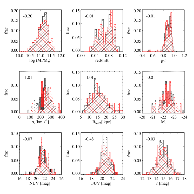
Figure 1: A comparison of the S1 BCGs with the control sample. We plot histograms of stellar mass, redshift, $g-r$ colour, galaxy velocity dispersion, R_iso23 radius, absolute r-band (AB) magnitude, and NUV and FUV apparent magnitudes. BCGs are in red and control galaxies are in black. In the top left-hand corner of each panel we list the logarithm of the Kolmogorov-Smirnov probability that the two distributions are drawn from an identical parent population (a 99 percent probability that the distributions are different will have a value of -2).

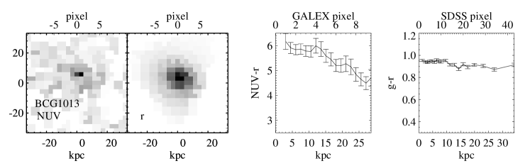
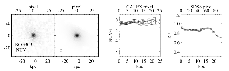
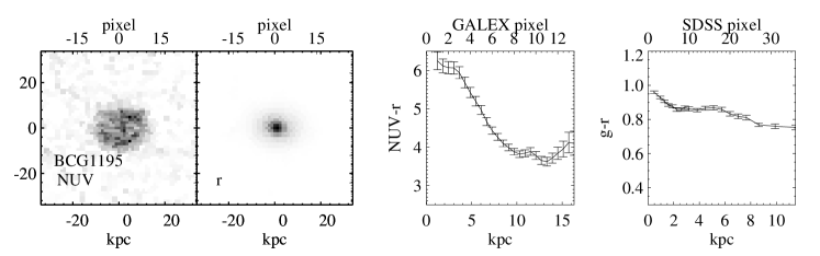
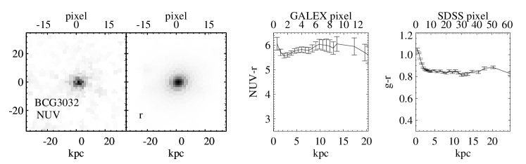
Figure 2: Some examples of typical BCGs in our dataset. The first row shows a typical BCG in our sample with low S$/$N in the UV, the second row a UV bright BCG with red colour and flat $NUV-r$ gradient, the third row a UV-bright BCG with a steep colour gradient, and the fourth row a BCG with a blue $NUV-r$ core.

2.4 X-ray BCGs from Rafferty et al. (2008)

X-ray data provides information about the thermodynamic state of the gas in clusters: by deprojecting the X-ray spectra extracted in elliptical annuli from X-ray images, one can derive gas temperatures and densities and thereby estimate gas cooling time-scales and entropy. Traditionally, those clusters with “central” (determined by the limiting resolution of images) cooling time-scales shorter than the age of the universe ($\sim$10 Gyr) have been classified as cooling flow clusters (Fabian, 1994). Recently, however, several studies (Cavagnolo et al., 2008a, b; Rafferty et al., 2008, C08, R08 respectively afterwards) have attempted to measure entropy and cooling times at smaller cluster-centric radii using higher resolution data from the Chandra satellite. These studies established a more stringent cooling time threshold of $\sim$1 Gyr (or 0.8 Gyr at a radius of 12 kpc from Rafferty et al. (2008)) below which BCGs were observed to have significantly enhanced star formation. In our study, we adopt the latter definition, and refer to clusters (and their associated BCGs) with central cooling times of less than 1 Gyr as cool-core clusters/BCGs, and those with central cooling times greater than 1 Gyr as non-cool-core clusters/BCGs, respectively.

To assess whether X-ray and optically selected BCGs differ, we make use of the sample of 46 BCGs in Rafferty et al. (2008) with X-ray data from Chandra. We search for optical images in SDSS DR7 and find 21 matches (11 of these have spectra ): 12 out of the 21 are in cool-core clusters and 9 are in non-cool-core clusters. In order to compare colors$\backslash$stellar populations to the optically selected BCGs, we need to further restrict the sample to lie at $z$$\leq$0.1 and have GALEX coverage, resulting in a total of only 9 clusters (3 non-cool-core and 6 cool-core) (see Table 1).

3 Photometry

To ensure that our photometric measurements are consistent across the different bands, we transform all our images to the same geometry and effective resolution so that our photometric measurements trace the same part of each galaxy at different wavelengths.

3.1 Registering the images

We first run SExtractor¹ on each image to get the celestial and pixel coordinates for sources in the images (Bertin &Arnouts, 1996). We then select the most compact sources in the NUV images and match them to the celestial coordinates of sources in the SDSS and FUV images. We run the GEOMAP/GEOTRAN² tasks in IRAF, with the pixel coordinate pairs as input to register every image to the frame geometry of the corresponding NUV image.

3.2 Convolving the images to a common PSF

We first need to obtain the PSF for each image. For SDSS images, we use the “$read\_PSF$” software³ and read out the PSF models for the five bands directly from the corresponding psField file. We transform these SDSS PSF models to a GALEX pixel scale of $1.^{\prime\prime}5$. In order to get the PSF model for the NUV and FUV images, we first select stars within a radius of 1200 pixels around the center of each image. After masking nearby sources, we fit a two-dimensional gaussian function to the stars. We cut out small stamps around each star and shift them so that every star is centered exactly on the center of the stamp. We add these stamps together and adopt the combined stack as the best PSF model for the frame. We check the PSF models by subtracting the stack from each of the input stars. Then we run the IMMATCH/PSFMATCH task in IRAF to obtain kernel functions that we use to convolve the higher resolution SDSS images to the resolution of the corresponding NUV images. Figure 2 shows examples of the registered and convolved images of 4 different S1 BCGs with different UV/optical colours. The resulting images are adaptively binned in two dimensions using the algorithm of Cappellari et al. (2003) so that all pixels have a signa-to-noise ratio ($S/N$) above a certain fixed value. The resulting images are then able to show the extended, low surface brightness regions of the sources. The color profiles are obtained by averaging the colors in a set of elliptical rings with increasing radius around the BCG center. The rings are chosen to that all all points along the profile have errors below a certain fixed value. The first row in Figure 2 shows a typical BCG in our sample with low S$/$N in the UV, the second row shows a UV-bright BCG with red colors and a flat $NUV-r$ profile, the third row shows a UV-bright BCG with a steep color profile, and the fourth line a BCG with a blue $NUV-r$ core.

In Figure 3, we plot the positional differences between the centroid of the BCG measured from the convolved SDSS and GALEX images. As can be seen, the centroids generally agree to better than $1^{\prime\prime}$, but in a few cases the offsets can be as large as 3 arcseconds. We have checked these images by eye and we find the largest offsets between the centroids can be caused by (1) SExtractor centroiding on regions of star formation, which are more prominent in UV light, (2) failure of SExtractor to deblend the BCG from nearby UV bright sources, or (3) low $S/N$ of the UV image. So it is important to use SDSS image decided position parameters for both GALEX UV and SDSS photometry to ensure consistency.

Figure 3: Differences between UV and R-band centroid positions (in GALEX pixel units) of the BCGs in our sample.

3.3 Two-zone photometric measurements

In order to assess whether the BCGs in our sample have colour gradients, we measure colours both inside and outside a fixed aperture for each object in our sample. Because the SDSS $r$ band images are of good quality and high $S/N$ ratio, we use them as the basis for our two-zone photometry. We first mask all sources except the BCG. We use SExtractor to determine the ellipticity and position angle from the $r$ band image (Bertin &Arnouts, 1996). These determine the shape and position angle of the apertures that we use. Following vdL07, we define the total magnitude of the BCG as the light contained within the radius where the $r$-band surface brightness equals $(23+10\log(1+z))$ mag arcsec^-2 (which we denote as $r_{iso23}$). All our photometry measurements are processed inside this aperture, which encloses most of the light. The reason why we measure the BCG magnitude within $r_{iso23}$ and do not attempt to measure a total magnitude, is because the surface brightness profiles of BCGs are complex and do not follow a simple de Vaucouleurs profile (Gonzalez et al., 2005). We define R₅₀ and R₉₀ as the radii enclosing 50% and 90% of the total flux of the galaxy evaluated within $r_{iso23}$. We measure the total UV and $r$-band flux inside R₅₀ (in), and between R₅₀ and R₉₀ (out). We compute colours within these two regions and and define the color difference, $\Delta(NUV-r)=(NUV-r)_{\mathrm{i}n}-(NUV-r)_{\mathrm{o}uts}$. We apply this definition to our UV/optical colour measurements, because it has higher $S/N$ than more traditional measures of colour gradient. We caution that in Sect. 3.5 we will use a different measure of colour gradient, because we are comparing directly with existing studies published in the literature.

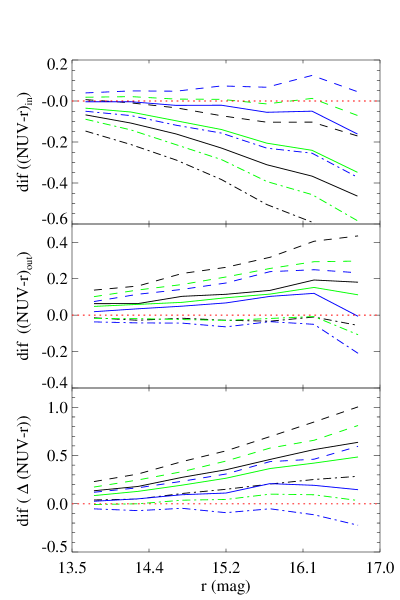
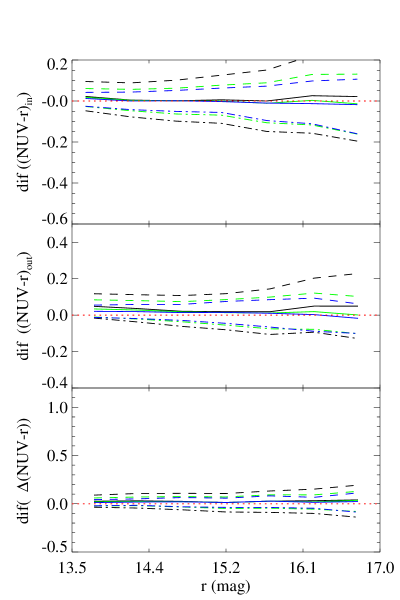
Figure 4: The results of tests using simulated images showing how the convolution procedure and sky noise will affect our colour measurements. The left column shows differences between the intrinsic (input) colours and the colours measured from the simulated images, which have been convolved to the resolution of the GALEX data and which have Poisson noise added. The right column shows the effect of just adding the Poisson noise. The data are divided into three different color bins ([5,5.5],[5.5,6],[6,6.5]) ( blue, green and black lines in the plot). Solid lines show the median values at a given $r$-band magnitude, while dashed lines show the $25\%$ and $75\%$ percentiles of the distribution at the same magnitude (see text for details).

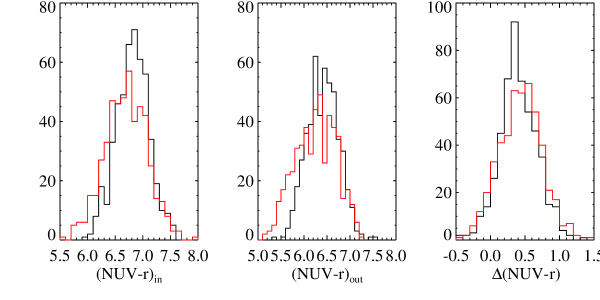
Figure 5: An analysis of the influence of structural parameter differences between BCGs and non-BCGs on our 2-zone color measurements (see text for details). Results are shown for simulated BCGs (red) and simulated non-BCGs (black). The simulated BCGs and non-BCGs have the same distribution of colours. The colour profiles of both kinds of objects are assumed to be flat. The differences between the red and black histograms arise purely because of the structural differences between the two classes of object.

3.4 Accuracy of our 2-zone color measurements

Recall that our two-zone photometry is carried out on optical images that have been convolved to the resolution of the GALEX data. It is thus important to understand to what extent our colour difference measurements reflect the intrinsic values for the real galaxy.

To assess this, we simulated 10,000 galaxies in the $r$ and NUV bands and included a similar level of background noise as in our real data (e.g. the MIS background for the simulated NUV images). The models assume Sersic profiles with $n$=4 for the $r$ band and $n$=2 for the UV band (i.e. we assume that the optical light comes from a bulge-like component and the UV from a star-forming disk). The range in $r$ magnitude, NUV magnitude and $r$-band effective radius for the simulated galaxies are constrained to be the same as in the vdL07 sample. By varying the effective radius of the NUV light, we obtain a set of simulated galaxies with different colour gradients. We then apply our algorithm to these images and compare our colour measurements to the intrinsic ”input” values in Figure 4. The inner color is defined to be the color inside R₅₀ and the outer color is defined as the colour between R₅₀ and R₉₀.

We begin by exploring the effect of noise of our colour measurements. The right column in Figure 4 shows the differences between the measured colours for model images with and without Poisson noise. The median value of the differences is zero across most of the $r$-magnitude range spanned by our BCG sample. Systematic effects only become important at $r$ magnitudes fainter than 16.1 (most of our BCGs are brighter than this). We then investigate what effect the convolution to GALEX resolution has on our measurements. The left column of the plot shows the measurement differences between model images with perfect resolution and the GALEX NUV resolution. The top panel shows that the inner $NUV-r$ colour will be underestimated and the situation is worse for redder objects. The middle panel shows that the outer $NUV-r$ colour will be over-estimated and the situation is again worse for redder objects. However, the outer color is better constrained in general than the inner colour. At an $r$-band magnitude of $\sim$16.0, the inner $NUV-r$ of the reddest objects will be underestimated by $\sim$0.3 mag, while that of the bluest ones would be underestimated by $\sim 0.1$ mag. The outer $NUV-r$ colour would be over-estimated by $\sim$0.15 mag on average. The bottom panel shows that the resulting color difference $\Delta(NUV-r)$ will be over-estimated by $\sim$0.5 mag at $r\sim$16.0. These results are easily understood from the fact that the optical light (with Sersic model $n$=4) is more concentrated than the UV light (with Sersic model $n$=2), and will thus be more severely scattered to the outer region of the galaxy. As we will show later on, our results are not substantially affected by these systematics.

Von der Linden et al.(2007) found that BCGs have larger effective radii and lower surface brightnesses than non-BCGs. We simulated two sets of galaxies with structural parameters similar to the optical BCGs and the control sample to check the extent to which differences in structural parameters affect our measurements of 2-zone colors. We fix the $r$ band magnitude to be 15 ($\sim$ median value of the optical sample), $NUV-r$ to be 6.0 (a typical value at the red end of our sample) and $\Delta(NUV-r)$ to be 0. Only the mean surface brightness inside $R_{50}$, $\mu_{50}$, is allowed to vary ($R_{50}$ will vary accordingly since the total $r$ magnitude is fixed). The median values of $\mu_{50}$ are fixed to be 18.82 and 18.65 mag for BCGs and non-BCGs respectively (corresponding to the median values of the two samples as measured by vdL07). $\mu_{50}$ is allowed to vary randomly around the median value with a scatter of 0.7 mag arcsec^-2 (again according to von der Linden’s distribution). We compare the distributions of the values of $(NUV-r)_{\mathrm{i}n}$, $(NUV-r)_{\mathrm{o}ut}$, and $\Delta(NUV-r)$ (defined as in Sect 3.3) for BCGs (red) and non-BCGs (black) in Figure 5. It can be seen that structural differences cause both the inner and outer colours of BCGs to be shift slightly bluewards relative to non-BCGs. However, the color differences for the two samples are similar. We have also simulated cases where the input galaxies have an intrinsic colour gradient, and the results are similar.

3.5 $u-r$ gradients

The SDSS optical photometry is of higher resolution than the GALEX photometry, so $u-r$ colour gradients offer an alternative way to trace star formation in the central regions of early type galaxies. As was found by R08 and will be seen in Sect 4.3, X-ray selected cool-core BCGs have steeper $u-r$ colour gradients than non-cool-core BCGs. We will use $u-r$ gradients to link our study of optical selected BCGs to previous studies of X-ray selected BCGs (e.g. R08).

We use the SDSS $r$ and $u$ band images to measure the $u-r$ colour profiles. These images have lower resolution and poorer seeing than the images used by R08, but we produce high quality color profiles by registering and convolving the $u$ band images to the $r$ band images. We then measure the color gradients ($G(u-r)$) following the procedures oulines in in R08.

The procedure we employ is the following. We measure colours in a series of elliptical annuli, with the major axis increasing in $\sim$ 1 pixel intervals. If the $u-r$ profile has a positive color gradients near the center that extends for more than 4 sampling intervals ($\sim$ 2.2 arcsec) from a point near the center of the galaxy at twice the FWHM of the PSF, the galaxy is classified as having a blue core. The blue core region is defined to end where the colour gradients become negative. Otherwise, the galaxy is classified as having a red core. We fit the colour profile in the radius range from twice the FWHM of the PSF to where the excess blue emission ends (for objects with blue cores) or where the total errors reach 0.5 mag (for objects with red cores), and define the colour gradient $G(u-r)$ as the slope of the fit. Figure 6 shows the $u-r$ profiles and the range of our adopted linear fits for two BCGs from the R08 X-ray sample.

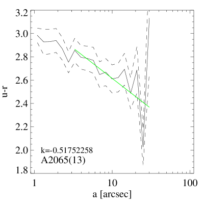
Figure 6: $u-r$ differential color profiles of two BCGs from the R08 X-ray sample (A1795 and A2065). The dashed lines show the 1 $\sigma$ range of the profile. The best-fit gradients are overplotted as green straight lines in the fitting ranges as defined in Sect. 3.5. The values of the best-fit gradients are shown in the left-down corner of each profile.

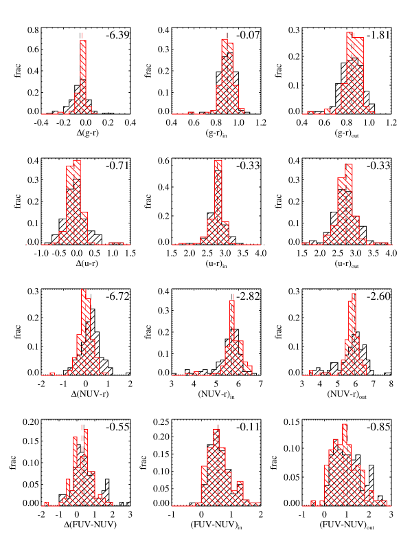
Figure 7: Distribution of 2-zone colours and colour differences for optical BCGs (red) and the control sample of massive field galaxies (black). The dashed lines mark the median values for the two distributions.

4 results

4.1 BCGs and control galaxies

In Figure 7, we compare the normalized distribution of colours and colour differences for S1 BCGs (red) (see definition in Sect 2.2) and control galaxies (black). Colours are measured in two zones: inside $R_{50}$ (denoted by $colour_{\mathrm{i}n}$) and between $R_{50}$ and $R_{90}$ (denoted by $colour_{\mathrm{o}ut}$). Colour differences here follow the definition in Sect 2. The results of a Kolmogorov-Smirnov test (specifically, the logarithm of the K-S probability that the two distributions are drawn from an identical parent population) are given in each panel. Smaller values mean larger differences between the two distributions (a 99 percent probability that the distributions are different will have a value of -2). Dashed lines in each panel indicate the median values of the distributions.

The top two panels show SDSS colours measured for the BCGs and control galaxies. There is no systematic difference in median colour between the two samples. However, non-BCGs clearly have larger scatter in their colours than BCGs, particularly in their outer regions. This translates into a broader range in colour differences, which is consistent with the conclusions of vdL07, who found that BCGs have more homogeneous stellar populations than non-BCGs.

There are clear systematic shifts in the $NUV-r$ colours of BCGs and non-BCGs in the sense that BCGs have bluer outer $NUV-r$ colours and redder inner $NUV-r$ colours. The first question one might ask is whether these shifts are real, or whether they simply reflect that fact that BCGs have larger sizes ($R_{50}$) and lower optical surface brightness than non-BCGs. As discussed in Sect. 3.4, this may indeed partly explain why BCGs have bluer outer $NUV-r$ colours. Using the colour distributions of our sample of BCGs and non-BCGs, we estimate that the net shift due to structural differences between the two kinds of galaxies is about 0.1 mag, and thus cannot explain the differences between the two distributions (the reddest non-BCGs are $\sim$0.4 mag redder than the BCGs). Also, we find that the inner $NUV-r$ colours of BCGs are redder than those of non-BCGs, which goes in the opposite direction to the effect predicted from the simulations In summary, our result that BCGs have bluer outer $NUV-r$ colours than non-BCGs may be weaker than suggested in Figure 7, but the result that BCGs have redder inner $NUV-r$ colours than non-BCGs is robust. This would imply that the inner stellar populations of BCGs are older, more metal rich, or more dusty (or some combination of these).

We find no detectable differences in the $FUV-NUV$ colours of BCGs and non-BCGs. This may be due to lower quality of the FUV images.

We note that the BCGs and comparison galaxies have been matched in redshift, so $K$-corrections are not an issue in our analysis. Finally, as discussed in Sect 2.3, the control galaxies correpsonding to BCGs in less massive clusters may be ”contaminated” with BCGs. We have checked whether there is any trend in the differences betweeen the colours of BCGs and non-BCGs as a function of cluster mass, but we did not find any effect.

4.2 Optical BCGs versus X-ray BCGs

Figure 8 shows the distributions of $\sigma_{cluster}$ and X-ray luminosity (when it is available from ROSAT, Shen et al. (2008)) for the vdL07 sample. In the following analysis, we limit the optical BCG sample to those objects in clusters with $\log{\sigma_{cluster}}>2.8$ km s^-1. After including galaxies with GALEX AIS photometry, the sample consists of 60 BCGs. The X-ray selected BCGs from R08 (Table 1) are still significantly biased towards higher $\sigma_{cluster}$ and even more severely towards higher X-ray luminosities compared to the optically-selected clusters. We will come back to this point later in our discussion.

Figure 9 plots the BCGs at z$\leq$0.1 in a series of colour/magnitude and colour/colour diagrams. BCGs in optically-selected clusters are shown as black points and BCGs in X-ray selected clusters are shown as coloured symbols (cool-core BCGs in green and non-cool-core BCGs in red). Most X-ray selected BCGs have high $r$-band luminosities compared to the optical BCGs. X-ray selected BCGs have similar $g-r$ and $u-r$ colours to the optically selected BCGs, but blue inner NUV–r colours. Among the X-ray selected BCGs, the cool-core BCGs are always bluer than the non-cool-core ones (cool-core and non-cool-core BCGs separate at a $NUV-r$ colour of $\sim$5.8). This demonstrates that the UV and optical colours of the X-ray selected BCGs are indeed correlated with the cooling time of the gas. One of the objects with the bluest $NUV-r$ colour is the BCG in the well studied very strong cooling flow cluster A1795 (O’Dea et al., 2004; Mittaz et al., 2001). The other blue outlier is M87, which is an AGN. The synchrotron emission from its jet is quite prominent in the UV (Madrid et al., 2007).

In Table 2, we list K-S test probabilities for colour differences between optically and X-ray selected BCGs, as well as optically selected BCGs and cool-core BCGs. The results confirm our assertion that the most significant differences are found for UV/optical colours and for optically-selected and cool-core BCGs. Could the large differences in UV/optical colours be an artifact of our convolution algorithm? As discussed in Sect 3.4, the inner $NUV-r$ colours are more severely underestimated for red objects than for blue objects. So if we were to correct our colour measurements to the value before convolution, red galaxies will become redder in $NUV-r$ while blue galaxies will not change much. In other words, the $NUV-r$ colour differences between the cool-core and non-cool-core BCGs would be enhanced even more.

Number	Name	Redshift	$\sigma_{cluster}$	LX	H$\alpha$	tcool	G(u-r)R08	G(u-r)
			(km s-1)	(1044 ergs-1)	(1040 erg s-1)	(108 yr)
1	A85	0.055	1097w	16.5w	0.502	6.4	$0.02\pm 0.04$	$0.244\pm 0.230$
2	A383	0.187	920w	9.8s	–	4.4	$0.15\pm 0.28$	$-0.248\pm 2.120$
3	Perseus	0.018	925w	19.7w	–	5.5	–	$0.568\pm 0.010$
4	A1361	0.117	–	3.22e	13.5c	8	$-0.15\pm 0.06$	$-0.403\pm 0.131$
5	A1413	0.143	1231w	16.6w	0	15	$-0.29\pm 0.15$	$-0.534\pm 0.316$
6	M87	0.004	350w	0.66w	–	8.6	$-0.27\pm 0.08$	$-0.068\pm 0.004$
7	A1650	0.084	1033w	7.01w	–	15.5	$-0.14\pm 0.11$	$-0.063\pm 0.064$
8	Coma	0.023	1010w	9.14w	0.0298	71.8	$-0.14\pm 0.02$	$0.018\pm 0.016$
9	A1795	0.063	920w	20.1w	11.3c	7.2	$0.5\pm 0.1$	$0.777\pm 0.072$
10	A1991	0.059	720w	3.29w	1.1c	4.1	$-0.35\pm 0.06$	$-0.134\pm 0.052$
11	MS1455.0+2232	0.258	964H	10.51eg	1.816	3.9	$-0.06\pm 0.23$	$-0.557\pm 1.271$
12	RXCJ1504.1-0248	0.215	–	28.07b	475.595	2.9	$0.94\pm 0.17$	$1.443\pm 0.280$
13	A2065	0.073	908w	3.88w	–	15	$-0.38\pm 0.08$	$-0.518\pm 0.132$
14	RXJ1532.8+3021	0.354	–	32.9h	415c	3.7	$1.04\pm 0.4$	$0.209\pm 0.532$
15	A2244	0.097	930p	6.6p	0.333	17.4	$-0.2\pm 0.12$	$0.278\pm 0.161$
16	NGC6338	0.027	–	43.28H1	0.909	9	–	$0.001\pm 0.017$
17	RXJ1720.2+2637	0.164	–	25.58h	12.7c	5.3	$0.28\pm 0.14$	$0.924\pm 0.344$
18	MACSJ1720.2+3536	0.391	–	–	–	3.6	$0.84\pm 0.85$	–
19	A2261	0.224	–	18.06e	1.318	9.3	$-0.42\pm 0.19$	$-0.578\pm 1.194$
20	A2409	0.148	–	8.04e	0c	23.7	$-0.34\pm 0.26$	$-1.705\pm 1.646$
21	A2670	0.076	908w	3.88w	0.1c	23.4	–	$-0.694\pm 0.085$

Table 1: Properties of the BCGs in the X-ray selected sample of (R08). Columns 2 and 3 list the velocity dispersions and X-ray luminosities of the host clusters, which have been obtained from a variety of different sources as indicated by a superscript to the values of $L_{X}$ as follows: $s$ refers to Smith et al. (2001), $e$ refers to Ebeling et al. (1996), $eg$ refers to Egami et al. (2006), $h$ refers to Hashimoto et al. (2007), $H$ refers to Hoekstra et al. (2007), $H1$ refers to Helsdon et al. (2001) , $p$ refers to Peres et al. (1998), $w$ refers to D.A.White et al. (1997). Column 4 lists the H$\alpha$ emission line luminosities of the BCGs. $c$ means the H$\alpha$ luminosity comes from Crawford et al. (1999), otherwise it is from SDSS DR4. Column 5 is the cooling time of the gas calculated by R08. Column 6 lists the $u-r$ colour gradient given by R08, while Column 7 is our own measurement of the same quantity using imaging data from SDSS

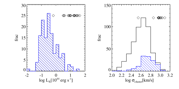
Figure 8: $\sigma_{cluster}$ (right panel) and X-ray luminosity (left panel) of the entire optical BCG sample (black) and subset of the optically-selected BCGs with data from ROSAT (blue). The diamonds mark the values of the X-ray selected R08 BCGs used in this work.

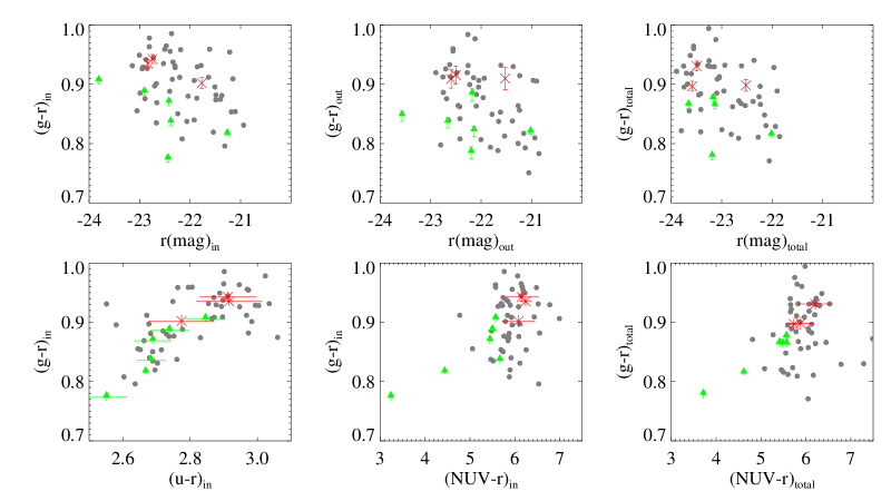
Figure 9: Comparison between the inner and outer colours of optical BCGs (black, filled circles; only those in clusters with $\sigma_{v}>$2.8 are plotted), cool-core (green, filled triangle) and non-cool-core BCGs (red, crosses).

	Mr	(g–r)total	(g–r)in	(u–r)total	(u–r)in	(NUV–r)total	(NUV–r)in
X-ray vs optical	-0.26	-0.32	-0.66	-0.58	-0.21	-1.55	-1.39
cool-core vs optical	-0.60	-1.49	-1.26	-0.22	-0.94	-3.69	-3.51

Table 2: K-S test values (the logarithm of the K-S probability that the two distributions are drawn from an identical parent population) for differences between optically selected BCGs, X-ray selected BCGs and cool-core X-ray BCGs. It shows that the difference of $(NUV-r)_{in}$ between X-ray selected (especially cool-core) and optical selected BCGs is strong.

4.3 Consistency with previous work

In the previous subsection, we showed that cool-core and non-cool-core clusters segregated rather cleanly in colour space, implying that the presence of young stars in the BCG is related to the cooling time of the gas in cluster cores.

There have been a number of studies of X-ray selected clusters that have found that there is a central entropy (or t_cool) threshold below which BCGs have significant H$\alpha$ line emission and blue cores (Bildfell et al., 2007; Rafferty et al., 2008; Pipino et al., 2008; Cavagnolo et al., 2008a).

We now check whether we reproduce these results using the sample of X-ray BCGs from R08. For this analysis, we do not impose a cut on the sample at $z\leq$0.1 – the reason is that this would reduce the sample size by too much. Table 1 shows the values of the $u-r$ colour gradients given in R08 and our measurements from the SDSS images. The measurements are generally consistent given the uncertainties. When available, we take the H$\alpha$ fluxes from Crawford et al. (1999) (to be consistent with Cavagnolo et al. (2008a)), otherwise, we adopt the H$\alpha$ fluxes in the SDSS DR7 emission line catalog released by the MPA/JHU group.

We plot $u-r$ colour and H$\alpha$ luminosity versus t_cool in Figures 10 and  11 respectively. We use the cross correlation parameter $\rho=\langle(X-\bar{X})(Y-\bar{Y})\rangle$ to evaluate the significance of corrleation between parameter $X$ and $Y$. As can be seen, we do verify a threshold $t_{cool}$ value of $\sim$1 Gyr below which some BCGs exhibit significant H$\alpha$ luminosity and blue cores. It should be noted, however, that not all BCGs with $t_{cool}<1$ Gyr are strongly star-forming. There is a significant scatter in H$\alpha$ luminosity and colour gradient values and only weak correlation with the actual value of $t_{cool}$ below the threshhold value. If we plot $u-r$ colour gradient versus H$\alpha$ luminosity for these X-ray BCGs (Figure 12), there is a significant correlation between the two quantities (albeit with large scatter). We also find similar correlations between $u-r$ colour differences (following the definition from R08) and both H$\alpha$ luminosity and H$\alpha$ equivalent width.

We note that the scatter may arise because H$\alpha$ line emission is produced by ionizing photons from massive stars with lifetimes of $\sim 10^{7}$ years, whereas the $u-r$ colour gradients will be sensitive to star formation that has taken place over Gyr timescales. In addition, it is possible that part of the H$\alpha$ line emission does not originate from HII regions, but is excited by a central AGN.

We have also checked whether there is a correlation between $u-r$ colour gradient and H$\alpha$ luminosity in the ROSAT (top) and GALEX MIS (bottom) detected sample of optically-selected BCGs from vdL07 and the results are shown in Figure 13; the lower redshift range of $z<0.1$ ensures that the $u-r$ colour gradients can be measured relatively accurately. In the top panel, the points are colour-coded according to the total X-ray luminosity of the cluster (clusters with ROSAT X-ray luminosities greater than $10^{43.5}$ erg s^-1 are plotted in red). In the bottom panel, the points are coded according to the $NUV-r$ colour of the BCG. We fail to find any correlation between colour gradients and H$\alpha$ luminosity for any of the subsamples defined from the optically-selected clusters.

This may not be too surprising in view of the fact that the optically selected BCGs span a much smaller range in H$\alpha$ luminosity. (most L${}_{H\alpha}<$1.1$\times 10^{40}$ erg/s). Much of the correlation seen in Figure 12 is driven by the BCGs with the very higher H$\alpha$ luminosities. Over the range in H$\alpha$ lumnosity where the R08 sample overlaps the optically selected clusters, the results are actually in fairly good agreement.

Figure 10: The $u-r$ colour gradient as defined in R08 (bottom, see text) is plotted as a function of the cooling time of the gas in units of $10^{8}$ years. The dashed line marks 0.8 Gyr, which R08 claim to be the threshold for finding blue cores. Numbers are used to mark individual BCGs as listed in Table 1. $\rho$ is the cross correlation parameter, as defined in Section 4.3. .

Figure 11: $H\alpha$ line luminosity is plotted against $t_{cool}$ for the R08 BCG sample. Numbers are used to mark individual BCGs. $\rho$ is the cross correlation parameter.

Figure 12: The correlation between $G(u-r)$ and $H\alpha$ line luminosities for the R08 sample. Numbers are used to mark individual BCGs. $\rho$ is the cross correlation parameter.

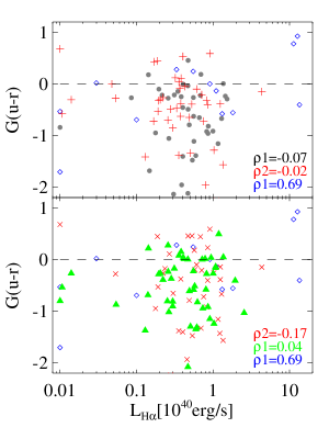
Figure 13: The correlation between $G(u-r)$ and $H\alpha$ line luminosities for the optically selected BCG of vdL07. In the bottom panel, the BCGs with $NUV-r<$5.8 are in green (filled triangles), and others are in red (crosses). In the top panel, the BCGs with ROSAT X-ray luminosities $>10^{43.5}$ erg s^-1 are in red (pluses), otherwise they are in grey (solid points). Blue points (diamonds) indicate R08 BCGs. $\rho$ is the cross correlation parameter for the symbols of corresponding colour.

5 Summary and Discussion

The main aim of this paper is to investigate the claim that the bright galaxy located at the center of a massive dark matter halo (BCG) forms stars at a higher rate than galaxies of similar mass and structure that are not located at cluster or group centres. Studies of BCGs from X-ray selected cluster samples have generally supported this claim. Anlayses of BCGs from optically-selected cluster samples have failed to find any significant enhancement in star formation when compared to control samples of non-BCGs.

Recent work on optically-selected BCGs relied on spectroscopic indicators derived from Sloan Digital Sky Survey spectra. This has the disadvantage of only probing the most recent star formation that is occurring in the cores of the BCGs. In this paper, we analyzed a sample of 113 BCGs with $z<0.1$ with optical imaging from SDSS and UV data from GALEX. We convolved the SDSS images to match the resolution of the GALEX data and measured UV/optical colours both in the inner and outer regions of the BCGs. We did the same for a smaller sample of X-ray selected BCGs with gas cooling times derived from Chandra data.

Our main conclusions concerning our sample of optically-selected BCGs are the following:

1. We confirm the conclusion of vdL07 that optically-selected BCGs have similar median $g-r$ and $u-r$ colours as control samples of non-BCGs with the same stellar mass and concentration. This conclusion holds for colours measured in both the inner and the outer regions of the galaxies.

2. Optically-selected BCGs have smaller scatter in their $g-r$ and $u-r$ colours than the control non-BCGs.

3. Optically-selected BCGs have slighly redder $NUV-r$ colours in their centres than the control galaxies.

4. Correlations between $G(u-r)$ and $H\alpha$ luminosity are very weak.

Taken together, the three findings lead us to conclude that optically-selected BCGs are slightly older and have had less recent star formation than the galaxies in the control sample.

Our main conclusions concerning our sample of X-ray BCGs are the following:

1. The optical ($g-r$ and $u-r$) colours of the BCGs in the X-ray selected cluster sample span a similar range as those in the subset of optical clusters with high cluster ($\log\sigma>2.8$) velocity dispersions. Their $NUV-r$ colours, on the other hand, are significantly bluer.

2. Among the X-ray selected BCGs, those that are located in the centre of a cool-core cluster (defined to have central cooling times of less than 1 Gyr) always have bluer optical and UV/optical colours than those that are located in clusters where the central gas cooling times are long.

3. We confirm that there appears to be a threshold value of the central cooling time below which star formation does occur in a subset of clusters.

Our main conclusion, therefore, is that the location of a galaxy at the center of a dark matter halo is not sufficient to determine whether or not it is currently forming stars – one must also have information about the thermo-dynamic state of the gas in the core of the dark matter halo. These results agree with other similar studies. Egami et al. (2006) found that the majority of the BCGs are not particularly infrared-luminous compared with other massive early-type galaxies. Edward et al. (2007) found their red BCGs selected from the SDSS sample had a low fraction with emission lines ($11\pm 2$ percent), comparable to that found in their control sample However, both papers noted that for BCGs in clusters where cooling times are very short and the predicted cooling flow rates are high, star formation is prominently enhanced.

Perhaps the most important lesson to take away from this analysis, is that BCGs selected from optical cluster surveys and BCGs selected from X-ray cluster surveys will be different. Low redshift spectroscopic surveys such as the SDSS are designed to provide a complete census of the most massive galaxies out to redshifts of $0.2-0.3$. The fact that only a relatively small percentage of BCGs in these surveys have signs of recent star formation must indicate that the majority of nearby BCGs do not sit at the centers of dark matter halos in which central cooling time of the gas is less than 1 Gyr. As shown by Best et al. (2007), a large fraction (20-30%) of optically-selected BCGs host radio-loud AGN, which may play a key role in preventing the gas from cooling.

It remains to be seen whether the same conclusion will hold up at higher redshifts. Many of the most strongly star-forming BCGs in the current X-ray samples are located at relatively high redshifts. We checked the full R08 sample and found that the ratio of blue core BCGs to those with negative gradients increases with redshift: 19:27 for the whole sample, 13:8 for BCGs at $z>$0.1, and 6:3 for BCGs at $z>$0.2. In addition, Crawford et al. (1999) found that the fraction of emission line BCGs increases with redshift. We note that the cluster sample of vdL07 is defined to lie at redshifts below 0.1, so this may explain why the BCGs in this sample are predominantly inactive. On the other hand, only the most X-ray luminous clusters can currently be detected at higher redshifts and these are likely to be biased to systems with short central cooling times. A new generation of both optical spectroscopic surveys (e.g. SDSS-III’s Baryon Oscillation Spectroscopic Survey ($BOSS$)) and deeper X-ray imaging surveys over large areas of the sky (e.g. the extended Röentgen Survey with an Imaging Telescope Array (eROSITA) will be needed before these issues can be fully understood.

References

- Allen (1995) Allen, S.W., 1995, MNRAS, 276,947
- Babul et al. (2002) Babul, A., Balogh, M.L., Lewis, G.R., Poole,G.B., 2002,MNRAS, 330,329
- Bauer et al. (2005) Bauer, F.E., Fabian, A.C., Sanders, J.S., Allen, S.W., &Johnstone, R.M., 2005, MNRAS, 359,1481
- Best et al. (2007) Best P. N., von der Linden A., Kauffmann G., Heckman T. M., Kaiser C. R., 2007, MNRAS, 379, 894
- Bernardi et al. (2007) Bernardi, Mariangela, Hyde, Joseph, Sheth, Ravi, Miller, Chris , &Nichol, Robert, 2007, AJ, 133,1741
- Bertin &Arnouts (1996) Bertin, E., Arnouts, S., 1996, A&AS, 117,393
- Bildfell et al. (2007) Bildfell, Chris, Hoekstra, Henk, Babul, Arif, &Mahdavi, Andisheh, 2007, MNRAS, 000, 1
- Biviano et al. (2006) Biviano, A., Murante, G., Borgan, S., Diaferio, A., Dolag, K., &Girardi, M., 2006, A&A, 456, 23
- Böhringer et al. (2004) Böhringer, H., Schuecker, P., et al., 2004, A&A, 425, 367
- Bruzual &Charlot (2003) Bruzual, G, Charlot, S., 2003, MNRAS, 344,1000
- Cappellari et al. (2003) Cappellari, Michele, & Yannick, Copin, 2003, MNRAS, 342, 345
- Cardiel et al. (1995) Cardiel, N, Gorgas, J., &Aragón-Salamanca, A., 1995, MNRAS, 277,502
- Cavagnolo et al. (2008a) Cavagnolo, Kenneth, Donahue, Megan, Voit, G., &Sun, Ming, 2008, ApJ, 683,107
- Cavagnolo et al. (2008b) Cavagnolo, Kenneth, Donahue, Megan, Voit, G., &Sun, Ming, 2008, ApJ, 682, 821
- Charlot &Fall (2000) Charlot, S., &Fall, S., 2000, ApJ, 539,718
- Crawford et al. (1999) Crawford, C.S., Allen, S.W., Ebeling, H., Edge, A.C., &Fabian, A.C., 1999, MNRAS, 306, 857
- Blanton et al. (2003) Blanton, Elizabeth, Sarazin, Craig, &McNamara, Brian, 2003, ApJ, 585:227
- Desroches et al. (2007) Desroches, Louis-Benoit, Quataert, Eliot, Ma, Chung-Pei, &West, A.A., 2007, MNRAS, 377,402
- Donahue et al. (2007a) Donahue, Megan, &Sun, Ming, 2007, ApJ, 670,231
- Donahue et al. (2007b) Donahue, Megan et al., 2007, AJ, 134,14
- Ebeling et al. (1996) Ebeling, H., Voges, W. et al. 1996, MNRAS, 283,1103
- Edge (1997) Edge, A.C., 1997, ASP conference Serises, 115, 1997
- Edward et al. (2007) Edwards, Louise, Hudson, Michael, Balogh, Michael, &Smith, Russell, 2007, MNRAS, 397,100
- Egami et al. (2006) Egami, E. et al., 2006, ApJ, 647,922
- Fabian (1994) Fabian, A.C., 1994, ARA&A, 32,277
- Gonzalez et al. (2003) Gonzalez, A.H., Zabludoff, A.I., &Zaritsky, Dennis, 2003, Ap&SS, 285,67
- Gonzalez et al. (2005) Gonzalez, A.H., Zabludoff, A.I., &Zaritsky, Dennis, 2005, ApJ, 618, 195
- Hashimoto et al. (2007) Hashimoto, Y., Böhringer, H., et al., 2007, A&A, 467, 485
- Helsdon et al. (2001) Helsdon, S. F., Ponman, T. J., et al., 2001, MNRAS, 325, 613
- Hicks et al. (2005) Hicks, A.K., &Mushotzky, R., 2005, ApJ, 635,9
- Hoekstra et al. (2007) Hoekstra, Henk, 2007, MNRAS, 379, 317
- James et al. (2006) James, P.A., Salaris, M., Davies, J.I., Phillipps, S., Cassisi, S., 2006, MNRAS, 367,339
- Kauffmann et al. (2003) Kauffmann, G. et al. 2003, MNRAS, 341,54
- Kuchinski et al. (2008) Kuchinski, L.E., Freedman, W.L., Madore, B.F. et al. 2000, ApJS, 131, 441
- von der Linden et al. (2007) von der Linden, Anja, Best, Philip, Kauffmann, Guinevere, &White, Simon, 2007, MNRAS, 379,893
- Liu et al. (2008) Liu, F.S, Xia, X.Y, Mao, Shude ,Wu, Hong, &Deng, Z.G, 2008, MNRAS, 385,23
- López-Gruz et al. (1997) López-Gruz, Omar, Yee, H.K., Brown, James, Jones, Christine, &Forman, William, 1997, ApJ, 475,97
- Lucia et al. (2007) Lucia, G.De, &Blaizot, Jérémy, 2007, MNRAS, 375,2
- Madrid et al. (2007) Madrid, Juan P., Sparks, William B., Harris, D. E., Perlman, Eric S., Macchetto, Duccio, & Biretta, John, 2007, Ap&SS, 311, 2
- Martin et al. (2005) Martin, D.C.,and the GALEX Team., 2005, ApJ,619,L1
- McCarthy et al. (2004) McCarthy, I.G., Balogh, M.L., Babul, A., Poole, G.B., Horner, D.J., 2004, ApJ, 466,L9
- Miller et al. (2005) Miller, C.J. et al., 2005, AJ, 130,968
- Mittaz et al. (2001) Mittaz, J.P., Kaastra, J.S., Fabian, A.C., Mushotzky, R.F., Peterson, J.R., Ikebe, Y., Lumb, D.H., Paerels, F., Stewart, G., &Trudolyubov, S., 2001, A&A, 365,93
- Murante et al. (2004) Murante, G. et al., 2004, ApJ, 607,83
- O’Dea et al. (2004) O’Dea, Christopher, Baum, Stefi, Mack, Jennifer, &Koekemoer, Anton, 2004, ApJ, 612, 131
- O’Dea et al. (2008) O’Dea, Christopher, Baum, Stefi, Privon, George, &Jacob, Noel-Storr, 2008, ApJ, 681, 1035
- Peres et al. (1998) Peres, C.B., Fabian, A.C., Edge, A.C., Allen, S.W., Johnstone, R.M., &White, D.M., 1998, MNRAS, 298,416
- Pipino et al. (2008) Pipino, A., Kaviraj, S., Bildfell, C., Hoekstra, H., Babul, A., &Silk, J., 2008, MNRAS, 000,1
- Rafferty et al. (2008) Rafferty, D.A., McNamara, B.R., &Nulsen, P.E.J., 2008, accepted for publication in ApJ,
- Rudick (2006) Rudick, Craig, Mihos, J., &McBride, Cameron, 2006, ApJ, 648,936
- Salpeter (1955) Salpeter,E.E., 1955, ApJ, 121, 161
- Shen et al. (2008) Shen, Shiyin, Kauffmann, Guinevere, von der Linen, Anja, White, Simon D. M., & Best, P.N., 2008, MNRAS, 389, 1074S
- Smith et al. (2001) Smith, G.P., Kneib, Jean-Paul, et al., 2001, AJ, 552, 493
- Tegmark et al. (2004) Tegmark, M., Strauss, M.A., Blanton, M.R. et al., 2004, Phys. Rev. D, 69, 103501
- York et al. (2000) York, D. G. et al., 2000,AJ,120,1579
- Voit et al. (2008) Voit, G., Cavagnolo, K., Donahue, M., Rafferty, D., McNamara, B., &Nulsen, P., 2008, ApJ, 681,5
- R.E.White et al. (1988) White,R.E., & Sarazin, C.L., 1988, ApJ,335,688W
- D.A.White et al. (1997) White, D.A., Jones, C., Forman, W., 1997, MNRAS, 292,419