30 GHz observations of sources in the VSA fields

Abstract

Small angular scale (high $\ell$) studies of cosmic microwave background anisotropies require accurate knowledge of the statistical properties of extragalactic sources at cm-mm wavelengths. We have used a 30 GHz dual-beam receiver (OCRA-p) on the Toruń 32-m telescope to measure the flux densities of 121 sources in VSA fields selected at 15 GHz with the Ryle Telescope. We have detected 57 sources above a limiting flux density of 5 mJy, of which 31 sources have a flux density greater than 10 mJy, which is our effective completeness limit. From these measurements we derive a surface density of sources above 10 mJy at 30 GHz of $2.0~{}\pm~{}0.4$ per square degree. This is consistent with the surface density obtained by Mason et al. (2009) who observed a large sample of sources selected at a much lower frequency (1.4 GHz). We have also investigated the dependence of the spectral index distribution on flux density by comparing our results with those for sources above 1 Jy selected from the WMAP 22 GHz catalogue. We conclude that the proportion of steep spectrum sources increases with decreasing flux density, qualitatively consistent with the predictions of de Zotti et al. (2005). We find no evidence for an unexpected population of sources whose spectra rise towards high frequencies, which would affect our ability to interpret current high resolution CMB observations at 30 GHz and above.

1 Introduction

Extragalactic radio sources are a serious contaminant in observations of primordial Cosmic Microwave Background (CMB) anisotropies on small angular scales (high $l$; e.g. Toffolatti et al., 2005). In order to estimate the CMB temperature power spectrum with high accuracy, detailed information about the foreground population is required. CMB experiments can be designed to work at any of a range of frequencies from $\sim$20 to $\sim$300 GHz, since the spectrum peaks at $\sim 160$ GHz. Extragalactic radio sources are problematic over most of this range, with different source populations, from active galaxies to star-forming galaxies, dominating the contamination in different wavebands. However, information on these contaminating populations is limited, since large-scale high-resolution surveys of the radio sky are restricted to lower frequencies, as for example in the NRAO VLA Sky Survey (NVSS; Condon et al., 1998) at 1.4 GHz and the Green Bank 4.85 GHz survey (GB6; Gregory et al., 1996). Model-dependent predictions of the contaminating sources at the frequencies of CMB experiments may be made (e.g. Toffolatti et al., 1998; de Zotti et al., 2005), but these can be unreliable. Source populations can exhibit a wide range of spectral indices so that severe selection effects may arise when extrapolating to high frequencies from the limited set of surveys on which these predictions are based. Thus, for maximum reliability in their cosmological interpretation, it is essential that CMB observations are complemented by deep and carefully-selected high-frequency radio source surveys.

The CMB power spectrum has been measured over a wide range of angular scales, from the early low-resolution (7^∘ per beam) work of the Cosmic Background Explorer (COBE, Smoot et al., 1992), through the intermediate scales probed by e.g. the Very Small Array (VSA, see e.g. Dickinson et al. 2004), Boomerang (see e.g. Jones et al., 2006) and the Wilkinson Microwave Anisotropy Probe (WMAP, see e.g. Hinshaw et al., 2003, 2009), up to the high resolution measurements of e.g. the Cosmic Background Imager (CBI, see e.g. Sievers et al., 2009) and the Arcminute Cosmology Bolometer Receiver Array (ACBAR, see e.g. Reichardt et al., 2009). The problem of contamination by radio sources increases at high multipole order, $\ell$, since the power spectrum of point sources increases as $\ell^{2}$. Source subtraction strategies are therefore becoming ever more important. This is particularly so because of the results obtained with the CBI at 30 GHz, which indicate an excess of power at high $\ell$ compared to best fit cosmological models, the so-called ‘CBI excess’ (Mason et al., 2003; Readhead et al., 2004; Sievers et al., 2009). There has been much discussion of this result with some new observations not detecting a significant excess of power at $\ell>2000$ (Sharp et al., 2009; Friedman et al., 2009; Reichardt et al., 2009), though most either do not cover the same range of multipoles or are at different observing frequencies.

One possibility is that the excess arises from a population of point sources, another is that that the power comes from the Sunyaev-Zel’dovich (SZ) effect associated with clusters of galaxies. Sievers et al. (2009) interpret the CBI excess as due to the SZ effect, provided that the value of $\sigma_{8}$, the normalization of the power spectrum of the density fluctuations in the Universe on scales of $8h^{-1}$ Mpc, is significantly higher than that calculated from WMAP data (Komatsu et al., 2009). However, a value of $\sigma_{8}$ consistent with the WMAP results may still be allowed when the increased variance and skewness of the SZ effect statistics within small areas of the sky are taken into account (Peel, Battye & Kay, 2009; Shaw et al., 2009). The issue of point source contamination has been addressed by Sievers et al. (2009) using 30 GHz measurements of NVSS sources in the CBI fields made with the GBT by Mason et al. (2009). Sievers et al. (2009) state that source contamination cannot account for the excess. The GBT 30 GHz sample was, however, selected at 1.4 GHz from the NVSS survey, so it is possible that a population of sources with spectra rising towards higher frequencies could have been missed.

In order to look for the CBI excess, the VSA was upgraded and reconfigured in 2005 to provide both higher sensitivity and higher resolution, becoming the VSA ‘Super-Extended Array’. With the issue of point source contamination in mind from the outset, the VSA system includes a separate pair of telescopes operating as an interferometer for source subtraction. As the Super-Extended fields lie within those observed during the project’s earlier phases (see Dickinson et al., 2004 and Grainge et al., 2003), information is therefore available on the stronger ($\sim 20$ mJy) sources in the VSA target fields from the 33 GHz flux density measurements made using these telescopes (Cleary et al., 2005). However, as discussed by Sievers et al. (2009), sources at the mJy level could combine to produce an excess of power at high multipoles. For this reason it is important to extend the work of Cleary et al. (2005) to lower flux densities, however this could not easily be achieved using the VSA source subtractor. Ideally one would like to carry out a 30 GHz blind survey of sources down to flux densities of a few mJy but this is technically very challenging so an alternative approach is required.

In this paper, we present the results from a collaboration between the VSA and the One Centimetre Receiver Array (OCRA, see e.g. Browne et al., 2000; Lowe et al., 2007; Lancaster et al., 2007; Pazderska et al., 2009) teams to study the population of radio sources that affect deep VSA measurements. The VSA group have surveyed the CMB target fields at 15 GHz using the Ryle Telescope (RT, see Waldram et al., 2003). We have then used the OCRA-p receiver, a 30 GHz dual-beam system, sensitive to a single linear polarization, mounted on the 32-m Toruń telescope to measure the flux densities of the RT sources at 30 GHz, which is similar to the VSA’s operating frequency of 33 GHz.

Studies at 30 GHz of sources selected at 15 GHz also provide new information about the poorly-studied properties of radio source populations at high radio frequencies. Understanding these populations at higher frequencies is vital for upcoming work, not only for studies of CMB primordial anisotropies, but also planned cluster surveys utilising the Sunyaev-Zel’dovich effect.

2 The 15 GHz sample from the RT survey

2.1 The observations

The five fields which have been observed by the VSA Super-extended Array, designated VSA 1L, 2G, 3L, 5E, 7E, are centred at RA(${}^{\rm h}\ {}^{\rm m}\ {}^{\rm s}$), Dec(${}^{\circ}\ {}^{\prime}\ {}^{\prime\prime}$) J2000: 00 16 09.1, +28 16 40 (1L); 09 40 52.7, +31 46 21 (2G); 15 38 35.3, +41 40 17 (3L); 03 02 57.0, +26 11 44 (5E); 12 32 21.8, +52 43 27 (7E). These areas lie within those surveyed earlier by the RT for the work of Cleary et al. (2005), but the central regions, out to a radius of 1^∘, have now been scanned more deeply. This radius corresponds approximately to the first null in the relevant VSA primary beam.

Since the FWHM of the primary beam of the RT is very small compared with that of the VSA (6 arcmin for the RT and 72 arcmin for the VSA), we have again used a rastering technique similar to that explained in Waldram et al. (2003). The raster observations are combined to form so-called raster maps which are used to identify peaks as possible sources. Each candidate is followed up with a short pointed observation, either to establish a reliable flux density or to eliminate it as a false detection. More details of how we have developed our method to reach greater sensitivity appear in Waldram et al. (2009), which describes the deeper 9C 15 GHz survey.

Each field has a sky area of 3.14 deg², apart from 3L in which a very small fraction of the field ($<1$ per cent), close to its low declination limit, was not covered by the survey. The total area for all five fields amounts to 15.69 deg² or 0.004778 sr. We have not assigned individual error estimates to the source postions and flux densities. The positions are derived from the raster maps and, by examining a sample of sources with independent measurements on overlapping maps, we conclude that the positional accuracy is better than 10 arcsec. The flux densities are from the pointed observations and the uncertainty in these is dominated by the random uncertainty in the flux calibration, which we estimate to be $\sim 5$ per cent.

2.2 Completeness

Figure 1: Plot of the ratio $(S_{\mathrm{r}}/S_{\mathrm{p}})$ of raster flux density to pointed flux density versus $S_{\mathrm{p}}$. The estimated completeness limit is $\approx 7$mJy.

Figure 2: The differential source count for the 15 GHz sample, showing the estimated completeness limit and the fitted 15 GHz count from the 9C survey.

For the purpose of this paper an important question to consider is the completeness of the 15 GHz sample. The raster maps used to identify the candidate sources have a range of noise levels, from as low as $<1$ mJy to as high as 1.3 or 1.4 mJy at the edges of some of the fields. This means that, although we can be sure that every source in the catalogue is genuine, since each one has been followed up with a pointed observation, we are less sure of the number of undetected sources at any flux density level. We have approached this problem by a method described in detail in the deeper 9C paper (Waldram et al., 2009). Basically, we plot the ratio of the raster to the pointed flux density, $(S_{\mathrm{r}}/S_{\mathrm{p}})$, versus $S_{\mathrm{p}}$ (see Figure 1). At the higher flux densities, where we can assume the sample to be complete, this ratio has a median value of 0.86 (see the above paper for an explanation of why it is less than unity) but for the weaker sources the ratio rises systematically with decreasing flux density. This is because at these levels the peaks detected on the raster maps are preferentially those boosted by a positive local noise contribution. By investigating the progressive increase in the ratio with decreasing pointed flux density, we conclude that our completeness limit is approximately 7 mJy. This is consistent with the differential source count for the sample (see Figure 2) which shows a significant fall-off compared to the 9C survey single power-law fit at the lower flux densities. There are 65 sources above the completeness limit and 56 below.

The completeness limit of the 15 GHz sample has implications for the 30 GHz list. On the basis that very few sources have a rising spectral index $\alpha_{15}^{30}\geq 0.5$ where $S_{\nu}\propto\nu^{\alpha}$, we conclude that we should have detected all sources within the VSA fields stronger than 10 mJy at 30 GHz. Hence our list of sources stronger than 10 mJy forms a complete statistical sample at 30 GHz.

3 OCRA observations and calibration methodology

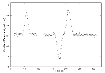
Figure 3: A cross-scan measurement of J0958+3224. First, a scan of the source is made in elevation, during which one beam crosses over the source. A Gaussian function is immediately fitted to this scan and an initial pointing correction is calculated and applied. A scan in azimuth is then performed, where both beams cross over the source. This is fitted using a double Gaussian function, and the final pointing correction is calculated. The initial pointing error is easily noticeable as there is a difference in heights of the beams in the two scans. The one second samples from these scans are shown.

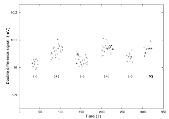
Figure 4: An example of an on-off observation on J1538+4105 (27.6 $\pm$ 1.2 mJy). The first integration is taken when the source is tracked by the secondary beam (marked as (-) on the plot) for 15 seconds (half of the standard integration time of 30 s). Next, three integrations are made, alternating between the primary and secondary beam, followed by a final integration with the source in the secondary beam of the same duration as the first. The last step is an integration at a background position 0.5 deg away in azimuth (marked as ‘bg’).

OCRA-p was used to observe the RT sample between February and October 2007, with additional measurements made during 2008 and early 2009 to complete the sample and check for variability. The pointing positions RT, accurate to better than 10 arcsec, are more than adequate for the 1.2 arcmin OCRA-p beam. Observations of discrete sources are made using two methods. Bright sources (S${}_{30\,\mathrm{GHz}}\mathrel{\mathchoice{\vbox{\offinterlineskip\halign{\hfil$\displaystyle#$\hfil\cr>\cr\simeq\cr}}}{\vbox{\offinterlineskip\halign{\hfil$\textstyle#$\hfil\cr>\cr\sim\cr}}}{\vbox{\offinterlineskip\halign{\hfil$\scriptstyle#$\hfil\cr>\cr\sim\cr}}}{\vbox{\offinterlineskip\halign{\hfil$\scriptscriptstyle#$\hfil\cr>\cr\sim\cr}}}}100$mJy) can be measured using cross-scan observations, where a scan across the source is made first in elevation and then in azimuth (see Figure 3). This method is used both to measure the flux density of target sources (see e.g. Lowe et al., 2007) as well as to determine the required pointing corrections for the telescope (discussed further below). As the sources in the VSA fields are generally too weak for the cross-scan technique, a second method was used whereby the respective two beams, the primary ‘on’ beam and the secondary ‘off’ beam, are pointed at the source alternately with a switching cycle $\sim$50 sec for a period $\sim$5 min, thus measuring the source flux density relative to the background on each side of the source. This method is also used for observing galaxy clusters with OCRA-p (see Lancaster et al., 2007). The switching pattern for this on-off method has evolved during the observations and the final version is shown in Figure 4.

The planetary nebula NGC 7027 was used as our primary flux density calibrator, and was observed at least once per day during the observations of the VSA sources. NGC 7027 is the brightest planetary nebula in the radio sky. Hafez et al. (2008) report a flux density of $5.39\pm 0.04$ Jy at an epoch of 2003.0 at 33 GHz with a secular decrease of $-0.17\pm 0.03$ per cent per year. The flux density at the epoch of 2008.0 is therefore $5.34\pm 0.04$ Jy. We calculate a flux density of $5.47\pm 0.04$ Jy at 30 GHz, using a spectral index of -0.119 (Hafez et al., 2008), and use this to calibrate all of the 30 GHz flux measurements presented in this paper. Zijlstra, van Hoof & Perley (2008) have also obtained accurate data for the flux density of NGC 7027 from which we obtain a value at 30 GHz of $5.37\pm 0.28$ Jy at the epoch of 2008.0, which is consistent with the Hafez et al. (2008) result.

Pointing calibrations are carried out every 30-45 minutes (or every 5-6 on-off measurements). The calibration sources used were J0015+3216 (for field 1L), J0958+3224 (2G), J1521+4336 (3L), J0245+2405 (5E) and J1219+4829 (7E).

4 Data reduction

As the observations are carried out in two different ways – cross-scans across the calibrators and on-offs for the sources – the measured flux densities of the sources are found from two different fitting routines. For the azimuthal cross-scans of the calibration sources, two Gaussian peaks and a quadratic background were fitted, and the average of the two peak heights is used.

The on-off measurements of the VSA sources are fitted by taking a symmetric double difference of the data. In this, the average of an ‘on’ measurement $S_{\mathrm{on}}$ has the average of the second half of the preceding ‘off’ measurement $S_{\mathrm{off,prev}}$ and the first half of the following ‘off’ measurement $S_{\mathrm{off,next}}$ subtracted from it, i.e.

$$S_{\mathrm{dd}}=\frac{1}{N}\sum 0.5\left(S_{\mathrm{on}}-0.5(S_{\mathrm{off,prev}}+S_{\mathrm{off,next}})\right),$$ (1)

where the sum is over all $N$ independent off-on-off sets in the data. As the difference between the measured fluxes is twice the source flux, an extra factor of 0.5 is introduced. The internal error on the measurement is calculated by

$$\sigma_{\mathrm{dd}}=\frac{1}{\sqrt{N}}\sum\sqrt{\left(\frac{\sigma_{S_{\mathrm{on}}}}{2}\right)^{2}+\left(\frac{\sigma_{S_{\mathrm{off,prev}}}}{4}\right)^{2}+\left(\frac{\sigma_{S_{\mathrm{off,next}}}}{4}\right)^{2}}.$$ (2)

Prior to this, any 1 second data points greater than 3 sigma away from the average – representing spikes in the data – are removed.

A noise diode is used for secondary flux density calibration. The ratio of outputs obtained with cross-scans of NGC 7027 and the noise diode are averaged for a 24 hour period; this diode calibration is then applied to the individual measurements.

The change of the telescope gain with elevation was corrected for using a fit to observations of NGC 7027 made over a wide range of elevations. As described by Lowe et al. (2007), atmospheric absorption is corrected for using measurements of the system temperature at the zenith and 60 degrees from zenith made at regular intervals during the observations. A simple ‘flat earth’ model in which the atmosphere is assumed to be a continuous slab with constant thickness and optical depth was used.

A significant number of measurements had to be discarded due to adverse effects of poor weather. Each source was observed multiple times, with individual measurements with large fit errors removed, giving an average of 8.3 observations per source. The final flux density for the source was calculated using the $1/\sigma_{\mathrm{dd}}^{2}$ weighted mean and corresponding standard error on the mean. To ensure the maximum reliability of the results, the observations were reduced separately at the three institutions involved in the OCRA collaboration, with the resulting values compared and discrepancies identified and resolved. The flux densities given in the next section are from one of these reductions; the other reductions give essentially the same values.

The combined uncertainty from these factors is $\sim 8$ per cent. The systematic error due to the error in the flux calibrator, NGC 7027, is negligible at 1 per cent. As such, the final errors on the 30 GHz flux densities are calculated by $\sigma=\sqrt{\sigma_{\mathrm{dd}}^{2}+(0.08S)^{2}}$.

5 Results

Table 1: Sources in the VSA fields. The positions are from the RT 15 GHz observations. Sources marked with a ‘v’ in the note column are variable (see Section 6.1), and those marked with an ‘e’ are extended in FIRST maps (see Section 6.4). Notes on individual sources marked with a * are given in the Appendix. See Section 5 for details.

Name	RA (J2000)	Dec (J2000)	$S_{1.4}$ (mJy)	$S_{4.8}$ (mJy)	$S_{15}$ (mJy)	$S_{30}$ (mJy)	$\alpha_{1.4}^{30}$	Note
J0011+2830	00 11 46.71	28 30 23.1	128.8 $\pm$ 3.9	36 $\pm$ 5	8.8	4.6 $\pm$ 1.1	-1.09${}^{+0.08}_{-0.10}$
J0011+2811	00 11 50.57	28 11 08.4	10.0 $\pm$ 0.5	–	3.6	-2.6 $\pm$ 1.7	$<-0.4$
J0011+2757	00 11 51.72	27 57 18.3	$<$1.5	–	6.0	4.0 $\pm$ 1.0	–
J0012+2821	00 12 01.34	28 21 47.1	8.4 $\pm$ 0.5	–	6.2	-0.7 $\pm$ 0.8	$<-0.5$
J0012+2829	00 12 44.44	28 29 09.5	36.8 $\pm$ 1.2	–	4.4	4.6 $\pm$ 1.5	-0.7 $\pm$ 0.1
J0013+2819	00 13 28.04	28 19 49.5	48.6 $\pm$ 1.5	23 $\pm$ 4	8.4	4.2 $\pm$ 1.7	$<-0.5$
J0013+2834	00 13 32.68	28 34 48.8	39.8 $\pm$ 1.3	32 $\pm$ 5	23.8	14.5 $\pm$ 2.0	-0.33${}^{+0.05}_{-0.06}$	v
J0014+2845	00 14 14.80	28 45 50.9	49.4 $\pm$ 2.1	–	4.6	1.0 $\pm$ 1.6	$<-0.7$
J0014+2821	00 14 16.75	28 21 09.3	263.0 $\pm$ 7.9	56 $\pm$ 6	12.1	1.4 $\pm$ 1.9	$<-1.1$
J0014+2848	00 14 24.78	28 48 44.3	19.7 $\pm$ 0.7	–	2.6	0.9 $\pm$ 3.3	$<-0.2$
(J0014+2852a)	00 14 27.74	28 52 26.8	19.1 $\pm$ 1.0	–	5.5	2.7 $\pm$ 1.3	$<-0.3$	*
(J0014+2852b)	00 14 33.14	28 52 05.1	6.8 $\pm$ 0.5	–	5.4	5.2 $\pm$ 1.0	-0.09${}^{+0.08}_{-0.10}$	*
J0014+2815	00 14 33.84	28 15 05.3	96.0 $\pm$ 2.9	135 $\pm$ 12	45.1	27.6 $\pm$ 2.8	-0.41 $\pm$ 0.04
J0015+2906	00 15 13.97	29 06 13.0	10.6 $\pm$ 0.5	20 $\pm$ 4	5.6	6.5 $\pm$ 1.4	-0.16${}^{+0.08}_{-0.09}$
J0015+2831	00 15 15.45	28 31 53.4	3.7 $\pm$ 1.0	–	3.0	5.4 $\pm$ 2.3	$<1.6$
J0015+2819	00 15 36.64	28 19 22.9	7.1 $\pm$ 0.5	–	2.5	1.2 $\pm$ 1.8	$<0.1$
J0015+2843	00 15 42.48	28 43 39.8	35.7 $\pm$ 1.1	–	7.5	6.9 $\pm$ 1.9	-0.53${}^{+0.09}_{-0.11}$
J0015+2718	00 15 58.02	27 18 53.8	2.1 $\pm$ 1.5	–	3.1	-2.9 $\pm$ 1.6	$<0.4$
J0016+2804	00 16 02.36	28 04 27.4	50.2 $\pm$ 1.6	20 $\pm$ 4	2.7	2.1 $\pm$ 2.7	$<-0.5$
J0017+2733	00 17 04.58	27 33 42.3	11.5 $\pm$ 0.5	–	6.2	2.8 $\pm$ 2.0	$<0.0$
J0017+2750	00 17 23.77	27 50 27.5	302.0 $\pm$ 10.7	88 $\pm$ 8	20.9	11.1 $\pm$ 1.9	-1.08${}^{+0.06}_{-0.07}$
J0017+2835	00 17 32.50	28 35 12.4	82.8 $\pm$ 2.5	35 $\pm$ 5	9.3	4.8 $\pm$ 2.1	$<-0.6$
J0017+2736	00 17 59.94	27 36 16.1	72.8 $\pm$ 2.2	–	4.7	4.4 $\pm$ 1.2	-0.92${}^{+0.09}_{-0.12}$
J0018+2749	00 18 09.49	27 49 24.5	6.2 $\pm$ 0.4	–	10.4	7.0 $\pm$ 1.9	0.0${}^{+0.1}_{-0.1}$
J0018+2843	00 18 11.99	28 43 56.0	17.9 $\pm$ 0.7	–	11.1	4.8 $\pm$ 1.1	-0.43${}^{+0.08}_{-0.10}$	v
J0018+2846	00 18 12.78	28 46 37.6	153.7 $\pm$ 5.3	54 $\pm$ 6	15.0	9.4 $\pm$ 2.0	-0.91${}^{+0.07}_{-0.09}$
J0018+2731	00 18 32.72	27 31 02.9	150.8 $\pm$ 4.5	57 $\pm$ 6	21.2	11.4 $\pm$ 2.0	-0.84${}^{+0.06}_{-0.07}$
J0018+2801	00 18 42.15	28 01 07.9	7.5 $\pm$ 1.0	–	3.7	1.1 $\pm$ 2.7	$<0.2$
J0018+2744	00 18 58.17	27 44 45.5	144.3 $\pm$ 4.3	42 $\pm$ 5	10.0	3.3 $\pm$ 1.3	$<-0.9$
J0019+2817	00 19 08.97	28 17 54.6	24.7 $\pm$ 0.8	–	32.6	26.0 $\pm$ 3.5	0.02${}^{+0.05}_{-0.06}$	v
J0259+2627	02 59 55.32	26 27 29.2	13.8 $\pm$ 0.8	–	9.4	5.5 $\pm$ 1.5	-0.30${}^{+0.10}_{-0.12}$
J0300+2654	03 00 15.58	26 54 52.2	5.3 $\pm$ 0.4	–	5.4	2.7 $\pm$ 1.2	$<0.1$
J0301+2547	03 01 05.43	25 47 16.1	46.3 $\pm$ 1.8	23 $\pm$ 4	14.2	14.6 $\pm$ 2.2	-0.38${}^{+0.06}_{-0.07}$
(J0301+2541)	03 01 37.19	25 41 56.2	300.6 $\pm$ 9.8	92 $\pm$ 9	18.0	10.1 $\pm$ 2.4	-1.11${}^{+0.08}_{-0.10}$	v*
J0301+2521	03 01 38.18	25 21 49.0	134.8 $\pm$ 4.1	44 $\pm$ 5	14.5	8.9 $\pm$ 2.0	-0.89${}^{+0.08}_{-0.09}$
(J0301+2542)	03 01 39.80	25 42 30.1	23.5 $\pm$ 0.8	92 $\pm$ 9	7.2	4.5 $\pm$ 1.5	-0.5 $\pm$ 0.1	*
J0302+2549	03 02 19.94	25 49 49.0	6.7 $\pm$ 0.4	–	7.3	6.9 $\pm$ 1.7	0.01${}^{+0.09}_{-0.11}$
J0302+2607	03 02 42.78	26 07 53.8	77.7 $\pm$ 2.4	34 $\pm$ 5	11.7	6.5 $\pm$ 2.2	$<-0.5$
J0302+2625	03 02 35.72	26 25 53.2	26.6 $\pm$ 0.9	–	3.5	2.7 $\pm$ 1.7	$<-0.4$
J0303+2641	03 03 31.21	26 41 20.9	20.9 $\pm$ 1.0	–	5.0	3.2 $\pm$ 2.1	$<-0.2$
J0303+2645	03 03 34.79	26 45 37.4	365.0 $\pm$ 11.0	102 $\pm$ 10	34.1	15.1 $\pm$ 2.1	-1.04${}^{+0.05}_{-0.06}$
J0303+2700	03 03 58.95	27 00 51.0	3.0 $\pm$ 0.5	–	6.0	3.3 $\pm$ 2.7	$<0.7$
J0303+2531	03 03 59.56	25 31 34.2	153.9 $\pm$ 4.6	122 $\pm$ 11	55.1	45.6 $\pm$ 5.2	-0.40${}^{+0.04}_{-0.05}$	v
J0304+2659	03 04 23.60	26 59 11.0	6.5 $\pm$ 0.7	–	4.2	1.7 $\pm$ 1.2	$<0.1$	*
J0304+2640	03 04 34.02	26 40 03.3	52.1 $\pm$ 1.9	23 $\pm$ 4	6.1	5.4 $\pm$ 1.1	-0.74${}^{+0.07}_{-0.09}$
J0304+2623	03 04 40.82	26 23 10.6	53.1 $\pm$ 2.0	–	4.6	4.1 $\pm$ 1.3	-0.8 $\pm$ 0.1
J0304+2551	03 04 58.58	25 51 49.5	480.8 $\pm$ 14.4	116 $\pm$ 11	28.9	13.4 $\pm$ 1.5	-1.17${}^{+0.04}_{-0.05}$
J0305+2532	03 05 14.96	25 32 16.6	20.3 $\pm$ 0.7	–	5.5	6.0 $\pm$ 1.3	-0.40${}^{+0.07}_{-0.09}$
J0306+2601	03 06 25.43	26 01 21.5	18.7 $\pm$ 0.7	–	7.9	12.6 $\pm$ 2.2	-0.13${}^{+0.07}_{-0.08}$
J0306+2548	03 06 27.66	25 48 22.8	89.2 $\pm$ 2.7	57 $\pm$ 6	18.1	10.7 $\pm$ 1.7	-0.69${}^{+0.06}_{-0.07}$	v
J0306+2627	03 06 32.73	26 27 26.3	95.2 $\pm$ 2.9	25 $\pm$ 4	9.1	1.9 $\pm$ 2.1	$<-0.8$
J0307+2625	03 07 00.33	26 25 48.8	24.4 $\pm$ 0.8	20 $\pm$ 4	20.8	17.6 $\pm$ 4.1	-0.11${}^{+0.08}_{-0.10}$
J0936+3203	09 36 37.43	32 03 31.6	191.2 $\pm$ 5.7	73 $\pm$ 7	22.2	6.1 $\pm$ 1.4	-1.13${}^{+0.08}_{-0.09}$	v
J0936+3118	09 36 53.39	31 18 25.9	21.6 $\pm$ 0.8	–	3.1	-1.4 $\pm$ 2.8	$<-0.3$	e
J0936+3129	09 36 58.25	31 29 29.9	75.9 $\pm$ 8.3	31 $\pm$ 4	5.9	3.0 $\pm$ 2.8	$<-0.5$	e*
J0937+3206	09 37 06.42	32 06 55.4	116.0 $\pm$ 3.5	92 $\pm$ 9	49.3	61.8 $\pm$ 7.9	-0.21 $\pm$ 0.05	e
J0937+3201	09 37 22.63	32 01 03.7	$<$1.5	–	5.3	-0.8 $\pm$ 2.2	–
J0937+3143	09 37 58.41	31 43 41.2	14.6 $\pm$ 0.6	–	6.5	-2.3 $\pm$ 3.2	$<-0.2$

Table 2: continued

Name	RA (J2000)	Dec (J2000)	$S_{1.4}$ (mJy)	$S_{4.8}$ (mJy)	$S_{15}$ (mJy)	$S_{30}$ (mJy)	$\alpha_{1.4}^{30}$	Note
J0938+3118	09 38 17.79	31 18 52.8	24.9 $\pm$ 0.9	22 $\pm$ 4	13.9	6.2 $\pm$ 2.2	$<-0.2$	e
J0939+3134	09 39 48.18	31 34 01.9	34.2 $\pm$ 1.1	–	3.9	5.3 $\pm$ 2.0	$<-0.3$	e
J0939+3154	09 39 50.76	31 54 13.7	96.5 $\pm$ 2.9	30 $\pm$ 4	9.8	6.5 $\pm$ 2.7	$<-0.6$
J0939+3122	09 39 53.86	31 22 43.9	92.4 $\pm$ 3.2	22 $\pm$ 4	8.5	-1.8 $\pm$ 2.5	$<-0.9$	e
J0940+3240	09 40 38.45	32 40 04.8	30.5 $\pm$ 1.0	–	3.4	-3.2 $\pm$ 1.4	$<-1.1$
J0940+3201	09 40 41.85	32 01 31.2	118.5 $\pm$ 3.6	34 $\pm$ 5	12.3	4.6 $\pm$ 1.3	-1.06${}^{+0.09}_{-0.12}$
J0941+3126	09 41 03.32	31 26 20.1	111.1 $\pm$ 3.7	67 $\pm$ 7	20.0	7.2 $\pm$ 3.3	$<-0.6$	e*
J0941+3221	09 41 05.86	32 21 45.3	381.0 $\pm$ 11.4	93 $\pm$ 9	20.2	11.1 $\pm$ 1.8	-1.16${}^{+0.06}_{-0.07}$
J0941+3057	09 41 16.03	30 57 29.2	61.2 $\pm$ 2.3	22 $\pm$ 4	4.4	-1.0 $\pm$ 2.3	$<-0.7$	e
J0941+3146	09 41 46.95	31 46 47.9	3.3 $\pm$ 0.4	–	3.1	0.8 $\pm$ 1.3	$<0.3$
J0941+3154	09 41 47.06	31 54 53.2	288.5 $\pm$ 9.4	99 $\pm$ 9	22.7	12.7 $\pm$ 2.3	-1.02${}^{+0.07}_{-0.08}$	e
J0941+3226	09 41 47.47	32 26 46.1	76.1 $\pm$ 1.2	36 $\pm$ 5	5.4	2.2 $\pm$ 1.8	$<-0.7$	e*
J0942+3239	09 42 00.71	32 39 04.5	16.4 $\pm$ 0.6	–	17.9	8.2 $\pm$ 3.2	$<0.1$
J0942+3206	09 42 08.09	32 06 40.7	189.3 $\pm$ 6.7	62 $\pm$ 7	21.4	10.5 $\pm$ 2.4	-0.94${}^{+0.08}_{-0.10}$	e
J0942+3150	09 42 54.23	31 50 50.6	105.2 $\pm$ 3.9	37 $\pm$ 5	11.8	6.4 $\pm$ 2.6	$<-0.6$	e
J0943+3159	09 43 08.16	31 59 38.0	30.9 $\pm$ 1.0	–	12.5	2.2 $\pm$ 2.4	$<-0.4$	ve
J0943+3132	09 43 44.12	31 32 07.1	33.3 $\pm$ 1.4	–	3.4	-1.3 $\pm$ 2.4	$<-0.5$	e
J0944+3115	09 44 11.60	31 15 21.0	56.2 $\pm$ 2.1	31 $\pm$ 4	24.3	32.1 $\pm$ 3.1	-0.18 $\pm$ 0.04	e
J1227+5240	12 27 17.93	52 40 02.9	26.8 $\pm$ 0.9	–	2.6	2.4 $\pm$ 1.5	$<-0.4$	e
J1227+5313	12 27 52.75	53 13 45.7	12.8 $\pm$ 0.5	–	5.5	4.7 $\pm$ 1.5	-0.3 $\pm$ 0.1
J1228+5308	12 28 19.26	53 08 24.6	6.5 $\pm$ 0.4	–	12.0	2.8 $\pm$ 1.3	$<0.1$
J1230+5230	12 30 08.85	52 30 51.6	74.8 $\pm$ 2.3	24 $\pm$ 4	7.5	-1.0 $\pm$ 1.3	$<-1.0$	e
J1232+5202	12 32 18.49	52 02 19.2	93.0 $\pm$ 2.8	21 $\pm$ 4	9.2	3.9 $\pm$ 2.3	$<-0.7$	e
J1233+5339	12 33 11.08	53 39 56.9	62.6 $\pm$ 1.9	26 $\pm$ 5	24.9	21.3 $\pm$ 2.5	-0.35 $\pm$ 0.05
J1233+5337	12 33 41.38	53 37 27.7	80.8 $\pm$ 2.5	–	6.7	3.6 $\pm$ 0.8	-1.01${}^{+0.08}_{-0.10}$
J1234+5322	12 34 35.89	53 22 35.7	44.0 $\pm$ 1.7	24 $\pm$ 4	5.2	4.4 $\pm$ 1.2	-0.75${}^{+0.09}_{-0.11}$	e
J1235+5317	12 35 00.71	53 17 58.9	5.7 $\pm$ 1.0	–	4.0	4.5 $\pm$ 1.0	-0.1 $\pm$ 0.1	*
J1235+5311	12 35 22.86	53 11 29.0	$<$1.5	–	6.2	5.4 $\pm$ 2.1	–	*
J1235+5210	12 35 29.92	52 10 01.4	166.0 $\pm$ 5.0	41 $\pm$ 5	10.5	3.7 $\pm$ 1.3	$<-1.0$
J1235+5228	12 35 30.53	52 28 27.3	87.5 $\pm$ 2.7	80 $\pm$ 8	47.0	27.3 $\pm$ 2.6	-0.38 $\pm$ 0.04
J1235+5315	12 35 27.86	53 15 01.7	49.2 $\pm$ 2.1	–	6.6	2.6 $\pm$ 1.4	$<-0.6$	e
J1237+5325	12 37 02.19	53 25 25.1	71.5 $\pm$ 2.6	–	9.0	5.1 $\pm$ 2.8	$<-0.5$	e
J1237+5254	12 37 04.16	52 54 22.4	373.5 $\pm$ 14.4	126 $\pm$ 11	35.4	20.1 $\pm$ 2.2	-0.95 $\pm$ 0.05	e
J1237+5303	12 37 25.13	53 03 14.9	51.9 $\pm$ 1.9	24 $\pm$ 4	8.1	3.9 $\pm$ 1.3	-0.8 $\pm$ 0.1	e
(J1238+5249a)	12 38 32.28	52 49 15.8	93.1 $\pm$ 2.8	–	8.3	3.7 $\pm$ 1.1	-1.05${}^{+0.09}_{-0.12}$	*
(J1238+5249b)	12 38 49.78	52 49 34.3	324.9 $\pm$ 9.8	103 $\pm$ 10	34.2	17.5 $\pm$ 2.1	-0.95 $\pm$ 0.05	e*
J1535+4103	15 35 00.62	41 03 13.6	79.1 $\pm$ 2.4	19 $\pm$ 4	5.9	-1.3 $\pm$ 2.2	$<-0.8$	e
(J1535+4143a)	15 35 02.46	41 43 04.8	51.8 $\pm$ 2.2	67 $\pm$ 7	3.5	7.0 $\pm$ 1.2	-0.65${}^{+0.06}_{-0.07}$	e*
(J1535+4143b)	15 35 05.68	41 43 28.2	100.8 $\pm$ 3.7	as above	2.5	6.4 $\pm$ 1.9	-0.90${}^{+0.10}_{-0.13}$	e*
(J1535+4142)	15 35 14.72	41 42 54.0	85.2 $\pm$ 2.6	as above	4.0	5.2 $\pm$ 2.5	$<-0.6$	e*
J1536+4125	15 36 18.07	41 25 38.5	78.5 $\pm$ 2.4	36 $\pm$ 5	8.9	3.9 $\pm$ 2.4	$<-0.6$
J1536+4219	15 36 49.85	42 19 57.5	60.5 $\pm$ 2.2	–	6.3	2.4 $\pm$ 1.5	$<-0.7$	e
J1537+4104	15 37 11.91	41 04 13.0	4.8 $\pm$ 1.1	–	3.3	1.0 $\pm$ 1.5	$<0.4$	e
J1537+4212	15 37 14.86	42 12 53.6	16.4 $\pm$ 0.9	–	9.8	10.2 $\pm$ 2.4	-0.16${}^{+0.09}_{-0.10}$
J1538+4114	15 38 13.93	41 14 06.9	12.4 $\pm$ 0.5	–	7.5	2.1 $\pm$ 2.1	$<-0.1$	e
J1538+4158	15 38 15.57	41 58 28.4	29.9 $\pm$ 1.0	–	5.8	0.8 $\pm$ 2.2	$<-0.4$
J1538+4105	15 38 18.59	41 05 48.4	60.7 $\pm$ 1.9	33 $\pm$ 5	25.4	27.6 $\pm$ 2.5	-0.26 $\pm$ 0.04	e
J1538+4044	15 38 32.10	40 44 55.3	31.3 $\pm$ 1.0	20 $\pm$ 4	3.2	4.4 $\pm$ 1.6	$<-0.4$	e
J1538+4215	15 38 47.13	42 15 27.1	230.5 $\pm$ 8.0	89 $\pm$ 8	25.6	14.9 $\pm$ 2.2	-0.89 $\pm$ 0.06	e
J1538+4225	15 38 55.81	42 25 27.0	57.4 $\pm$ 2.1	44 $\pm$ 5	31.9	27.5 $\pm$ 3.4	-0.24 $\pm$ 0.05	ve
J1539+4120	15 39 10.52	41 20 13.3	4.3 $\pm$ 0.4	–	4.0	6.3 $\pm$ 2.0	0.1${}^{+0.1}_{-0.2}$	e
J1539+4217	15 39 25.63	42 17 28.3	49.0 $\pm$ 1.5	29 $\pm$ 4	31.7	32.1 $\pm$ 3.0	-0.14 $\pm$ 0.04
J1539+4123	15 39 36.78	41 23 34.8	13.8 $\pm$ 0.6	26 $\pm$ 4	31.8	36.2 $\pm$ 3.3	0.31 $\pm$ 0.04
J1539+4148	15 39 38.97	41 48 51.8	3.5 $\pm$ 0.4	–	3.2	0.3 $\pm$ 1.2	$<0.2$	e
J1539+4143	15 39 51.38	41 43 26.4	23.2 $\pm$ 0.8	–	17.3	14.9 $\pm$ 2.7	-0.14${}^{+0.07}_{-0.08}$
J1540+4221	15 40 42.21	42 21 37.3	62.0 $\pm$ 2.5	24 $\pm$ 4	2.5	2.2 $\pm$ 1.1	$<-0.7$	e
J1540+4138	15 40 43.09	41 38 17.4	19.4 $\pm$ 0.7	20 $\pm$ 4	45.6	25.3 $\pm$ 3.3	0.09${}^{+0.05}_{-0.06}$	v
J1541+4114	15 41 01.24	41 14 27.5	48.3 $\pm$ 0.8	53 $\pm$ 6	37.8	15.9 $\pm$ 2.3	-0.36${}^{+0.05}_{-0.06}$	ve*
J1541+4049	15 41 07.17	40 49 17.2	159.7 $\pm$ 5.3	37 $\pm$ 5	10.0	4.4 $\pm$ 1.0	-1.17${}^{+0.08}_{-0.10}$	e
J1541+4122	15 41 47.41	41 22 24.2	7.1 $\pm$ 0.5	–	3.5	1.4 $\pm$ 1.5	$<0.0$	e
J1542+4147	15 42 40.82	41 47 48.3	3.2 $\pm$ 0.4	–	5.2	4.8 $\pm$ 1.3	0.1 $\pm$ 0.1
J1543+4152	15 43 14.37	41 52 24.0	4.2 $\pm$ 0.5	–	5.6	2.0 $\pm$ 1.2	$<0.2$
J1543+4139	15 43 33.09	41 39 32.7	37.9 $\pm$ 1.2	–	5.6	2.0 $\pm$ 1.2	$<0.2$

The source names and J2000.0 positions at 15 GHz are listed in Table 1, along with their flux densities at 15 GHz from the RT observations and at 30 GHz from the OCRA-p observations. We find flux densities for the sources at 1.4 and 4.8 GHz from the NVSS (Condon et al., 1998) and GB6 (Gregory et al., 1996) catalogues by searching for sources within 15 and 60 arcsec, respectively, of the 15 GHz source positions. Flux densities for all but a few sources were found in NVSS, although 50 sources were not present in GB6 principally due to the higher flux density limit of this survey. We calculate the two-point 1.4 to 30 GHz spectral index for the sources, defined such that $S_{\nu}\propto\nu^{\alpha}$.

5.1 Distribution of flux densities

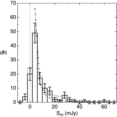
Figure 5: The binned numbers of the source flux densities at 30 GHz, including Poisson errors $(\sqrt{\max(\mathrm{d}N,1)})$ (solid histogram). The simple power law model is also shown (dot-dashed curve). Additionally, a simulated observational histogram (dotted histogram) shows how negative flux densities can occur due to Gaussian errors.

We plot the distribution of 30 GHz flux densities in Figure 5. The negative flux densities for several of the sources listed in Table 1 are consistent with our error estimates. This can be illustrated using a simple model of the set of observed sources. We assume that the sources have been selected randomly from an intrinsic single power law model described by $N(S_{30})=200\;(S_{30}/1\mathrm{mJy})^{-1}$ over the whole survey area, with a sharp minimum flux density limit of $S_{30}=1.7$ mJy, which is the median observational uncertainty. Figure 5 also shows the model and the average histogram from 100 simulated sets of values that would be observed if the model is correct and if the errors are Gaussian errors as listed in Table 1. The histogram of our observations shows reasonable consistency with the model, i.e. the negative flux densities are consistent with random Gaussian errors.

Note that the 1.7 mJy flux limit used here is well below the completeness limit of about 10 mJy (see Section 2.2), so this power law model only provides a rough description of the sample including selection effects; it does not represent the intrinsic source count distribution.

5.2 Source confusion

It is possible that some of the ‘off’ measurements fortuitously fell on previously uncatalogued 30 GHz sources rather than background sky. An upper limit to the level of confusion can be made as follows, by assuming that our sample is complete down to the median observational uncertainty of 1.7 mJy. Since the real completeness limit is about 10 mJy, this should provide a conservative upper limit. Based on the estimate of 31 GHz source counts from Mason et al. (2009), $N(S_{31})\sim 17~{}\mathrm{deg}^{-2}(S_{31}/1\mathrm{mJy})^{-0.8}$, we expect about 0.003 sources/arcmin² above 1.7 mJy. A compatible value is obtained from the much smaller 30 GHz survey by Coble et al. (2007). The OCRA-p beam width is 1.2 arcmin, so the chance of a single ‘off’ measurement landing on an uncatalogued astrophysical object is about 0.003. For any single source, the flux density is estimated as an average from 3–26 (mean: 8.3) individual measurements, each of which uses half the signal from each of two opposite ‘off’ positions (see section 4). The individual measurements for a source are generally made at different position angles, with 3.1 arcmin between ‘on’ and ‘off’ positions. We have 121 sources with 1009 observations of ‘off’ positions. Hence, the expected number of ‘off’ flux densities which are contaminated by uncatalogued objects is about 3.5. The chance that more than one of four contaminating ‘off’ flux densities occur for the same source is $\approx 4.8$ per cent, assuming that clustering effects are negligible. Hence, it would be statistically expected that about four sources each have one contaminated ‘off’ flux density measurement, and no sources have multiple contaminations.

For any of the sources affected by one contaminated ‘off’ flux density measurement, the averaging procedure for the multiple measurements is likely to make the effect of the contamination small, since on average 8.3 measurements are made, and a single ‘off’ flux only contributes half of its value to a given measurement. Hence, on statistical grounds we expect that confusion is negligible for our sample as a whole, though it is likely to have a small effect on a few percent of our sources.

In practice we have direct knowledge of the confusing fields from the RT 15 GHz observations themselves and from the NVSS (Condon et al., 1998) and FIRST (White et al., 1997) catalogues at 1.4 GHz. In a few instances, sources in the RT 15 GHz list are either two parts of the same source or unrelated sources sufficiently close to each other in the sky as to be confused in the present OCRA observations; these are identified by brackets in Table 1. We have examined the NVSS images of all sources and, where available, FIRST images. In the following cases, we conclude that our measured 30 GHz flux densities should be treated with circumspection: J0014+2852a/b, J1535+4142/1535+4143a/b, J0301+2541/42 and J1238+5249a/b. More details on these particular sources are given in the Appendix.

6 Discussion

6.1 Comparison with previous measurements and source variability

Table 3: Comparison of the 15 and 30 GHz flux densities from the RT and OCRA-p (in mJy) from common sources measured with the VLA at 1.4, 4.8, 15.2, 22 and 43 GHz by Bolton et al. (2004); Waldram et al. (2007) and those measured by the source subtractor (Cleary et al., 2005, 2008).

	VLA					RT	OCRA	VSA
Name	$S_{1.4}$	$S_{4.8}$	$S_{15.2}$	$S_{22}$	$S_{43}$	$S_{15}$	$S_{30}$	$S_{33}$	Notes
J0013+2834	32.7	33.1	34.6	36.6	30.5	23.8 $\pm$ 1.2	14.5 $\pm$ 2.0	36.8 $\pm$ 1.8	Variable
J0014+2815	80.4	60.1	45.5	37.7	23.8	45.1 $\pm$ 2.3	27.6 $\pm$ 2.8	34.8 $\pm$ 2.6
J0019+2817	25.9	23.8	17.4	27.0	34.9	32.6 $\pm$ 1.6	26.0 $\pm$ 3.5	23.9 $\pm$ 1.7	Variable (Fig 6)
J0303+2531	–	–	–	–	–	55.1 $\pm$ 2.8	45.6 $\pm$ 5.2	30.0 $\pm$ 2.1
J0937+3206	108.9	53.9	58.4	58.8	41.0	49.3 $\pm$ 2.5	61.8 $\pm$ 7.9	–
J0944+3115	–	–	–	–	–	24.3 $\pm$ 1.2	32.1 $\pm$ 3.1	25.3 $\pm$ 2.6
J1235+5228	–	–	–	–	–	47.0 $\pm$ 2.4	27.3 $\pm$ 2.6	27.9 $\pm$ 1.8
J1539+4123	–	–	–	–	–	31.8 $\pm$ 1.6	36.2 $\pm$ 3.3	33.7 $\pm$ 2.4
J1539+4217	53.3	40.0	34.2	37.0	26.3	31.7 $\pm$ 1.6	32.1 $\pm$ 3.0	34.0 $\pm$ 1.6
J1538+4225	42.0	40.5	41.6	42.2	29.0	31.9 $\pm$ 1.6	27.5 $\pm$ 3.4	41.0 $\pm$ 1.5	Variable
J1540+4138	16.0	30.9	34.2	23.0	9.1	45.6 $\pm$ 2.3	25.3 $\pm$ 3.3	–
J1541+4114	65.0	38.0	30.5	27.5	19.2	37.8 $\pm$ 1.9	15.9 $\pm$ 2.3	32.5 $\pm$ 2.3	Variable

The stronger sources ($>10$mJy at 15 GHz) within the 33 extended VSA fields were observed during the initial VSA campaign at 33 GHz using the VSA source subtractor, with those greater than 20 mJy at 33 GHz used for direct subtraction from the CMB data (Dickinson et al., 2004). A subsample of these was published by Cleary et al. (2005, 2008). Table 3 lists the flux densities measured by the source subtractor for the sources in Cleary et al. (2005, 2008) that also lie within the super-extended array fields, as well as measurements of those sources made at a range of frequencies by Bolton et al. (2004) and Waldram et al. (2007) using the Very Large Array, and compares them to the measurements by the RT and OCRA. A number of the sources show evidence of variability.

Figure 6: The flux density measured for J0019+2817 as a function of time. The source is clearly variable.

We note that OCRA-p is only sensitive to a single linear polarization, which could result in discrepancies between measurements from the VSA, VLA and OCRA for polarized sources; however these are likely to be small since the WMAP sources selected at 22 GHz (see Jackson et al. in preparation) exhibit average linear polarizations of $\sim$3 per cent. The sources observed with the higher resolution interferometers (RT and VLA) may also be slightly resolved. Nevertheless we identify at least four sources (J0013+2834; J1538+4225; J1541+4114; J0019+2817) as likely to be intrinsically variable. One of these sources – J0019+2817 – shows clear variability from OCRA data alone (see Figure 6), although the mean flux density from the measurements agrees well with the source subtractor measurement.

Figure 7: Comparison of the OCRA-p flux densities against those from the VSA source subtractor.

A comparison of flux densities for 42 sources observed both with the VSA source subtractor and OCRA-p is shown in Figure 7. The flux density scales are consistent, however 10 out of the 42 sources show variations greater than $2\sigma$ (combined error), some of which show variations greater than a factor of 2. These are denoted with a ‘v’ in Table 1.

6.2 Source spectra

Figure 8: $\alpha_{1.4}^{4.8}$ vs. $\alpha_{15}^{30}$ for all sources in this sample with a 30 GHz flux density greater than 10 mJy, and known flux densities at all four frequencies. The diagrams in the corners schematically illustrate the spectral behaviour of the sources in each quadrant.

Figure 8 shows the ‘2-colour’ diagram for sources detected at all four frequencies (1.4, 4.8, 15, 30 GHz). We find few sources with peaked spectra (top left quadrant of Figure 8), but a larger number of sources with spectra rising towards high frequencies (right hand quadrants of Figure 8).

Figure 9 displays the distribution of spectral indices $S\propto\nu^{\alpha}$ between 1.4 and 30 GHz for 60 sources above the completeness limit of 7 mJy at 15 GHz (5 out of a total of 65 sources are excluded due to their complex morphology – 0258+2530a/b, 0938+3140 and 1236+5305/6). There is clear evidence of bimodality, with a split around a spectral index of -0.5, dividing the sources into groups of sources with ‘flat’ and ‘steep’ spectra.

The distribution is markedly different from the 1.4 to 30 GHz spectral index distribution presented by Mason et al. (2009). However, their source sample was selected at 1.4 GHz rather than 15 GHz as in this paper. The distribution in Mason et al. (2009) is not bimodal, but has a single peak around $-1.0$, implying that their sample is dominated by the steep spectrum sources. Our sample contains a larger fraction of flat and rising spectrum sources. This is not surprising given the difference of a factor ten in the sample selection frequency.

We return to the issue of spectral indices in different samples in sections 6.3 and 6.4.

6.3 The 1.4-30 GHz spectral index distribution vs flux density

We are seeking to improve our knowledge of the source population at 30 GHz down to mJy flux densities and beyond (by extrapolation). In order to extrapolate one needs to know if there is a dependence of the spectral properties of the population on flux density at 30 GHz. We have therefore used the WMAP 5-year point source catalogue (Wright et al., 2009) to select a complete strong source sample consisting of all sources with a 22 GHz flux above 1 Jy. We have then cross-identified these with the NVSS catalogue and calculated the spectral index distribution between 1.4 and 33 GHz. We chose 22 GHz as the selection frequency to be as close as possible to the 15 GHz selection frequency used in the present paper.

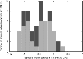
Figure 9: The distribution of spectral indices between 1.4 and 30 GHz ($\alpha_{1.4}^{30}$) for 60 sources in this sample with a 15 GHz flux density greater than 7 mJy. $3\sigma$ detections at 30 GHz are shown in the light grey histogram; the dark grey histogram contains the $3\sigma$ upper limits on the spectral indices.

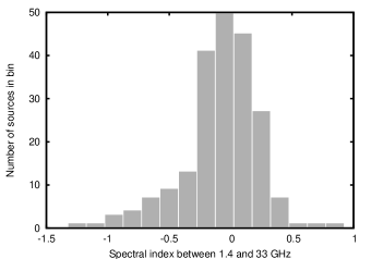
Figure 10: The spectral index distribution of 22 GHz-selected WMAP sources between 1.4 and 33 GHz. The majority of sources have flat spectra ($\alpha>-0.5$).

In this analysis, we exclude sources where there are no obvious NVSS matches, sources known to be extended on scales greater than $\sim 30$ arcmin (WMAP J0322-3711/Fornax A; WMAP J1633+8226/NGC 6251) or confused in WMAP (WMAP J0223+4303/3C66 A and B). Sources are matched to single NVSS sources, except for WMAP J0108+1319/3C33 where four close NVSS sources are combined. In total, 211 sources are used in the analysis. Figure 10 shows the spectral index distribution, which has a single peak centered on zero. All but 16 sources are classified as flat spectrum, i.e. have $\alpha>-0.5$. As expected, this is also very different to the distribution found by Mason et al. (2009), which is dominated by steep spectrum sources.

There is no evidence for a significant population of steep spectrum sources in the WMAP spectral index distribution. This contrasts with the VSA source distribution shown in Figure 9 where there is evidence for both flat and steep spectrum populations. This difference could be ascribed to the selection frequencies (22 GHz cf. 15 GHz), however their closeness suggests that this should not be a major issue. Another consideration is that although we are selecting using the 22 GHz flux densities, in reality the WMAP point source catalogue is obtained using all of the bands (Wright et al., 2009). This should also not be an issue as the sources with 22 GHz flux density greater than 1 Jy are detected by WMAP at high significance. A final possibility, which we think is most likely, is that the dissimilar distributions are due to the difference in the flux densities of the sources in the samples. The population of steep spectrum sources increases as the flux densities decrease.

Such an effect is also seen in Waldram et al. (2009), where they find a significant change in spectral index distribution with flux density amongst their 15 GHz selected sources. We note, however, that there is some overlap in sources between their samples and the one studied here.

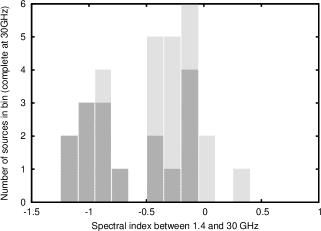
Figure 11: The distribution of spectral indices between 1.4 and 30 GHz ($\alpha_{1.4}^{30}$) for 29 sources in this sample with a 30 GHz flux density greater than 10 mJy. The darker boxes represent sources with flux density between 10 and 20 mJy at 30 GHz; the lighter boxes represent the sources with greater than 20 mJy at 30 GHz. The distribution of the stronger sources closely resembles that of the WMAP sample.

The bimodality of the spectral index distribution remains the same when the sources in this sample are selected at 30 GHz. Figure 11 shows the spectral index distribution of the VSA sources selected to be complete at 30 GHz ($S_{30}>10$ mJy), and Figure 12 shows the spectral indices of WMAP sources selected to be greater than 1 Jy at 33 GHz. Splitting the VSA source sample complete at 30 GHz into high ($>$20 mJy) and low ($<$20 mJy) samples shows that the higher flux density sources have a spectral index distribution closer to the WMAP distribution; the lower flux density sources become increasingly more steep spectrum. A Kolmogorov-Smirnov comparison of the VSA ($S_{30}>10$ mJy) and WMAP distributions shows that the samples are different at the 95 per cent confidence level. The semi-empirical model described by de Zotti et al. (2005) predicts a cross-over between the dominance of flat and steep spectrum sources at about 30 mJy (their Figure 14). Our observations display a sharper cross-over than the models appear to suggest, and at the slightly lower flux density of 20 mJy, but are otherwise consistent with the predictions by de Zotti et al. (2005).

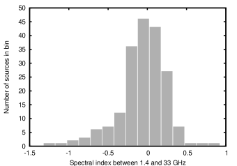
Figure 12: The spectral index distribution between 1.4 and 33 GHz of WMAP sources selected to be stronger than 1 Jansky at 33 GHz. The distribution is essentially the same as for the 22 GHz selected sample, but with slightly fewer sources with spectral indices between 0 and -1.

6.4 Morphological properties

Three of the VSA fields are in the region covered by the FIRST survey (White et al., 1997), and thus 5 arcsec resolution 1.4 GHz maps are available. From a visual inspection of these sources, with contours plotted down to 4 per cent of the peak, we find that 41 of the 68 independent sources (60 per cent) show extended structure; these are marked with an ‘e’ in Table 1. Of these sources, the majority have steep spectra ($\alpha_{1.4}^{30}<-0.5$).

Sixty two sources in the sample of WMAP sources described in the previous section also have FIRST maps available. Again we made a visual inspection of maps with the contours drawn to 4 per cent of the peak flux density. We find that only 21 per cent of these sources are extended, a factor three fewer than in the VSA sample. This difference in the proportion of extended sources between samples containing weak and strong sources reinforces our conclusion, based on spectral indices alone, that the mixture of source types is different in the two samples. It is important to consider if this could arise from differences in selection other than the flux density limit. There are several factors which might bias the content of the samples, often in opposite directions:

• The VSA sources are selected at a lower frequency and therefore there will be a small bias towards more steep spectrum extended sources compared to WMAP.

• The resolutions of the surveys are very different; the RT has a beam of $\sim$30 arcsec at 15 GHz, whilst WMAP has a beam of $0.88^{\circ}$ at 22 GHz. The RT observations will discriminate against sources with structures $\mathrel{\mathchoice{\vbox{\offinterlineskip\halign{\hfil$\displaystyle#$\hfil\cr>\cr\simeq\cr}}}{\vbox{\offinterlineskip\halign{\hfil$\textstyle#$\hfil\cr>\cr\sim\cr}}}{\vbox{\offinterlineskip\halign{\hfil$\scriptstyle#$\hfil\cr>\cr\sim\cr}}}{\vbox{\offinterlineskip\halign{\hfil$\scriptscriptstyle#$\hfil\cr>\cr\sim\cr}}}}$ 30 arcsec i.e. against very extended steep spectrum sources because emission will be resolved out and the sources will drop below the selection limit.

• Some VSA sources are weak and thus in several of the FIRST images extended structure would be more difficult to detect than in the much stronger WMAP sources.

• We do not know the redshift distribution of the VSA sources but being weaker they are likely to be at higher redshift on average than the WMAP sources. This could favour detection of extended structure in the WMAP sources since lower redshift sources will have larger angular sizes and the K-correction will favour higher surface brightness.

On balance we think the known selection effects are slightly biased towards finding more extended WMAP sources. We conclude that the population mix really does depend on flux density.

Is the result unexpected? The magnitude of the effect may be larger than expected but not the sign. There is evidence in the data presented in Orr & Browne (1982) that at 5 GHz the proportion of flat spectrum (and therefore compact) sources decreases with flux density and they show that this is a robust prediction of relativistic beaming models. A clearer observational demonstration of the change of population with flux density can be found in Condon (1984). Condon’s Figures 8 and 9 show that the compact flat spectrum source counts at 5 GHz fall off faster with decreasing flux density than the counts of extended sources. This trend probably does not continue down to $\mu$Jy levels since results on the Hubble Deep Field (e.g. Muxlow et al., 2005) indicate that compact AGN still form about 25 per cent of the population which at these flux density levels is dominated by star-forming galaxies. For studies of the CMB, the exact population mix is not particularly relevant for total intensity observations, however it may well be important for polarized observations since extended AGNs are likely to have higher linear polarizations than their compact counterparts.

In summary, the above results indicate a marked decrease in the proportion of flat-spectrum sources as a function of decreasing flux density. Such a change in population mix may be important for the accurate prediction of polarized foregrounds for CMB experiments.

6.5 Comparison of estimates of source surface densities at 30 GHz

There are 31 sources in the five VSA fields detected above 10 mJy at 30 GHz. These effectively comprise a complete sample as the sources were selected from a deeper survey at the nearby frequency of 15 GHz. The surface density of sources is thus $2\pm 0.4$ sources per square degree (using the Poissonian error), which can be compared with the extrapolated value of $2.65\pm 0.1$ in Mason et al. (2009). Coble et al. (2007) also give an estimate of the surface density of 30 GHz sources in the field, which gives $2.2^{+2.5}_{-1.2}$ sources per square degree; they also point out that the density of sources in clusters of galaxies is significantly higher.

7 Conclusion

In order to aid the subtraction of individual sources from the VSA fields observed at $\sim$30 GHz, and to obtain a statistical estimate of the surface density of sources at 30 GHz, we have observed a sample of 121 sources using the OCRA-p receiver on the Toruń 32 m telescope; the sample was selected at 15 GHz with the RT. At 30 GHz, we detected 57 sources above a limiting flux density of $\sim 5$ mJy. This is the deepest follow-up of any complete sample of sources detected at 15 GHz by the RT.

At a flux density of 10 mJy, which is our estimated completeness limit, we derive a surface density of sources at 30 GHz of $2.0~{}\pm~{}0.4$ per square degree. This is consistent with the value obtained by Mason et al. (2009), who observed a much larger sample of sources down to mJy levels but selected at a much lower frequency (1.4 GHz). The potential danger of using low frequency selected samples is that there may exist a significant population of sources with steeply rising spectra towards high frequencies that are not present in the low frequency surveys. As the two surface density estimates are consistent, this indicates that such a population is not obviously present at the 10 mJy level.

We have compared our flux density measurements with those from the VSA source subtractor and VLA measurements. These comparisons give confidence in our flux scale but reveal that a significant fraction of sources are variable on a timescale of a few years, some at the level of a factor of 2. This shows the importance of taking contemporaneous measurements of discrete sources in conjunction with measurements of the CMB.

We have also investigated the dependence of the spectral index distribution on flux density by comparing our measured spectral index distribution with that for much stronger sources (above 1 Jy) selected from the WMAP 22 GHz catalogue. We conclude that the proportion of steep spectrum sources increases with decreasing flux density. This is qualitatively consistent with models of source populations, for example de Zotti et al. (2005).

Appendix: Notes on individual sources

• J0014+2852a/b – probably two components of a single source separated by 75 arcsec and our listed 30 GHz flux densities are blends of both components. Not used in the spectral analysis.

• J0301+2541/42 – are separated by $\leq$1 arcmin and are probably part of the same source. Their flux densities are blended in our 30 GHz measurements. Not used in the spectral analysis.

• J0304+2659 – 15 GHz position is $\sim 15$ arcsec south of NVSS peak.

• J0936+3129 – Double source in FIRST map, RT source coincident with western component.

• J0941+3126 – the FIRST and NVSS maps show that this source has two extended components. This source is not used in the spectral analysis.

• J0941+3226 – NVSS and FIRST show 15 GHz component is at the southern end of an extended source.

• J1235+5317 – 15 GHz position is $\sim 55$ arcsec south-east of NVSS peak.

• J1235+5311 – no 1.4 GHz sources are detected in the NVSS or FIRST maps at the RT position but weak extended components straddle this position in the NVSS map.

• J1238+5249a/b – are separated by approximately 2.5 arcmin east-west and thus for half the on-off observations of each source the other lies within the reference beam. The correction, however, is very small.

• J1535+4142 and J1535+4143a/b – lie within 3 arcmin of each other. Examination of the FIRST map of the region suggests that they may be physically related. Our 30-GHz flux density measurements are confused. Not used in the spectral analysis.

• J1541+4114 – NVSS and FIRST maps show that 15 GHz component is probably the central component of an asymmetric triple source.

References

- Bolton et al. (2004) Bolton, R. C. et al., 2004, MNRAS, 354, 485
- Browne et al. (2000) Browne I. W. A., Mao S., Wilkinson P. N., Kus A. J., Marecki A., Birkinshaw M., 2000, in Butcher H. R., ed., Proc. SPIE Vol. 4015, Radio Telescopes SPIE, New York, p. 299
- Cleary et al. (2005) Cleary, K. A. et al., 2005, MNRAS, 360, 340
- Cleary et al. (2008) Cleary, K. A. et al., 2008, MNRAS, 386, 1759 (Erratum)
- Coble et al. (2007) Coble, K. et al., 2007, AJ, 134, 897
- Condon (1984) Condon, J. J., 1984, ApJ, 287, 461
- Condon et al. (1998) Condon, J. J., Cotton, W. D., Greisen, E. W., Yin, Q. F., Perley, R. A., Taylor, G. B., Broderick, J. J., 1998, AJ, 115, 1693
- Dickinson et al. (2004) Dickinson, C. et al., 2004, MNRAS, 353, 732
- Friedman et al. (2009) Friedman R. B., et al., 2009, ApJ, 700, L187
- Grainge et al. (2003) Grainge K. et al., 2003, MNRAS, 341, L23
- Gregory et al. (1996) Gregory P. C., Scott W. K., Douglas K., Condon J. J., 1996, ApJS, 103, 427
- Hafez et al. (2008) Hafez, Y.A. et al., 2008, MNRAS, 388, 1775
- Hinshaw et al. (2003) Hinshaw G. et al., 2003, ApJS, 148, 135
- Hinshaw et al. (2009) Hinshaw G. et al., 2009, ApJS, 180, 225
- Jones et al. (2006) Jones W. C. et al., 2006, ApJ, 647, 823
- Komatsu et al. (2009) Komatsu E. et al., 2009, ApJS, 180, 330
- Lancaster et al. (2007) Lancaster K. et al., 2007, MNRAS, 378, 673
- Lowe et al. (2007) Lowe S. R., Gawroński M. P., Wilkinson P. N., Kus A. J., Browne I. W. A., Pazderski E., Feiler R., Kettle D., 2007, A&A, 474, 1093
- Mason et al. (2003) Mason B. S. et al., 2003, ApJ, 591, 540
- Mason et al. (2009) Mason B.S., Weintraub L.C., Sievers J.L., Bond J.R., Myers S.T., Pearson T.J., Readhead A.C.S., Shepherd M.C., 2009, preprint (arXiv:0901.4330)
- Muxlow et al. (2005) Muxlow, T. W. B. et al., 2005, MNRAS, 358, 1159
- Orr & Browne (1982) Orr, M. J. L. and Browne, I. W. A., 1982, MNRAS, 200, 1067
- Pazderska et al. (2009) Pazderska B. M. et al., 2009, A&A, 498, 463
- Peel, Battye & Kay (2009) Peel M., Battye R., Kay S., 2009, MNRAS, 397, 2189
- Readhead et al. (2004) Readhead A.C.S. et al., 2004, ApJ, 609, 498
- Reichardt et al. (2009) Reichardt B.S. et al., 2009, ApJ, 694, 1200
- Sharp et al. (2009) Sharp M.K. et al., 2009, preprint (arXiv:0901.4342)
- Shaw et al. (2009) Shaw L., Zahn O., Holder G., Dore O., 2009, ApJ, 702, 368
- Sievers et al. (2009) Sievers J.L. et al., 2009, preprint (arXiv:0901.4540)
- Smoot et al. (1992) Smoot G. F. et al., 1992, ApJL, 396, L1
- Toffolatti et al. (1998) Toffolatti L., Argueso Gomez F., de Zotti G., Mazzei P., Franceschini A., Danese L., Burigana C., 1998, MNRAS, 297, 117
- Toffolatti et al. (2005) Toffolatti L., Negrello M., Gonz lez-Nuevo J., de Zotti G., Silva L., Granato G. L., Argüeso F., 2005, A&A, 438, 475
- Waldram et al. (2003) Waldram E. M., Pooley G. G., Grainge K. J. B., Jones M. E., Saunders R. D. E., Scott P. F., Taylor A. C., 2003, MNRAS, 342, 915
- Waldram et al. (2007) Waldram E. M., Bolton R. C., Pooley G. G., Riley J. M., 2007, MNRAS, 379, 1442
- Waldram et al. (2009) Waldram E. M., Pooley G. G., Davies M. L., Grainge K. J. B. and Scott P. F., 2009, preprint (arXiv:0908.0066)
- Wright et al. (2009) Wright E. L. et al., 2009, ApJS, 180, 283
- White et al. (1997) White R.L., Becker R.H., Helfand D.J., Gregg M.D., 1997, ApJ, 475, 479
- Zijlstra, van Hoof & Perley (2008) Zijlstra A. A., van Hoof P. A., M., Perley R. A., 2008, ApJ, 681, 1296
- de Zotti et al. (2005) de Zotti, G. and Ricci, R. and Mesa, D. and Silva, L. and Mazzotta, P. and Toffolatti, L. and González-Nuevo, J., 2005, A&A, 431, 893