Abstract

A general approach describing quantum decision procedures is developed. The approach can be applied to quantum information processing, quantum computing, creation of artificial quantum intelligence, as well as to analyzing decision processes of human decision makers. Our basic point is to consider an active quantum system possessing its own strategic state. Processing information by such a system is analogous to the cognitive processes associated to decision making by humans. The algebra of probability operators, associated with the possible options available to the decision maker, plays the role of the algebra of observables in quantum theory of measurements. A scheme is advanced for a practical realization of decision procedures by thinking quantum systems. Such thinking quantum systems can be realized by using spin lattices, systems of magnetic molecules, cold atoms trapped in optical lattices, ensembles of quantum dots, or multilevel atomic systems interacting with electromagnetic field.

Key words: quantum information processing, quantum computing, quantum decision procedures, artificial quantum intelligence

PACS numbers: 02.50.Le, 03.65.Ta, 03.67.Hk

1 Introduction

The study of different processes realized by and with quantum systems is of great importance for many problems, from the well established quantum measurements [1] to the currently developing fields of quantum information processing and quantum computation [2-7]. In all these cases, one considers procedures accomplished by an external observer over a passive quantum system. The principal question we address in the present paper is whether a quantum system could be active, and take decisions in a way similar to decision making performed by human beings. That is, could a quantum system think, as humans do? Answering this question is vital for understanding whether a quantum artificial intelligence could be created.

It is necessary to stress that the description of human thinking processes we have in mind does not refer to the physiological mechanisms occurring in the brain, but rather concerns the general mathematical scheme that may be developed for formalizing such processes. Anticipating on our main theme, if the human thinking process could be formalized by a quantum mechanics based approach, it would then be straightforward to attempt realizing a scheme of such a process by using a suitable quantum system.

In order to answer the above question, it is necessary, first of all, to assess whether it is possible to describe the process of human thinking in terms of the quantum mechanical language. Actually, Bohr [8] conjectured that the processes involved in human thinking are similar to quantum operations, and hence could be described by the language of quantum theory. This is in contrast with the standard way of characterizing the process of human thinking, which is well formalized by classical decision theory, whose mathematical foundation is due to von Neumann and Morgenstern [9]. This classical approach explains the process of human decision making as being based on the evaluation of expected utility. Despite its normative appeal, the classical expected utility theory is confronted with a number of paradoxes, when compared with decision making of real human beings [10].

If we were to follow the Bohr’s idea [8] that the human thinking processes can be described by means of quantum theory, we should stress that this possibility does not require the assumption that humans are some quantum systems. Instead, it holds that the process of human thinking can be mathematically formalized in the language of quantum theory, similarly to the process of quantum measurement [11]. To make our point clear, consider the analogous situation presented by the theory of differential equations, which was initially developed for describing the motion of planets. The theory of differential equations is now employed everywhere, being just an efficient mathematical tool. In the same way, we explore here the possibility that quantum theory may provide a convenient framework for the mathematical description of thinking processes.

The aim of the present paper is twofold. First, we give a general mathematical scheme of how decision making can be described in the language of quantum theory. The scheme is general in the sense that it can be equally applied to human decision makers and to active quantum systems imitating the process of taking decisions. Second, we suggest the principal architecture for such thinking quantum systems and discuss how it could be realized by real physical systems, such as ensembles of spins, atoms, molecules, or quantum dots.

2 Mathematical Scheme

To be precise, we first formulate the mathematical scheme characterizing the process of decision making in the language of quantum theory.

Definition 1. Action ring

The process of taking decisions implies that one is deliberating between several admissible actions with different outcomes, in order to decide which of the intended actions to choose. Therefore, the first element arising in decision theory is an intended action $A$. The set of these admissible intended actions can be enumerated with an index $i=1,2,...,N$, where the total number $N$ of actions can be finite or infinite. The whole family of all these actions forms the action set

$${\cal A}\equiv\{A_{i}:\;i=1,2,\ldots,N\}\;.$$ (1)

The elements of this set are assumed to be endowed with two binary operations, addition and multiplication, so that, if $A$ and $B$ pertain to ${\cal A}$, then $AB$ and $A+B$ also pertain to ${\cal A}$. The addition is associative, such that $A+(B+C)=(A+B)+C$, and reversible, in the sense that $A+B=C$ implies $A=C-B$. The multiplication is distributive, $A(B+C)=AB+BC$, and idempotent, $AA=A$. The latter means that an intended action, being thought of twice, is the same action. The multiplication is not necessarily commutative, so that, generally, $AB$ is not the same as $BA$. Among the elements of the action set (1), there is an identical action $1$, for which $A1=1A=A$. And there exists an impossible action $0$, for which $A0=0A=0$. Two actions are called disjoint, when there joint action is impossible, giving $AB=BA=0$. The action set (1), with the described structure, is termed the action ring.

Definition 2. Action modes

An action is simple, when it cannot be decomposed into the sum of other actions. An action is composite, when it can be represented as a sum of several other actions. If an action is represented as a sum

$$A_{i}=\bigcup_{\mu=1}^{M_{i}}A_{i\mu}\;,$$ (2)

whose terms are mutually incompatible, then these terms are named the action modes. The modes correspond to different possible ways of realizing an action.

Definition 3. Elementary prospects

Generally, decision taking is not necessarily associated with a choice of just one action among several simple given actions, but it involves a choice between several complex actions. The simplest such complex action is defined as follows. Let the multi-index $n=\{\nu_{1},\nu_{2},...,\nu_{N}\}$ be a set of indices enumerating several chosen modes, under the condition that each action is represented by one of its modes. The elementary prospect is the conjunction

$$e_{n}\equiv\bigcap_{i=1}^{N}A_{i\nu_{i}}\;,$$ (3)

of the chosen modes, one for each of the actions from the action ring (1). The total set of all elementary prospects will be denoted as $\{e_{n}\}$.

Definition 4. Composite prospects

A prospect is composite, when it cannot be represented as an elementary prospect (3). Generally, a composite prospect is a conjunction

$$\pi_{j}=\bigcap_{n}A_{j_{n}}$$ (4)

of several composite actions of form (2), where each of the factors $A_{j_{n}}$ pertains to the action ring (1).

Definition 5. Prospect lattice

All possible prospects, among which one needs to make a choice, form a set

$${\cal L}=\{\pi_{j}:\;j=1,2,\ldots,N_{L}\}\;.$$ (5)

The set is assumed to be equipped with the binary relations $>,<,=,\geq,\leq$, so that each two prospects $\pi_{i}$ and $\pi_{j}$ in $\cal L$ are related as either $\pi_{i}>\pi_{j}$, or $\pi_{i}=\pi_{j}$, or $\pi_{i}\geq\pi_{j}$, or $\pi_{i}<\pi_{j}$, or $\pi_{i}\leq\pi_{j}$. For a while, it is sufficient to assume that such an ordering exists. Then, the ordered set (5) is called a lattice. The explicit ordering procedure associated with decision making will be given below.

Definition 6. Mode space

To each action mode $A_{i\mu}$, there corresponds the mode state $|A_{i\mu}\rangle$, which is a complex function ${\cal A}\rightarrow{\cal C}$, and its Hermitian conjugate $\langle A_{i\mu}|$. Here we employ the Dirac notation [12]. We assume that a scalar product is defined, such that the mode states, pertaining to the same action, are orthonormalized:

$$\langle A_{i\mu}|A_{i\nu}\rangle=\delta_{\mu\nu}\;.$$ (6)

The mode space is the closed linear envelope

$${\cal M}_{i}\equiv{\rm Span}\{|A_{i\mu}\rangle:\;\mu=1,2,\ldots,M_{i}\}\;,$$ (7)

spanning all mode states. By this definition, the mode space, corresponding to an $i$-action $A_{i}$, is a Hilbert space of dimensionality $M_{i}$.

Definition 7. Mind space

To each elementary prospect $e_{n}$ there corresponds the basic state $|e_{n}\rangle$, which is a complex function ${\cal A}^{N}\rightarrow{\cal C}$, and its Hermitian conjugate $\langle e_{n}|$. The structure of a basic state is

$$|e_{n}\rangle\equiv|A_{1\nu_{1}}A_{2\nu_{2}}\ldots A_{N\nu_{N}}\rangle=\bigotimes_{i=1}^{N}|A_{i\nu_{i}}\rangle\;.$$ (8)

The scalar product is assumed to be defined, such that the basic states are orthonormalized:

$$\langle e_{m}|e_{n}\rangle=\prod_{i=1}^{N}\delta_{\mu_{i}\nu_{i}}\equiv\delta_{mn}\;.$$ (9)

The mind space is the closed linear envelope

$${\cal M}\equiv{\rm Span}\{|e_{n}\rangle\}=\bigotimes_{i=1}^{N}{\cal M}_{i}\;,$$ (10)

spanning all basic states (8). Hence, the mind space is a Hilbert space of dimensionality

$${\rm dim}{\cal M}=\prod_{i=1}^{N}M_{i}\;.$$

The vectors of the mind space represent all possible actions and prospects considered by a decision maker.

Definition 8. Prospect states

To each prospect $\pi_{j}$ there corresponds a state $|\pi_{j}\rangle\in{\cal M}$ that is a member of the mind space (10). Hence, the prospect state can be represented as an expansion over the basic states

$$|\pi_{j}\rangle=\sum_{n}\;a_{jn}|e_{n}\rangle\;.$$ (11)

The prospect states are not required to be mutually orthogonal and normalized to one, so that the scalar product

$$\langle\pi_{i}|\pi_{j}\rangle=\sum_{n}\;a_{in}^{*}a_{jn}$$

is not necessarily a Kronecker delta.

Definition 9. Strategic state

Among the states of the mind space, there exists a special fixed state $|s\rangle\in{\cal M}$, playing the role of a reference state, which is termed the strategic state. This is the state characterizing the specific decision maker. Being in the mind space (10), this state can be represented as the decomposition

$$|s\rangle=\sum_{n}c_{n}|e_{n}\rangle\;.$$ (12)

Being a unique state, characterizing each decision maker like its fingerprints, it can be normalized to one:

$$\langle s|s\rangle=1\;.$$ (13)

From Eqs. (12) and (13), it follows that

$$\sum_{n}|c_{n}|^{2}=1.$$

The existence of the strategic state, uniquely defining each particular decision maker, is the principal point distinguishing the active thinking quantum system from a passive quantum system subject to measurements from an external observer. For a passive quantum system, predictions of the outcome of measurements are performed by summing (averaging) over all possible statistically equivalent states, which can be referred to as a kind of “annealed” situation. In contrast, decisions and observations associated with a thinking quantum system occur in the presence of this unique strategic space, which can be thought of as a kind of fixed “quenched” state. As a consequence, the outcomes of the applications of the quantum mechanical formalism will thus be different for thinking versus passive quantum systems.

Definition 10. Prospect operators

Each prospect state $|\pi_{j}\rangle$, together with its Hermitian conjugate $\langle\pi_{j}|$, defines the prospect operator

$$\hat{P}(\pi_{j})\equiv|\pi_{j}\rangle\langle\pi_{j}|\;.$$ (14)

By this definition, the prospect operator is self-adjoint. The family of all prospect operators forms the involutive bijective algebra that is analogous to the algebra of local observables in quantum theory. Since the prospect states, in general, are neither mutually orthogonal nor normalized, the squared operator

$$\hat{P}^{2}(\pi_{j})=\langle\pi_{j}|\pi_{j}\rangle\hat{P}(\pi_{j})$$

contains the scalar product

$$\langle\pi_{j}|\pi_{j}\rangle=\sum_{n}|a_{nj}|^{2}\;,$$

which does not equal to one. This tells us that the prospect operators, generally, are not idempotent, thus, they are not projection operators. It is only when the prospect is elementary that the related prospect operator

$$\hat{P}(e_{n})=|e_{n}\rangle\langle e_{n}|$$

becomes idempotent and is a projection operator. But, in general, this is not so.

Definition 11. Prospect probabilities

In quantum theory, the averages over the system state, for the operators from the algebra of local observables, define the observable quantities. In the same way, the averages, over the strategic state, for the prospect operators define the observable quantities, the prospect probabilities

$$p(\pi_{j})\equiv\langle s|\hat{P}(\pi_{j})|s\rangle\;.$$ (15)

These are assumed to be normalized to one:

$$\sum_{j=1}^{N_{L}}\;p(\pi_{j})=1\;,$$ (16)

where the summation is over all prospects from the prospect lattice (5). By their definition, quantities (15) are non-negative, since Eq. (15) reduces to the modulus of the transition amplitude squared

$$p(\pi_{j})=|\langle\pi_{j}|s\rangle|^{2}\;.$$

Being normalized as in Eq. (16), the set $\{p(\pi_{j})\}$ composes the scalar probability measure.

Definition 12. Utility factor

The diagonal form

$$p_{0}(\pi_{j})\equiv\sum_{n}\;\langle s|\hat{P}(e_{n})\hat{P}(\pi_{j})\hat{P}(e_{n})|s\rangle$$ (17)

plays the role of the expected utility in classical decision making, justifying its name as the utility factor. In order to be generally defined and to be independent of the chosen units of measurement, the factor (17) can be normalized as

$$\sum_{j=1}^{N_{L}}\;p_{0}(\pi_{j})=1\;.$$ (18)

The fact that factor (17) is really equivalent to the classical expected utility follows from noticing that

$$\hat{P}(e_{n})|s\rangle=c_{n}|s\rangle\;,$$

hence Eq. (17) acquires the form

$$p_{0}(\pi_{j})=\sum_{n}|c_{n}|^{2}\langle e_{n}|\hat{P}(\pi_{j})|e_{n}\rangle\;,$$

where $<e_{n}|\hat{P}(\pi_{j})|e_{n}>$ plays the role of a utility function, weighted with the probability $|c_{n}|^{2}$.

Definition 13. Attraction factor

The nondiagonal term

$$q(\pi_{j})\equiv\sum_{m\neq n}\;\langle s|\hat{P}(e_{m})\hat{P}(\pi_{j})\hat{P}(e_{n})|s\rangle$$ (19)

arises as a consequence of the quantum interference effect. Its appearance is typical of quantum mechanics. Such nondiagonal terms do not occur in classical decision theory. This term can be called the interference factor. Interpreting its meaning in decision making, we can associate its appearance as resulting from the system deliberation between several alternatives, when deciding which of the latter is more attractive. Thence, the name “attraction factor.” Using expansion (12) in Eq. (19) yields

$$q(\pi_{j})\equiv\sum_{m\neq n}c_{m}^{*}c_{n}\langle e_{m}|\hat{P}(\pi_{j})|e_{n}\rangle\;,$$

which shows that the interference occurs between different elementary prospects in the process of considering a composite prospect $\pi_{j}$. It is worth stressing that the interference factor is nonzero only when the prospect $\pi_{j}$ is composite. If it were elementary, say $\pi_{j}=e_{k}$ then, since

$$\hat{P}(e_{k})|e_{n}\rangle=\delta_{nk}|e_{n}\rangle\;,$$

we would have

$$q(e_{k})=\sum_{m\neq n}c_{m}^{*}c_{n}\delta_{mn}\delta_{nk}=0\;,$$

and no interference would arise.

Definition 14. Prospect ordering

In defining the prospect lattice (5), we have assumed that the prospects could be ordered. Now, after introducing the scalar probability measure, we are in a position to give an explicit prescription for the prospect ordering. We say that the prospect $\pi_{1}$ is preferable to $\pi_{2}$ if and only if

$$p(\pi_{1})>p(\pi_{2})\qquad(\pi_{1}>\pi_{2})\;.$$ (20)

Two prospects are called indifferent if and only if

$$p(\pi_{1})=p(\pi_{2})\qquad(\pi_{1}=\pi_{2})\;.$$ (21)

And the prospect $\pi_{1}$ is preferable or indifferent to $\pi_{2}$ if and only if

$$p(\pi_{1})\geq p(\pi_{2})\qquad(\pi_{1}\geq\pi_{2})\;.$$ (22)

These binary relations provide us with an explicit prospect ordering making the prospect set (5) a lattice.

Definition 15. Optimal prospect

Since all prospects in the lattice are ordered, it is straightforward to find among them that one enjoying the largest probability. This defines the optimal prospect $\pi_{*}$ for which

$$p(\pi_{*})\equiv\sup_{j}p(\pi_{j})\;.$$ (23)

Finding the optimal prospect is the final goal of the decision-making process. Since the prospect probabilities are non-negative, it is possible to find the minimal prospect in the lattice (5) with the smallest probability. And the largest probability defines the optimal prospect $\pi_{*}$. Therefore the prospect set (5) is a complete lattice.

From the above definitions, we get the following theorem.

Theorem. The prospect probability (15) has the form

$$p(\pi_{j})=p_{0}(\pi_{j})+q(\pi_{j})\;,$$ (24)

in which the attraction factor (19) satisfies the alternation property

$$\sum_{j=1}^{N_{L}}\;q(\pi_{j})=0\;,$$ (25)

where the summation is over the whole lattice $\cal L$.

Proof. Substituting into definition (15) expansion (12) and invoking Eqs. (17) and (19) gives expression (24). Employing the normalization conditions (16) and (18) results in the alternation property (25).

The above definitions and the theorem constitute the basic mathematical structure of the Quantum Decision Theory (QDT), which can be applied to different decision makers, whether these are human beings or quantum systems.

3 Physical Scheme

3.1. General scheme of a thinking quantum machine

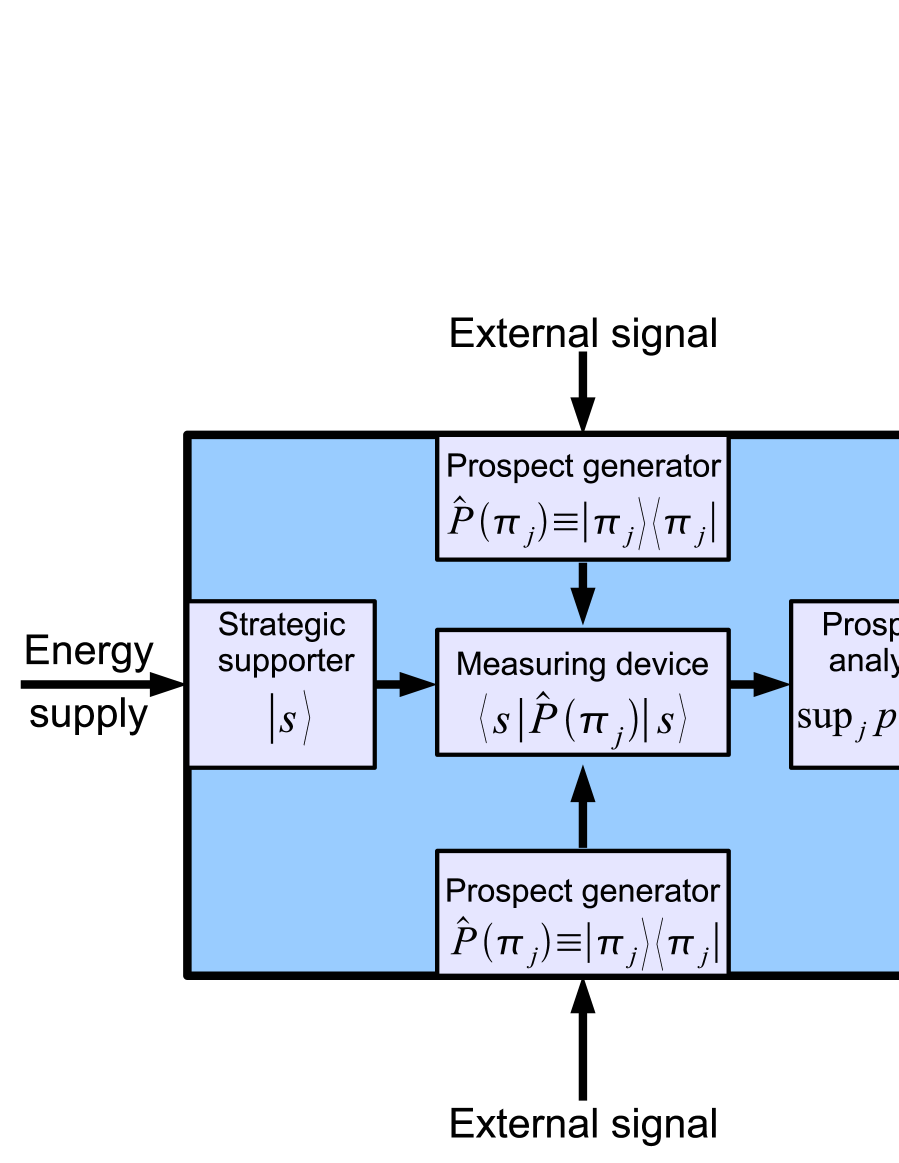
Figure 1: Principal scheme of a thinking quantum system, imitating the process of decision making.

The basic elements of a thinking quantum machine are as follows. As is evident, no decision maker can be in equilibrium and be a closed system. Therefore, there should be an external energy supply supporting the strategic state characterizing the particular decision maker. The prospect states are also imposed from outside, representing the information loaded into the system, about which a decision is to be taken. Measuring the averages of the prospect operators is equivalent to measuring the averages of observable quantities. In the present case, the prospect states are scattered over the strategic state. The measurement procedure results in the scattering cross-sections that are proportional to the scattering amplitudes squared. The latter define the prospect probabilities. The prospect analyzer selects the largest probability, and in so doing chooses the optimal prospect. The state corresponding to the optimal prospect is the system output. This summarizes how the system processes information, imitating the procedure of human decision making, as shown in Fig. 1.

3.2. Physical embodiment of thinking quantum machines

Let us now suggest different physical quantum systems that could realize the process of decision making based on the mathematical theory of Sec. 2 and on the general scheme of the previous subsection illustrated by Fig. 1. Several physical systems can be used for this purpose. The main requirement is that the system would be composed of several parts, enumerated with an index $i=1,2,...,N$, and that, in each $i$-part, mode states $|A_{i\mu}\rangle$ could be generated. Such systems can be realized with real-space lattices or nanostructures. Below, we discuss several possible physical realizations.

(i) Real-space lattice of spins

Such a very convenient system is the real-space lattice of spins. Then the mode state $|A_{i\mu}\rangle$ is the spin state in the $i$-lattice site, with the $\mu$-spin projection. The basic states $|e_{n}\rangle$ are the lattice spin states forming the basis for the given lattice. The prospect states $|\pi_{j}\rangle$ are the states produced by external fields that play the role of information provided to the system. The strategic state $|s\rangle$ is a chosen state supported by means of additional energy supply. Different nontrivial many-body spin states can be created by applying, for instance, staggered magnetic fields to a spin lattice [13]. In some cases [14], the staggered magnetization arises in spin systems by its own. The spins in a lattice can be of different physical nature and of different type. Promising candidates could be magnetic molecules having high spins, hence providing a number of modes in each lattice site (see details in review articles [15-18]). The manipulation with magnetic molecules can be realized by swiping magnetic fields. An ultrafast manipulation with lattice spins can be done by connecting the sample to a resonator, which makes it possible to create various regimes of spin motion [17-25]. Magnetic clusters of high spins [26,27] can be used as well. Their spins can also be manipulated by external magnetic fields, achieving a fast regulation in the presence of a resonator [17,18,23-25].

(ii) Optical lattices of cold Bose-condensed atoms

Optical lattices of cold Bose-condensed atoms could be another physical system allowing one to create various atomic states [28-33]. When each lattice site contains many condensed bosons, it is possible [34-36] to realize a resonant generation of coherent topological modes in each of the lattice sites. Then the mode state $|A_{i\mu}\rangle$ is a $\mu$-type coherent mode in the lattice $i$-site. The manipulation of the modes can be accomplished by means of a magnetic field modulation for atoms trapped in the lattice sites [34-36] or by modulating the atomic scattering length by means of Feshbach resonance techniques [37]. The overall setup is similar to that of the spin systems.

(iii) Bosons or fermions in double-well optical lattices

In the case of double-well optical lattices [38-42], one can use bosons as well as fermions by creating different insulating states related to atoms shifted into one or another well of a double well [43-45], with the index $\mu$ marking the left or right side of a double well. Then the mode state $|A_{i\mu}\rangle$ corresponds to the left or right position of an atom in a double well located at the lattice $i$-site. By varying the parameters of a double well, different atomic states can be created [43-46].

(iv) Multilevel radiating atoms or molecules inside a solid-state matrix

Multilevel radiating atoms or molecules inside a solid-state matrix can also be used, provided it is feasible to transfer each of the atoms into the required energy states by applying external laser beams. The state $|A_{i\mu}\rangle$ is then the state of an $i$-atom on the $\mu$-level. Atomic interactions through the common radiation field would result in highly correlated coherent states of the whole system [47,48]. Multilevel atoms seem to be a convenient tool for realizing quantum computation and quantum information processing [49,50].

(v) Nanostructures

Nanostructures, such as quantum dots, quantum wells, and quantum wires, possessing discrete energy levels, are known [51-54] to have properties similar to multilevel atoms, justifying their name “artificial atoms”. Therefore, the assemblies of such nano-objects can also be used in the same way as atomic or molecular systems. Having sizes essentially larger than atoms, these quantum nanostructures make it easier to regulate the mode states of each separate object. At the same time, they can interact with each other forming a common many-body state for the whole sample [55].

4 Conclusion

In conclusion, we have described a mathematical approach characterizing the process of decision making in the language of quantum theory. We have suggested a general physical scheme realizing this process by an active quantum system, imitating the procedure of decision making. Being an active system, it mimics the process of thinking, because of which such systems can be called thinking quantum systems.

We have proposed several physical substances which could be used for implementing the desired architecture for a thinking quantum system that would imitate the process of decision making. The technicalities for the practical construction of such systems would, of course, depend on the chosen physical matter. But it is not our goal to discuss the technical details, which is rather the privilege of experimentalists.

The developed approach can be used for quantum information processing, quantum computing, and for creating artificial quantum intelligence.

Acknowledgements

We are grateful to E.P. Yukalova for useful discussions. One of the authors (V.I.Y.) appreciates a grant from the Russian Foundation for Basic Research.

References

- [1] J. von Neumann, Mathematical Foundations of Quantum Mechanics (Princeton University, Princeton, 1955).
- [2] C.P. Williams and S.H. Clearwater, Explorations in Quantum Computing (Springer, New York, 1998).
- [3] M.A. Nielsen and I.L. Chuang, Quantum Computation and Quantum Information (Cambridge University, New York, 2000).
- [4] D.P. DiVincenzo, Fortschr. Phys. 48, 9 (2000).
- [5] V. Vedral, Rev. Mod. Phys. 74, 197 (2002).
- [6] A. Galindo and M.A. Martin-Delgado, Rev. Mod. Phys. 74, 347 (2002).
- [7] M. Keyl, Phys. Rep. 369, 431 (2002).
- [8] N. Bohr, Atomic Physics and Human Knowledge (Wiley, New York, 1958).
- [9] J. von Neumann and O. Morgenstern, Theory of Games and Economic Behavior (Princeton University, Princeton, 1944).
- [10] M.J. Machina, in New Palgrave Dictionary of Economics, edited by S.N. Durlauf and L.E. Blume (Macmillan, New York, 2008).
- [11] V.I. Yukalov and D. Sornette, Phys. Lett. A 372, 6867 (2008).
- [12] P.A.M. Dirac, Principles of Quantum Mechanics (Clarendon, Oxford, 1958).
- [13] A.S. Sørensen, E. Altman, M. Gullans, J.V. Porto, M.D. Lukin, and E. Demler, arXiv:0906.2567 (2009).
- [14] D.A. Huse, Phys. Rev. B 37, 2380 (1988).
- [15] B. Barbara, L. Thomas, F. Lionti, I. Chiorescu, and A. Sulpice, J. Magn. Magn. Mater. 200, 167 (1999).
- [16] A. Caneschi, D. Gatteschi, C. Sangregorio, R. Sessoli, L. Sorace, A. Cornia, M.A. Novak, C. Paulsen, and W. Wernsdorfer, J. Magn. Magn. Mater. 200, 182 (1999).
- [17] V.I. Yukalov, Laser Phys. 12,1089 (2002).
- [18] V.I. Yukalov and E.P. Yukalova, Phys. Part. Nucl. 35, 348 (2004).
- [19] V.I. Yukalov and E.P. Yukalova, Phys. Part. Nucl. 31, 561 (2000).
- [20] V.I. Yukalov, Laser Phys. 2, 559 (1992).
- [21] V.I. Yukalov, Phys. Rev. Lett. 75, 3000 (1995).
- [22] V.I. Yukalov, Phys. Rev. B 53, 9232 (1996).
- [23] V.I. Yukalov, Phys. Rev. B 71, 184432 (2005).
- [24] V.I. Yukalov, V.K. Henner, and P.V. Kharebov, Phys. Rev. B 77, 134427 (2008).
- [25] V.I. Yukalov, V.K. Henner, P.V. Kharebov, and E.P. Yukalova, Laser Phys. Lett. 5, 887 (2008).
- [26] R.H. Kodama, J. Magn. Magn. Mater. 200, 359 (1999).
- [27] G.C. Hadjipanays, J. Magn. Magn. Mater. 200, 373 (1999).
- [28] D. Jaksch and P. Zoller, Ann. Phys. (N.Y.) 315, 52 (2005).
- [29] O. Morsch and M. Oberthaler, Rev. Mod. Phys. 78, 179 (2006).
- [30] I. Bloch, J. Dalibard, and W. Zwerger, Rev. Mod. Phys. 80, 885 (2007).
- [31] C. Moseley, O. Fialko, and K. Ziegler, Ann. Physik 17, 561 (2008).
- [32] V.A. Yurovsky, M. Olshani, and D.S. Weiss, Adv. At. Mol. Opt. Phys. 55, 61 (2008).
- [33] V.I. Yukalov, Laser Phys. 19, 1 (2009).
- [34] V.I. Yukalov, E.P. Yukalova, and V.S. Bagnato, Phys. Rev. A 56, 4845 (1997).
- [35] V.I. Yukalov, E.P. Yukalova, and V.S. Bagnato, Phys. Rev. A 66, 043602 (2002).
- [36] V.I. Yukalov, K.P. Marzlin, and E.P. Yukalova, Phys. Rev. A 69, 023620 (2004).
- [37] E.R. Ramos, E.A. Henn, J.A. Seman, M.A. Caracanhas, K.M. Magalhães, K. Helmerson, V. I. Yukalov, and V. S. Bagnato, Phys. Rev. A 78, 063412 (2008).
- [38] J. Sebby-Strabley, M. Anderlini, P.S. Jessen, and J.V. Porto, Phys. Rev. A 73, 033605 (2006).
- [39] J. Sebby-Strabley, B.L. Brown, M. Anderlini, P.J. Lee, W.D. Phillips, J.V. Porto, and P.R. Johnson, Phys. Rev. Lett. 98, 200405 (2007).
- [40] P.J. Lee, M. Anderlini, B.L. Brown, J. Sebby-Strabley, W.D. Phillips, and J.V. Porto, Phys. Rev. Lett. 99, 020402 (2007).
- [41] M. Anderlini, P.J. Lee, B.L. Brown, J. Sebby-Strabley, W.D. Phillips, and J.V. Porto, Nature 448, 452 (2007).
- [42] S. Fölling, S. Trotzky, P. Cheinet, M. Feld, R. Saers, A. Widera, T. Müller, and I. Bloch, Nature 448, 1029 (2007).
- [43] V.I. Yukalov and E.P. Yukalova, Phys. Rev. A 78, 063610 (2008).
- [44] V.I. Yukalov and E.P. Yukalova, Laser Phys. Lett. 6, 235 (2009).
- [45] V.I. Yukalov and E.P. Yukalova, Phys. Lett. A 373, 1301 (2009).
- [46] C. Wang, P.G. Kevrekidis, N. Whitaker, and B.A. Malomed, Physica D 237, 2922 (2008).
- [47] A.V. Andreev, V.I. Emelyanov, and Y.A. Ilinsky, Cooperative Effects in Optics (Institute of Physics, Bristol, 1993).
- [48] L. Mandel and E. Wolf, Optical Coherence and Quantum Optics (Cambridge University, Cambridge, 1995).
- [49] M. Abdel-Aty and F. Saif, Laser Phys. Lett. 3, 599 (2006).
- [50] G. Vallone, E. Pomarico, F. De Martini, and P. Mataloni, Laser Phys. Lett. 5, 398 (2008).
- [51] L. P. Konwenhoven, D. G. Austing, and S. Tarucha, Rep. Prog. Phys. 64, 701 (2001).
- [52] S. M. Reimann and M. Manninen, Rev. Mod. Phys. 74, 1283 (2002).
- [53] C. Yannouleas and U. Landman, Rep. Prog. Phys. 70, 2067 (2007).
- [54] R. G. Nazmitdinov, Phys. Part. Nucl. 40, 71 (2009).
- [55] M. Abdel-Aty, M.R. Wahiddin, and A.S. Obada, Laser Phys. Lett. 4, 399 (2007).