Thin-shell wormholes from regular charged black holes

Abstract

We investigate a new thin-shell wormhole constructed by surgically grafting two regular charged black holes arising from the action using nonlinear electrodynamics coupled to general relativity. The stress-energy components within the shell violate the null and weak energy conditions but obey the strong energy condition. We study the stability in two ways: (i) taking a specific equation of state at the throat and (ii) analyzing the stability to linearized spherically symmetric perturbations about a static equilibrium solution. Various other aspects of this thin-shell wormhole are also analyzed.

I Introduction

Over 20 years ago Visser Visser1989 proposed a theoretical method for constructing a new class of wormholes from a black-hole spacetime. This type of wormhole is known as a thin-shell wormhole and is constructed by applying the so-called cut-and-paste technique: surgically graft two black-hole spacetimes together in such a way that no event horizon is permitted to form. This method yields a wormhole spacetime whose throat is a time-like hypersurface, i.e., a three-dimensional thin shell. Since Visser’s novel approach yields a way of minimizing the use of exotic matter to construct a wormhole, the technique was quickly adopted by various authors for constructing thin-shell wormholes Poisson1995 ; Lobo2003 ; Lobo2004 ; Eiroa2004a ; Eiroa2004b ; Eiroa2005 ; Thibeault2005 ; Lobo2005 ; Rahaman2006 ; Eiroa2007 ; Rahaman2007a ; Rahaman2007b ; Rahaman2007c ; Richarte2007 ; Lemos2008 ; Rahaman2008a ; Rahaman2008b ; Eiroa2008a ; Eiroa2008b .

In 1999, E. A. Beato and A. Garcia Beato1999 discovered a new regular exact black hole solution which comes from the action using nonlinear electrodynamics coupled to general relativity. The dynamics of the theory is governed by the action

$$I=\frac{1}{16\pi}\int d^{4}x\sqrt{-g}\left[R-L(F)\right].$$ (1)

Here the nonlinear electrodynamics is described by a type of gauge-invariant Lagrangian $L(F)$ , where $F_{\mu\nu}$ is the Maxwell field tensor, $F$ is the contracted Maxwell scalar, i.e., $F^{\mu}_{\mu}=F$, while $R$ is the curvature scalar.

To obtain the desired solution from the above action (1), Beato and Garcia considered a static and spherically symmetric configuration given by

$$ds^{2}=-f(r)dt^{2}+f(r)^{-1}dr^{2}+r^{2}(d\theta^{2}+\sin^{2}\theta d\phi^{2}),$$ (2)

where

$$f(r)=1-\frac{2M}{r}+\frac{2M}{r}\tanh\left(\frac{Q^{2}}{2Mr}\right).$$ (3)

Here the parameters $M$ and $Q$ can be associated with mass and charge, respectively, of the black hole.

It is shown in Ref. Beato1999 that this black hole has two event horizons $r_{-}$ and $r_{+}$ whenever $|Q|\leq 1.05M$. So for suitable choices of the parameters $M$ and $Q$, the points $r_{-}$ and $r_{+}$ are simply the $r$-intercepts of $f(r)$. (See Figure 1.)

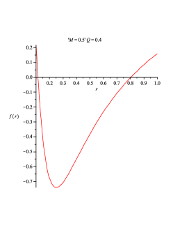
Figure 1: Event horizons occur at $r_{-}$ and $r_{+}$, where $f(r)$ cuts the $r$-axis, using suitable parameters. Here $M=0.5$ and $Q=0.4$.

The purpose of this paper is to employ this class of regular charged black holes to construct a traversable thin-shell wormhole by means of the cut-and-paste technique.

II Thin-Shell Wormhole Construction

The mathematical construction of our thin-shell wormhole begins by taking two copies of the regular charged black hole and removing from each the four-dimensional region

$$\Omega^{\pm}=\{r\leq a\,|\,a>r_{h}\}.$$

Here $r_{h}=r_{+}$, the larger of the two radii. We now identify (in the sense of topology) the timelike hypersurfaces

$$\partial\Omega^{\pm}=\{r=a\,|\,a>r_{h}\},$$

denoted by $\Sigma$. The resulting manifold is geodesically complete and consists of two asymptotically flat regions connected by a throat. The induced metric on $\Sigma$ is given by

$$ds^{2}=-d\tau^{2}+a(\tau)^{2}(d\theta^{2}+\sin^{2}\theta d\phi^{2}),$$ (4)

where $\tau$ is the proper time on the junction surface. Using the Lanczos equations Visser1989 ; Poisson1995 ; Lobo2003 ; Lobo2004 ; Eiroa2004a ; Eiroa2004b ; Eiroa2005 ; Thibeault2005 ; Lobo2005 ; Rahaman2006 ; Eiroa2007 ; Rahaman2007a ; Rahaman2007b ; Rahaman2007c ; Richarte2007 ; Lemos2008 ; Rahaman2008a ; Rahaman2008b ; Eiroa2008a ; Eiroa2008b ,

$$S^{i}_{\phantom{i}j}=-\frac{1}{8\pi}\left([K^{i}_{\phantom{i}j}]-\delta^{i}_{\phantom{i}j}[K]\right),$$

one can obtain the surface stress-energy tensor $S^{i}_{\phantom{i}j}=\text{diag}(-\sigma,p_{\theta},p_{\phi})$, where $\sigma$ is the surface-energy density and $p=p_{\theta}=p_{\phi}$ is the surface pressure. The Lanczos equations now yield

$$\sigma=-\frac{1}{4\pi}[K^{\theta}_{\phantom{\theta}\theta}]$$

and

$$p=\frac{1}{8\pi}\left([K^{\tau}_{\phantom{\tau}\tau}]+[K^{\theta}_{\phantom{\theta}\theta}]\right).$$

A dynamic analysis can be obtained by letting the radius $r=a$ be a function of time Poisson1995 . As a result,

$$\sigma=-\frac{1}{2\pi a}\sqrt{f(a)+\dot{a}^{2}}$$ (5)

and

$$p_{\theta}=p_{\phi}=p=-\frac{1}{2}\sigma+\frac{1}{8\pi}\frac{2\ddot{a}+f^{\prime}(a)}{\sqrt{f(a)+\dot{a}^{2}}}.$$ (6)

Here $p$ and $\sigma$ obey the conservation equation

$$\frac{d}{d\tau}(\sigma a^{2})+p\frac{d}{d\tau}(a^{2})=0$$ (7)

or

$$\dot{\sigma}+2\frac{\dot{a}}{a}(p+\sigma)=0.$$ (8)

In the above equations, the overdot and prime denote, respectively, the derivatives with respect to $\tau$ and $a$.

For a static configuration of radius $a$, we obtain (assuming $\dot{a}=0$ and $\ddot{a}=0$) from Eqs. (5) and (6)

$$\sigma=-\frac{1}{2\pi a}\left[1-\frac{2M}{a}+\frac{2M}{a}\tanh\left(\frac{Q^{2}}{2Ma}\right)\right]^{\frac{1}{2}}$$ (9)

and

$$p=\frac{\left[1-\frac{M}{a}+\frac{M}{a}\tanh\left(\frac{Q^{2}}{2Ma}\right)-\frac{Q^{2}}{2a^{2}}\cosh^{-2}\left(\frac{Q^{2}}{2Ma}\right)\right]}{4\pi a\left[1-\frac{2M}{a}+\frac{2M}{a}\tanh\left(\frac{Q^{2}}{2Ma}\right)\right]^{\frac{1}{2}}}.$$ (10)

Observe that the energy-density $\sigma$, as well as $\sigma+p$, are negative. So the shell contains matter that violates both the null energy condition (NEC) and the weak energy condition (WEC). Also, since $\sigma+2p$ and $\sigma+3p$ are positive, the strong energy condition is satisfied.
Using various values of the parameters $M$ and $Q$, Figures 2-9 show the plots for $\sigma$ and $p$ as functions of the radius $a$. We choose typical wormholes whose radii fall within the range 0.01 to 10 km.

III Equation of state

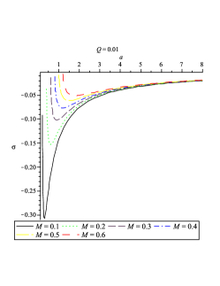
Figure 2: Plots for $\sigma$ versus $a$. We choose the fixed value $Q=0.01$ and various values for $M$.

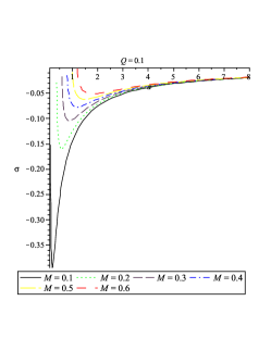
Figure 3: Plots for $\sigma$ versus $a$. We choose the fixed value $Q=0.1$ and various values for $M$.

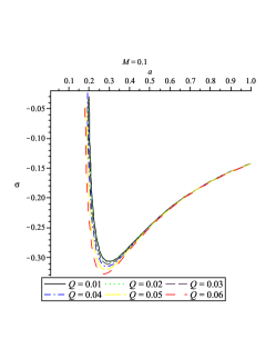
Figure 4: Plots for $\sigma$ versus $a$. We choose the fixed value $M=0.1$ and various values for $Q$.

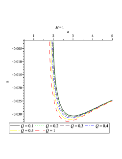
Figure 5: Plots for $\sigma$ versus $a$. We choose the fixed value $M=1$ and various values for $Q$.

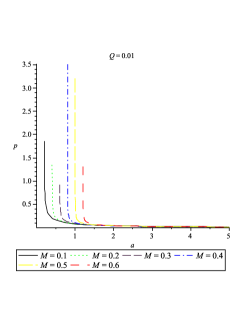
Figure 6: Plots for $p$ versus $a$. We choose the fixed value $Q=0.01$ and various values for $M$.

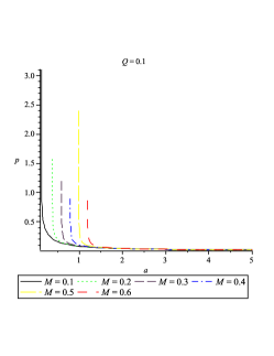
Figure 7: Plots for $p$ versus $a$. We choose the fixed value $Q=0.1$ and various values for $M$.

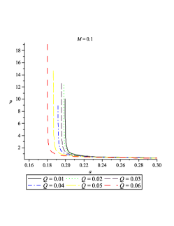
Figure 8: Plots for $p$ versus $a$. We choose the fixed value $M=0.1$ and various values for $Q$.

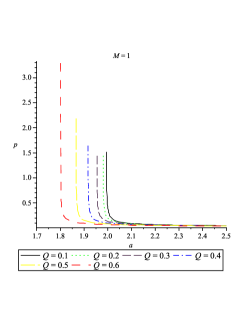
Figure 9: Plots for $p$ versus $a$. We choose the fixed value $M=1$ and various values for $Q$.

Let us suppose that the EoS at the surface $\Sigma$ is $p=w\sigma,w\equiv\text{constant}$. From Eqs. (9) and (10),

$$\frac{p}{\sigma}=w=\\ -\frac{1}{2}-\frac{M}{2a}\frac{\left[1-\tanh\left(\frac{Q^{2}}{2Ma}\right)-\frac{Q^{2}}{2Ma}\cosh^{-2}\left(\frac{Q^{2}}{2Ma}\right)\right]}{4\pi a\left[1-\frac{2M}{a}+\frac{2M}{a}\tanh\left(\frac{Q^{2}}{2Ma}\right)\right]}.$$ (11)

Observe that if $a\rightarrow\infty$, i.e., the location of the wormhole throat is large enough, then $w\rightarrow-\frac{1}{2}$. When $a\rightarrow a_{0}$, where $a_{0}$ is the point where the curve cuts the $a$-axis in Fig 10, then $p\rightarrow 0$, which would normally be viewed as a dust shell. Since $a_{0}<r_{h}$, however, the dust shell is never be found. On the other hand, since the Casimir effect with a massless field is of the traceless type, it may be of interest to check the traceless surface stress-energy tensor, $S^{i}_{\phantom{i}j}=0$, i.e., $-\sigma+2p=0$. From this equation we find that

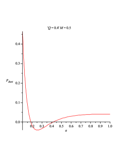
Figure 10: The curve cuts the $a$-axis at $a_{0}<r_{h}$; for the given plot, $M=0.5$ and $Q=0.4.$

.

$$g(a)\equiv 4-\frac{6M}{a}+\frac{6M}{a}\tanh\left(\frac{Q^{2}}{2Ma}\right)\\ -\frac{Q^{2}}{a^{2}}\cosh^{-2}\left(\frac{Q^{2}}{2Ma}\right)=0.$$ (12)

Figure 11 indicates that the value of $a$ satisfying this equation is inside the event horizon ($r=r_{h}$) of the regular black hole. It follows that this situation cannot arise in a wormhole setting.

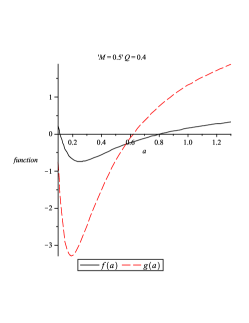
Figure 11: The curve $g(a)$ cuts the $a$-axis at a point less than $r_{h}$; for the given plot, $M=0.5$ and $Q=0.4$ .

IV The Gravitational field

In this section we are going to take a brief look at the attractive or repulsive nature of our wormhole. To do so, we calculate the observer’s four-acceleration

$$a^{\mu}=u^{\mu}_{;\nu}u^{\nu},$$

where

$$u^{\nu}=\frac{dx^{\nu}}{d{\tau}}=\left(\frac{1}{\sqrt{f(r)}},0,0,0\right).$$

Taking into account Eq. (2), the only nonzero component is given by

$$a^{r}=\Gamma^{r}_{tt}\left(\frac{dt}{d\tau}\right)^{2}=\frac{M}{r^{2}}\alpha(r),$$

where

$$\alpha(r)=\left[1-\tanh\left(\frac{Q^{2}}{2Mr}\right)-\frac{Q^{2}}{2Mr}\cosh^{-2}\left(\frac{Q^{2}}{2Mr}\right)\right].$$ (13)

A test particle moving radially from rest obeys the geodesic equation

$$\frac{d^{2}r}{d\tau^{2}}=-\Gamma^{r}_{tt}\left(\frac{dt}{d\tau}\right)^{2}=-a^{r}.$$

It is true in general that a wormhole is attractive whenever $a^{r}>0$. In our situation, $a^{r}$ is positive for $r>\frac{Q^{2}}{2Mr_{0}}$, where $r_{0}$ is the point where $\alpha(r)$ cuts the $x$-axis in Fig. 12. In other words, the wormhole is attractive for $r>\frac{Q^{2}}{2Mr_{0}}$ and repulsive for $r<\frac{Q^{2}}{2Mr_{0}}$. Finally, an observer at rest is a geodesic observer whenever $r=\frac{Q^{2}}{2Mr_{0}}$.

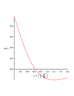
Figure 12: $r_{0}$ is the point where $\alpha(r)$ cuts the $x$-axis.

V The Total amount of exotic matter

In this section we determine the total amount of exotic matter for the thin-shell wormhole. This total can be quantified by the integral Eiroa2005 ; Thibeault2005 ; Lobo2005 ; Rahaman2006 ; Eiroa2007 ; Rahaman2007a ; Rahaman2007b

$$\Omega_{\sigma}=\int[\rho+p]\sqrt{-g}d^{3}x.$$ (14)

By introducing the radial coordinate $R=r-a$, w get

$$\Omega_{\sigma}=\int^{2\pi}_{0}\int^{\pi}_{0}\int^{\infty}_{-\infty}[\rho+p]\sqrt{-g}\,dR\,d\theta\,d\phi.$$

Since the shell is infinitely thin, it does not exert any radial pressure. Moreover, $\rho=\delta(R)\sigma(a)$. So

$$\Omega_{\sigma}=\int^{2\pi}_{0}\int^{\pi}_{0}\left.[\rho\sqrt{-g}]\right|_{r=a}d\theta\,d\phi=4\pi a^{2}\sigma(a)\\ =4\pi a^{2}\left(-\frac{1}{2\pi a}\right)\sqrt{1-\frac{2M}{a}+\frac{2M}{a}\text{tanh}\left(\frac{Q^{2}}{2Ma}\right)}\\ =-2a\sqrt{1-\frac{2M}{a}+\frac{2M}{a}\text{tanh}\left(\frac{Q^{2}}{2Ma}\right)}.$$ (15)

This NEC violating matter ($\Omega_{\sigma}$) can be reduced by choosing a value for $a$ closer to $r=r_{h}$. The closer $a$ is to $r_{h}$, however, the closer the wormhole is to a black hole: incoming microwave background radiation would get blueshifted to an extremely high temperature tR93 . On the other hand, it follows from Eq. (15) that for $a\gg r_{h}$, $\Omega_{\sigma}$ will depend linearly on $a$:

$$\Omega_{\sigma}\approx-2a.$$ (16)

The variation of the total amount of exotic matter with respect to the mass and charge of the black hole can best be seen graphically (Figures 13 - 15). Observe that the mass on the thin shell can be reduced by either increasing the mass or decreasing the charge of the black hole.

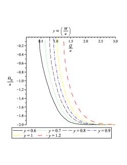
Figure 13: The variation in the total amount of exotic matter on the shell with respect to the charge of the black hole, while assuming a fixed mass for the black hole.

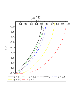
Figure 14: The variation in the total amount of exotic matter on the shell with respect to the mass of the black hole, while assuming a fixed charge for the black hole.

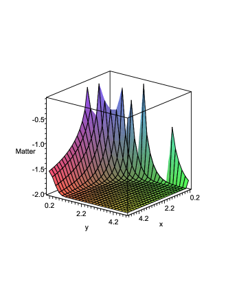
Figure 15: The variation in the total amount of exotic matter on the shell with respect to the mass ($x=\frac{M}{a}$) and the charge ($y=\frac{Q}{a}$) of the black hole.

VI Stability

In this section we turn to the question of stability of the wormhole using two different approaches: (i) assuming a specific equation of state on the thin shell and (ii) analyzing the stability to linearized radial perturbations.

VI.1 Reintroducing the equation of state

Suppose we return to the EoS

$$p=w\sigma,\quad w<0,$$ (17)

which is analogous to the equation of state normally associated with dark energy. Then Eq. (8) yields

$$\sigma(a)=\sigma_{0}\left(\frac{a_{0}}{a}\right)^{2(1+w)},$$ (18)

where $a=a_{0}$ is the static solution and $\sigma_{0}=\sigma(a_{0})$. Rearranging Eq. (5), we obtain the thin shell’s equation of motion

$$\dot{a}^{2}+V(a)=0.$$ (19)

Here the potential $V(a)$ is defined as

$$V(a)=f(a)-\left[2\pi a\sigma(a)\right]^{2}.$$ (20)

Substituting the value of $\sigma(a)$ in this equation, we obtain the following form of the potential:

$$V(a)=1-\frac{2M}{a}+\frac{2M}{a}\tanh\left(\frac{Q^{2}}{2Ma}\right)-\frac{A}{a^{2+4w}},$$ (21)

where $A=4\pi^{2}\sigma_{0}^{2}a_{0}^{4+4w}$.

If $-1<w<0$, then $p+\sigma=\sigma w+\sigma=\sigma(1+w)<0$, so that the WEC is violated. Figure 16 shows that the wormhole is stable for a certain range of parameters. (We will examine this range more closely in the next subsection.)

If $w<-1$, then $p+\sigma>0$. So the WEC is not violated and the collapse of the wormhole cannot be prevented (see Figure 17). In other words, if the exotic matter is removed, the wormhole will collapse.

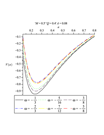
Figure 16: Wormholes are stable.

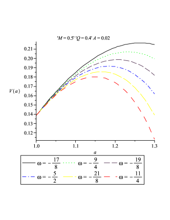
Figure 17: Wormholes are unstable.

VI.2 Linearized stability

Now we will focus our attention on the stability of the configuration under small perturbations around a static solution at $a=a_{0}$. Expanding $V(a)$ around $a_{0}$, we obtain

$$V(a) = V(a_{0})+V^{\prime}(a_{0})(a-a_{0})+\frac{1}{2}V^{\prime\prime}(a_{0})(a-a_{0})^{2}$$ (22)

$$+O\left[(a-a_{0})^{3}\right],$$

where the prime denotes the derivative with respect to $a$. Since we are linearizing around $a=a_{0}$, we require that $V(a_{0})=0$ and $V^{\prime}(a_{0})=0$. The configuration will be in stable equilibrium if $V^{\prime\prime}(a_{0})>0$. The subsequent analysis will depend on a parameter $\beta$, which is usually interpreted as the subluminal speed of sound and is given by the relation

$$\beta^{2}(\sigma)=\left.\frac{\partial p}{\partial\sigma}\right|_{\sigma}.$$

To that end, we start with Eq. (8) and deduce that $(a\sigma)^{\prime}=-(\sigma+2p)$. Also,

$$(a\sigma)^{\prime\prime}=-(\sigma^{\prime}+2p^{\prime})=-\sigma^{\prime}\left(1+2\frac{\partial p}{\partial\sigma}\right)\\ =2\left(1+2\frac{\partial p}{\partial\sigma}\right)\frac{\sigma+p}{a}=2(1+2\beta^{2})\frac{\sigma+p}{a}.$$

Returning to Eq. (20), we now obtain

$$V^{\prime}(a)=f^{\prime}(a)+8\pi^{2}a\sigma(\sigma+2p)$$

and

$$V^{\prime\prime}(a)=f^{\prime\prime}(a)-8\pi^{2}(\sigma+2p)^{2}\\ -8\pi^{2}[2\sigma(1+\beta^{2})(\sigma+p)].$$

When evaluating at the static solution $a=a_{0}$, we get the expected results $V(a_{0})=0$ and $V^{\prime}(a_{0})=0$. The stability condition $V^{\prime\prime}(a_{0})>0$ now yields the intermediate result

$$2\sigma(\sigma+p)(1+2\beta^{2})<\frac{f^{\prime\prime}(a_{0})}{8\pi^{2}}-(\sigma+2p)^{2}.$$ (23)

Since both $\sigma$ and $\sigma+p$ are negative, we retain the sense of the inequality to get

$$\beta^{2}<\frac{\frac{f^{\prime\prime}(a_{0})}{8\pi^{2}}-(\sigma+2p)^{2}-2\sigma(\sigma+p)}{2[2\sigma(\sigma+p)]}.$$ (24)

It follows that there is only one region of stability. Substituting for $\sigma$ and $p$ results in

$$\beta^{2}<\frac{1}{2(a_{0}f_{0}^{\prime}-2f_{0})}\left[a_{0}f_{0}^{\prime}-2f_{0}-a_{0}^{2}f_{0}^{\prime\prime}+\frac{a_{0}^{2}(f_{0}^{\prime})^{2}}{2f_{0}}\right]-1;$$ (25)

here $f_{0}=f(a_{0})$, $f^{\prime}_{0}=f^{\prime}(a_{0})$, and $f^{\prime\prime}_{0}=f^{\prime\prime}(a_{0})$. The final step is to substitute the expressions for $f_{0}$, $f^{\prime}_{0}$, and $f^{\prime\prime}_{0}$ and to graph the result for various values of the parameters to obtain the region of stability (below the curve in each case). According to Figures 18 and 19, stable solutions exist for a wide range of parameters.

Returning to Figure 16 in the previous subsection, if $-1<w<0$, then $\sigma(\sigma+p)>0$ and the inequality in (23) is preserved, leading to criterion (24). The parametric values $M=0.5$ and $Q=0.4$ do indeed lie in the stability region, according to Figure 18.

For $w<-1$ in Figure 17, $\sigma(\sigma+p)<0$, so that the sense of the inequality in (23) is not preserved, taking us out of the region of stability.

As noted earlier, since one normally interprets $\beta$ as the speed of sound, the value should not exceed 1. According to Figures 18 and 19, this requirement is met in the region of stability. The result makes an interesting contrast to the wormhole in Ref. Poisson1995 , constructed by using two copies of Schwarzschild spacetime. For that wormhole there are two separate regions of stability that do not include the values $0<\beta^{2}\leq 1$, i. e., the wormhole is unstable for all values of $a_{0}$ whenever $\beta$ is in this range.

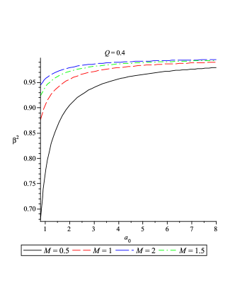
Figure 18: Stability region is given below the curve.

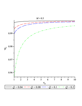
Figure 19: Stability region is given below the curve.

VII Conclusions

This paper investigates a new thin-shell wormhole constructed by applying the cut-and-paste technique to two regular charged black-hole spacetimes first introduced by Beato and Garcia. The construction allows a graphical description of both $\sigma$ and $p$ as functions of the radius $a$ of the thin shell, using various values of the mass $M$ and the charge $Q$. The same parameters help determine whether the wormhole is attractive or repulsive. Finally, the total amount of exotic matter required is determined both analytically and graphically.

The issue of stability is addressed in two ways: first by assuming the EoS $p=w\sigma$, $w<0$, on the thin shell and then by analyzing the stability to linearized radial perturbations. The latter yields a single region of stability covering a wide range of values of the parameters $M,Q,$ and $a=a_{0}$. The region includes the stable solutions that depend on the EoS $p=w\sigma$.

For our wormhole, the parameter $\beta$, which is normally interpreted as the speed of sound, has the desired values $0<\beta^{2}\leq 1$, unlike the wormholes constructed from two Scharzschild spacetimes Poisson1995 . These are unstable for all values of $a=a_{0}$ in this range.

References

- (1) M. Visser, Nucl. Phys. B 328, (1989) 203.
- (2) E. Poisson and M. Visser, Phys. Rev. D 52, (1995) 7318.
- (3) F.S.N. Lobo and P. Crawford, Class. Quant. Grav. 21, (2004) 391.
- (4) F.S.N. Lobo, Class. Quant. Grav. 21, (2004) 4811.
- (5) E.F. Eiroa and G. Romero, Gen. Rel. Grav. 36, (2004) 651.
- (6) E.F. Eiroa and C. Simeone, Phys. Rev. D 70, (2004) 044008.
- (7) E.F. Eiroa and C. Simeone, Phys. Rev. D 71, (2005) 127501.
- (8) M. Thibeault, C. Simeone, and E.F. Eiroa, Gen. Rel. Grav. 38, (2006) 1593.
- (9) F.S.N. Lobo, Phys. Rev. D 71, (2005) 124022.
- (10) F. Rahaman et al., Gen. Rel. Grav. 38, (2006) 1687.
- (11) E.F. Eiroa and C. Simeone, Phys. Rev. D 76, (2007) 024021.
- (12) F. Rahaman et al., Int. J. Mod. Phys. D 16, (2007) 1669.
- (13) F. Rahaman et al., Gen. Rel. Grav. 39, (2007) 945.
- (14) F. Rahaman et al., Chin. J. Phys. 45, (2007) 518 arXiv:0705.0740 [gr-qc]
- (15) M. G. Richarte and C. Simeone, Phys. Rev. D 76, (2007) 087502.
- (16) J. P. S. Lemos and F.S.N. Lobo, Phys. Rev D 78, (2008) 044030.
- (17) F. Rahaman et al., Acta Phys. Polon. B 40 , ( 2009 ) 1575 arXiv: gr-qc/0804.3852.
- (18) F. Rahaman et al., Mod. Phys. Lett. A 24, (2009) 53 arXiv: gr-qc/0806.1391.
- (19) E.F. Eiroa, Phys. Rev. D 78, (2008) 024018.
- (20) E.F. Eiroa, M.G. Richarte, and C. Simeone, Phys. Lett. A 373 (2008) 1.
- (21) E. A. Beato and A. García, Phys. Lett. B 464, (1999) 25.
- (22) T.A. Roman, Phys. Rev. D 53, (1993) 5496.