Analysis of the Laplacian and Spectral Operators on the Vicsek Set

Abstract.

We study the spectral decomposition of the Laplacian on a family of fractals $\mathcal{VS}_{n}$ that includes the Vicsek set for $n=2$, extending earlier research on the Sierpinski Gasket. We implement an algorithm [24] for spectral decimation of eigenfunctions of the Laplacian, and explicitly compute these eigenfunctions and some of their properties. We give an algorithm for computing inner products of eigenfunctions. We explicitly compute solutions to the heat equation and wave equation for Neumann boundary conditions. We study gaps in the ratios of eigenvalues and eigenvalue clusters. We give an explicit formula for the Green’s function on $\mathcal{VS}_{n}$. Finally, we explain how the spectrum of the Laplacian on $\mathcal{VS}_{n}$ converges as $n\to\infty$ to the spectrum of the Laplacian on two crossed lines (the limit of the sets $\mathcal{VS}_{n}$.)

1. Introduction

Kigami [16] has developed a theory of Laplacians on a class of fractals called pcf self-similar fractals. One example, the Sierpinski gasket $\mathcal{SG}$ has become the “poster child” for this theory [22] in the belief that it is the simplest nontrivial example. As a result, a lot of very concrete results have been obtained for $\mathcal{SG}$. This paper extends some of these concepts and results to a different family of finitely ramified self-similar fractals, the Vicsek sets $\mathcal{VS}_{n}$, with $n=2$ corresponding to the Vicsek set $\mathcal{VS}$. We also obtain results for $\mathcal{VS}$ that have no analogs on $\mathcal{SG}$.

To review the standard theory, a pcf self-similar fractal $V$ will be a compact set in the plane, defined as the limit of a sequence of graphs $\Gamma_{0},\Gamma_{1},\ldots$ with vertices $V_{0}\subset V_{1}\subset\cdots$. The property of self-similarity takes the form of a family of mappings from $V$ to itself, $\{F_{i}\}$ which are contractive similarities and have the property that $V=F_{0}(V)\cup F_{1}(V)\cup\cdots\cup F_{k}(V)$. For example, the Sierpinski Gasket is defined by three similarities, each of which sends the entire set $\mathcal{SG}$ to one of its three smaller triangular component copies. We refer to the graph at stage $m$ of the approximation as the $m$th level graph approximation. The Vicsek set (specifically the second order Vicsek set $\mathcal{VS}_{2}$, but sometimes simply called the Vicsek set) is the fractal defined by the similarities $F_{i}\colon\mathcal{VS}_{2}\to\mathcal{VS}_{2}$

$$F_{1}(x) =x/3 F_{4}(x) =x/3+2/3(0,1)$$

$$F_{2}(x) =x/3+2/3(1,0) F_{0}(x) =x/3+2/3(1/2,1/2)$$

$$F_{3}(x) =x/3+2/3(1,1)$$

The first graph approximation $\Gamma_{0}$ is the complete graph on four vertices (that is, the vertices of a unit square and an edge connecting every pair of vertices). The next approximation $\Gamma_{1}$ consists of five miniature copies of $\Gamma_{0}$ arranged in an X shape with branches of length 2 (hence $\mathcal{VS}_{2}$). Further graph approximations likewise consist of five copies of the previous level; they display finer levels of branching.

Figure 1. $\mathcal{VS}_{2}$

Figure 2. $\mathcal{VS}_{3}$

Higher order Vicsek sets $\mathcal{VS}_{n}$ are similar, except that $\Gamma_{1}$ is an X-shaped graph consisting not of five but $4n-3$ copies of $\Gamma_{0}$, with arms of length $n$. Instead of five similarities, we have $4n-3$ similarities.

It is intuitive from the picture and also easy to demonstrate that as $n\to\infty$, $\mathcal{VS}_{n}$ approaches the pair of crossed line segments between $(0,0)$ and $(1,1)$ and $(1,0)$ and $(0,1)$. (That is, the maximum Euclidean distance of any point in $\mathcal{VS}_{n}$ from the crossed lines approaches zero.) This is important to note because it suggests a connection between fractal analysis on the Vicsek sets and classical analysis on the line; later in this paper we show that the spectrum of the (Neumann) Laplacian as defined on the Vicsek sets does, in fact, approach the spectrum for the classical Neumann Laplacian on the cross.

On $\mathcal{VS}_{n}$, we can define a standard self-similar probability measure as follows: for each graph approximation, let $\nu_{m}$ be the probability measure which weights each vertex by its degree. Then the standard measure $\mu$ on $\mathcal{VS}_{n}$ is defined by

$$\int_{\mathcal{VS}_{2}}fd\mu=\lim_{m\to\infty}\int_{\Gamma_{m}}fd\nu_{m}.$$

We define the unrenormalized energy of a function on $\Gamma_{m}$ by

$$E_{m}(u)=\sum_{x\sim y}|u(x)-u(y)|^{2}.$$

The renormalization factor for $\mathcal{VS}_{n}$ is $2n-1$, so the renormalized graph energy on $\Gamma_{m}$ is

$$\mathcal{E}_{m}(u)=(2n-1)^{-m}E_{m}(u),$$

and we can define the fractal energy $\mathcal{E}(u)=\lim_{m\to\infty}\mathcal{E}_{m}(u)$. We define $\mathop{\mathrm{dom}}\mathcal{E}$ as the space of continuous functions with finite energy.

Now we have the tools to define a fractal Laplacian. In $\mathop{\mathrm{dom}}\mathcal{E}$, $\mathcal{E}$ extends by the polarization formula to a bilinear form $\mathcal{E}(u,v)$ which defines an inner product in this space. If $\mu$ is the standard measure, we can define the Laplacian with a weak formulation: $\Delta u=f$ if $f$ is continuous, $u\in\mathop{\mathrm{dom}}\mathcal{E}$, and

$$\mathcal{E}(u,v)=-\int fv\,d\mu\qquad\forall v\in\textstyle\mathop{\mathrm{dom}}_{0}\mathcal{E}$$

where $\mathop{\mathrm{dom}}_{0}\mathcal{E}=\{v\in\mathcal{E}:v|_{\rm bdry}=0\}$. There is also a pointwise formula (which is proven to be equivalent in [22]) which, for nonboundary points in $\mathcal{VS}_{n}$ computes

$$\Delta u(x)=\lim_{m\to\infty}K(4n-3)^{m}(2n-1)^{m}\Delta_{m}u(x),$$

with $K$ a constant, and where $\Delta_{m}$ is a discrete Laplacian associated with the graph $\Gamma_{m}$, defined by

$$\Delta_{m}u(x)=\frac{1}{\mathop{\text{deg}}x}\sum_{y\sim x}(u(y)-u(x)),\qquad\text{for $x$ not on the boundary}.$$

The Laplacian satisfies the scaling property

$$\Delta(u\circ F_{i})=(4n-3)(2n-1)(\Delta u)\circ F_{i}$$

and by iteration

$$\Delta(u\circ F_{w})=\big{(}(4n-3)(2n-1)\big{)}^{m}(\Delta u)\circ F_{w}$$

for $F_{w}=F_{w_{1}}\circ F_{w_{2}}\circ\cdots\circ F_{w_{m}}$.

In this paper, we restrict attention to the Laplacian defined with Neumann boundary conditions. The Neumann boundary conditions are “natural”, in the sense that the weak formulation need only be modified to allow all $v\in\mathop{\mathrm{dom}}\mathcal{E}$, and the pointwise formulation is also valid at boundary points. It is also possible to define a normal derivative $\partial_{n}u(q_{i})$ at boundary point, and the Neumann condition is $\partial_{n}u(q_{i})=0$. Moreover, there are infinitely many points in $\mathcal{VS}_{n}$ that have neighborhoods isometric to neighborhoods of boundary points; the Neumann boundary conditions treat the boundary points no differently from these equivalent points. (Note that this is not true on $\mathcal{SG}$.) These are ample reasons to prefer Neumann to Dirichlet boundary conditions. An additional benefit is that the theory is considerably simpler.

The Laplacian on a fractal such as $\mathcal{SG}$ or $\mathcal{VS}_{n}$ has a discrete spectrum of positive eigenvalues $\lambda_{0}<\lambda_{1}<\lambda_{2}<\cdots$, which can be computed explicitly by the method of spectral decimation developed by Fukushima and Shima, and applied to the Vicsek set in [24]. Spectral decimation is a method of relating eigenfunctions and eigenvalues from one graph approximation to a finer one. In Section 2, we describe the method and explicitly compute an algorithm for spectral decimation on $\mathcal{VS}_{2}$, which allows us to numerically calculate eigenfunctions on the Vicsek set, and observe patterns in the data.

Let $\{\lambda_{j}\}$ denote the spectrum of the Laplacian, and let $\{u_{j}\}$ denote an orthonormal basis of eigenfunctions. Then for any bounded function $f$, we can define the spectral operator $f(-\Delta)$ on $L^{2}(\mathcal{VS}_{n})$ by

$$f(-\Delta)u=\sum_{j=1}^{\infty}f(\lambda_{j})\langle u,u_{j}\rangle u_{j}.$$

These operators include the fundamental solutions to the heat and wave equations, and solutions for other space-time equations. Because of the importance of spectral operators to classical analysis, understanding spectral operators and the Laplacian on $\mathcal{VS}$ is a key goal in the development of analysis on fractals.

In computing a spectral operator, we can group terms in the sum corresponding to the same eigenvalue, and write

$$f(-\Delta)u(x)=\sum_{\lambda_{j}}f(\lambda)\int P_{\lambda}(x,y)u(y)d\mu(y)$$

where, at a given point $x$

$$P_{\lambda}(x,y)=\sum_{j}u_{j}(x)u_{j}(y),$$

$\{u_{j}\}$ being an orthonormal basis of the $\lambda$-eigenspace $E_{\lambda}$. In Section 3 we show how, for certain special points $x$, we can simplify this sum to a single term. Fixing a point $x$ on the boundary, or at the center, and letting $E_{\lambda}^{x}$ denote the subspace of $E_{\lambda}$ of functions vanishing at $x$, we can choose the orthonormal basis so that the first element $u_{1}$ is in $(E_{\lambda}^{x})^{\perp}$ and the rest belong to $E_{\lambda}^{x}$. Then,

$$P_{\lambda}(x,y)=u_{1}(x)u_{1}(y).$$

Additionally, in Section 3 we prove a formula for the inner product of two eigenfunctions on a graph approximation, and show that it converges in the limit to the inner product on the Vicsek set. This ensures that functions which are orthogonal on graph approximations remain orthogonal on the Vicsek set, and makes it possible to compute $P_{\lambda}$ when $x$ is a point on the boundary or at the center. Here we follow some of the ideas in [2].

In Section 4, we give some numerical data using our MATLAB algorithms for the eigenvalues and eigenfunctions of the Laplacian on $\mathcal{VS}_{2}$ and $\mathcal{VS}_{n}$. We also give data on the eigenvalue counting function $N(x)$ and the Weyl ratio $N(x)/x^{\alpha}$, for the appropriate power $\alpha$.

In Section 5, we give numerical results for the heat kernel, the propagator for the wave equation, and the spectral projections onto the 0-series.

In Section 6, we show that each 0-series eigenfunction is determined by its restriction to the diagonal of the Vicsek set.

In Section 7, we prove, following [5] the existence of a ratio gap in the spectrum of the Laplacian. A ratio gap is an interval $(a,b)$ such that the ratio of any two eigenvalues must fall outside the interval; this is a measure of the sparseness of the spectrum. Related results have been obtained in [15].

In Section 8, we show the existence of eigenvalue clusters; that is, arbitrarily many distinct eigenvalues in an arbitrarily small interval.

In Section 9, we calculate an explicit Green’s function for the Laplacian on the Vicsek set.

In Section 10, we examine the convergence of eigenfunctions and eigenvalues of the Laplacian on $\mathcal{VS}_{n}$ as $n\to\infty$ and show that they approach the corresponding values for the Laplacian on the cross.

In Section 11 we establish some properties of the Weyl ratio on $\mathcal{VS}_{n}$ that begin to explain the curious apparent convergence to a function that is unrelated to the Weyl ratio on the cross.

For more data and programs, refer to www.math.cornell.edu/~mhw33 ([7]).

It is possible to describe $\mathcal{VS}_{n}$ as the closure of a countable union of straight line segments; start with the two diagonals, and take all images under all iterates of $\{F_{i}\}$. (Some images will be proper subsets of other line segments and should be deleted to eliminate redundancy.) We call this the skeleton of $\mathcal{VS}_{n}$, $SK(\mathcal{VS}_{n})=\cup_{j=1}^{\infty}I_{j}$, where the line segments $I_{j}$ intersect only at points. Since the skeleton is dense, any continuous function is uniquely determined by its restriction to the skeleton, but the skeleton is not all of the Vicsek set, since it has $\mu$-measure zero.

Each line segment $I_{j}$ has a simple one-dimensional energy

$$\mathcal{E}_{j}(u,v)=\int_{-b_{j}}^{b_{j}}u^{\prime}(s_{j}(t))v^{\prime}(s_{j}(t))dt$$

where $s_{j}:[-b_{j},b_{j}]\to I_{j}$ is the linear parametrization. It is not difficult to see that

$$\mathcal{E}(u,v)=c\sum_{j=1}^{\infty}\mathcal{E}_{j}(u|_{I_{j}},v|_{I_{j}})$$

for the appropriate constant $c$. From this point of view, the energy form on $\mathcal{VS}_{n}$ is trivial. Because we combine the trivial energy with the unrelated measure $\mu$, we obtain a nontrivial Laplacian.

On the other hand, there is a natural measure on the skeleton: just take the sum of Lebesgue measure on each $I_{j}$. By the embedding of the skeleton in $\mathcal{VS}_{n}$ we may also regard this as a measure $\nu$ on $\mathcal{VS}_{n}$. Of course it is not a finite measure, as the sum of the lengths of the line segments $I_{j}$ diverges. It satisfies the self-similar identity

$$\nu=\frac{1}{2n-1}\sum_{i}\nu\circ F_{i}^{-1}$$

in contrast to the self-similar identity

$$\mu=\frac{1}{4n-3}\sum_{i}\mu\circ F_{i}^{-1}$$

for $\mu$. There is good reason to consider $\nu$ as the universal energy measure on $\mathcal{VS}_{n}$. If $f\in\mathop{\mathrm{dom}}\mathcal{E}$ then we may define an associated energy measure $\nu_{f}$ with $\mathcal{E}(f,f)=\nu_{f}(\mathcal{VS}_{n})$ and roughly speaking $\nu_{f}(A)$ is the contribution to $\mathcal{E}(f,f)$ coming from the set $A$, for any simple set $A$ (for example, a finite union of cells.) For each $I_{j}$ consider the function $f_{j}$ defined by $f_{j}(s_{j}(t))=t$ on $I_{j}$, which is constant on every other interval that intersects $I_{j}$. Then $f_{j}$ is harmonic at every point except the endpoints of $I_{j}$, and $\nu_{f_{j}}$ is exactly Lebesgue measure on $I_{j}$. So

$$\nu=\sum_{j=1}^{\infty}\nu_{f_{j}}.$$

We can also see that $f=\sum_{j=1}^{\infty}f_{j}$ is a finite sum on each $I_{j}$ and $\nu=\nu_{f}$, although $f$ does not have finite energy. One can also show that $\nu_{f}\ll\nu$ for every function $f\in\mathop{\mathrm{dom}}\mathcal{E}$. This is the “universal” property of $\nu$.

On $\mathcal{SG}$ one can define the Kusuoka measure $\nu=\nu_{h_{1}}+\nu_{h_{2}}$ where $\{h_{1},h_{2}\}$ is an orthonormal basis of global harmonic functions (modulo constants) in the energy norm, and this serves as a universal energy measure. A similar approach would not work on $\mathcal{VS}_{n}$, since it would produce a measure supported on the two diagonals alone.

It is possible to define an energy Laplacian on $\mathcal{VS}_{n}$ using the energy $\mathcal{E}$ and the energy measure $\nu$ in place of $\mu$, although there are some technical problems because $\nu$ is not finite. Such a Laplacian would be rather “trivial”, since it would amount to the second derivative along each line segment $I_{j}$, together with matching conditions on first derivatives at points of intersection. We will not consider this Laplacian further in this paper.

We hope that this paper makes a strong case that the Vicsek sets deserve to be considered the simplest nontrivial examples of pcf self-similar fractals. There are two sides to this statement. The first is that the analysis is nontrivial. Indeed, if you just restrict attention to harmonic functions on $\mathcal{VS}_{n}$, the theory is basically trivial: these are just linear functions on each of the arms of $\mathcal{VS}_{n}$ that are constant on all trees that attach to an arm. But the graphs we have obtained for eigenfunctions of the Laplacian reveal that these are nontrivial functions.

The other side of our assertion is that $\mathcal{VS}_{n}$ is simpler than $\mathcal{SG}$. The expression for the Green’s function and the numerical data for solutions of the wave equation are good a posteriori evidence for this. We can also point to two structural features that can be considered a priori evidence. The first is topological: $\mathcal{VS}_{n}$ is contractible while $\mathcal{SG}$ has infinite dimensional homology. Indeed, the cycles in $\mathcal{SG}$ play a role in the description of the structure of some of the eigenspaces of the Laplacian (the 5-series in the terminology of [22].) The second relates to symmetry: while $\mathcal{SG}$ only has a 6-element symmetry group, $\mathcal{VS}_{n}$ has an infinite symmetry group. Indeed this group is a semidirect product of one copy of $S_{4}$ and infinitely many copies of $S_{3}$ and $S_{2}$. ($S_{k}$ denotes the permutation group on $k$ letters.) The $S_{4}$ symmetries are the permutations of the 4 arms, which fix the center point $q_{0}$. For any cell, $F_{w}V$ with center point $F_{w}q_{0}$, with $w_{m}\neq 0$, there will be either $S_{2}$ or $S_{3}$ symmetries permuting 2 or 3 of the arms of the cell, depending on whether the cell $F_{w}V$ has 2 or 1 neighboring cells (the permutable arms are the ones with no neighbors.)

2. Spectral Decimation

The method of spectral decimation was invented by Fukushima and Shima [12] for $\mathcal{SG}$ to relate eigenfunctions and eigenvalues on the graph approximations to each other and the eigenfunctions and eigenvalues on $\mathcal{SG}$. In essence, an eigenfunction on $\Gamma_{m}$ with eigenvalue $\lambda_{m}$ can be extended to an eigenfunction on $\Gamma_{m+1}$ with eigenvalue $\lambda_{m+1}$, where $\lambda_{m}=R(\lambda_{m+1})$ for an explicit functions $R$, except for certain specified forbidden eigenvalues, and all eigenfunctions on $\mathcal{SG}$ arise as limits of this process starting at some level $m$. This is true regardless of the boundary conditions, but if we specify Dirichlet or Neumann boundary conditions we can describe explicitly all eigenspaces and their multiplicities. This method was extended to the Vicsek sets by Zhou [24].

We describe the procedure briefly here. First, there is a local extension algorithm that shows how to uniquely extend an eigenfunction $u$ defined on $V_{m}$ to a function defined on $V_{m+1}$ such that the $\lambda$-eigenvalue equations hold on all points of $V_{m+1}\setminus V_{m}$. Then there is a rational function $R(\lambda)$ such that if $u$ satisfies a $\lambda_{m}$-eigenvalue equation on $V_{m}$, then the extended function will satisfy the $\lambda_{m+1}$-eigenvalue equation on $V_{m+1}$ if $\lambda_{m}=R(\lambda_{m+1})$ and $\lambda_{m}$ is not a forbidden eigenvalue. (Forbidden eigenvalues are singularities of the spectral decimation function $R$. It is “forbidden” to decimate to a forbidden eigenvalue. Because forbidden eigenvalues have no predecessor — there is no $\lambda_{m-1}$ corresponding to $\lambda_{m}$ — we speak of forbidden eigenvalues being “born” at a level of approximation $m$.)

We have the following theorem from [24]:

Theorem 2.1.

Define

$$f_{n}(\lambda) =T_{n}(3\lambda-1)-3T_{n-1}(3\lambda-1)$$

$$g_{n}(\lambda) =U_{n-1}(3\lambda-1)-U_{n-2}(3\lambda-1)$$

$$h_{n}(\lambda) =U_{n-1}(3\lambda-1)-3U_{n-2}(3\lambda-1)$$

where $T_{n}$ and $U_{n}$ are the Chebyshev polynomials of the first and second kind. Then the spectral decimation function $R$ is

$$R(\lambda_{m})=\lambda_{m-1}=\lambda_{m}g_{m}(\lambda_{m})h_{m}(\lambda_{m}).$$

Moreover, the forbidden eigenvalues are 4/3 and the zeroes of $f_{n}$ and $g_{n}$.

We also have a matrix equation for the eigenfunction extension formula: If $u|_{V_{0}}$ is a vector of the values of $u$ on $V_{0}$ and $u|_{V_{1}\setminus V_{0}}$ is defined analogously, then

$$u|_{V_{1}\setminus V_{0}}=-(X+\lambda_{1}M)^{-1}Ju_{V_{0}}.$$

where $J$ is the $V_{0}\times(V_{1}\setminus V_{0})$ adjacency matrix, $X$ is the adjacency matrix for $V_{1}\setminus V_{0}$, with the degrees of each vertex as its diagonal entries, and $M$ is a diagonal matrix with $M_{ii}=-X_{ii}$. Multiplying this matrix by the values of $u$ on any $k$-cell (with $\lambda_{1}$ replaced by $\lambda_{k+1}$), we similarly get the values of $u$ on the $(k+1)$-cells contained in that $k$-cell.

In the case of $\mathcal{VS}_{2}$, we have $R(\lambda)=36\lambda^{3}-48\lambda^{2}+15\lambda$. The forbidden eigenvalues are $0$, $1/2$, $4/3$, and $(7\pm\sqrt{17})/12$. There is a 0-eigenvalue born at level 0, and a 4/3 eigenvalue born at every level thereafter, and continued eigenvalues are formed by successively choosing one of the three inverse functions of $R$ (see Figure 3), so long as this does not lead to a forbidden eigenvalue.

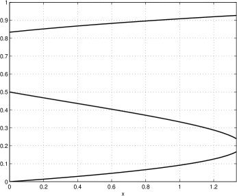
Figure 3. Inverse functions on $\mathcal{VS}_{2}$.

Using the labeling system described in Figure 4, the

Figure 4. Labeling system for the vertices $V_{1}$ of the first level graph approximation to $\mathcal{VS}_{2}$.

matrix which allows us to continue eigenfunctions is given by

(2.5) $$-(X+\lambda M)^{-1}J=\gamma\left(\begin{array}[]{cccccccccccc}a&b&a&c&c&d&d&c&c&c&d&c\\ c&d&c&a&a&b&d&c&c&c&d&c\\ c&d&c&c&c&d&b&a&a&c&d&c\\ c&d&c&c&c&d&d&c&c&a&b&a\end{array}\right)^{\top}$$

where

(2.6) $$\begin{aligned} a&=9-42\lambda+36\lambda^{2},&c&=1,\\ b&=6(1-4\lambda+3\lambda^{2}),&d&=2-3\lambda,\\ \gamma&=\frac{1}{3(4-29\lambda+60\lambda^{2}-36\lambda^{3})},\end{aligned}$$

(Note that only roots of $-3/\gamma=(1-2\lambda)f(\lambda)$ are forbidden eigenvalues, so $\gamma$ is well-defined as long as $\lambda$ is not forbidden.)

We denote the 4/3-series as those eigenvalues continued from a 4/3-eigenvalue, and the 0-series as those eigenvalues continued from the 0-eigenvalue. To find $\lambda_{m}$ from $\lambda_{m-1}$ we have to invert $R$; in the case of $\mathcal{VS}_{2}$, there are three inverses, shown in Figure 3. Note that for the sequence $15^{m}\lambda_{i}$ to converge to an eigenvalue $\lambda$ on $\mathcal{VS}$, we need $\lambda_{m}$ to approach zero, so we must choose the smallest of the three inverses all but finitely many times.

A proof in [24] guarantees that spectral decimation produces all possible eigenvalues and eigenfunctions (up to linear combination), so this formula allows us to explicitly determine the values of eigenfunctions at arbitrarily high graph approximations. We make several observations from numerical calculation of the eigenfunctions (see Section 6). One is that the restrictions of certain eigenfunctions to the diagonal (the segment in $\mathbb{R}^{2}$ between (0, 0) and (1, 1)) are periodic with period proportional to $1/m$ and approximate sine functions; this suggests that higher Vicsek sets $\mathcal{VS}_{n}$, as they converge to a cross, will have eigenfunctions approaching the sine and cosine functions in the classical case. We will prove this fact in Section 10.

Secondly, we observe that for the 0-series eigenfunctions, choosing the smallest inverse function of $R$ first means that $\lambda_{1}=0$ so the eigenfunction is extended to be constant on $V_{1}$. On each of the five 1-cells, we start as before, with the eigenfunction having a value of 1 one all boundary points; so the eigenfunction is miniaturized into identical copies at each graph approximation, and the eigenvalue is multiplied by 15. The same thing happens for any number of initial choices of the smallest inverse function.

We next describe the structure of the spectrum of the Neumann Laplacian on $\mathcal{VS}_{n}$ in complete detail. Let $\phi_{1},\phi_{2},\ldots,\phi_{2n-1}$ denote the inverse functions of the polynomial $R$ in Theorem 2.1, in increasing order. We note that $\phi_{j}$ is an increasing function when $j$ is odd and is a decreasing function when $j$ is even. We write $\rho_{n}=(4n-3)(2n-1)$ for the Laplacian renormalization factor. We write $0=\lambda_{0}<\lambda_{1}<\lambda_{2}<\cdots$ for the distinct eigenvalues. The spectral decimation rules are summarized as follows:

1. Each eigenvalue has the form

   $$\lim_{m\to\infty}\rho_{n}^{m}\phi_{w_{m}}\circ\phi_{w_{m-1}}\circ\cdots\circ\phi_{w_{1}}(0),$$

    or $$\lim_{m\to\infty}\rho_{n}^{m+k}\phi_{w_{m}}\circ\phi_{w_{m-1}}\circ\cdots\circ\phi_{w_{1}}(4/3).$$

   where in the first case the eigenvalue is in the 0-series and in the second case it is in the 4/3-series and born on level $k$.

2. All but a finite number of the $w_{m}$ are equal to 1.

3. For the 0-series, the first $w_{j}$ with $w_{j}\neq 1$ must have $w_{j}$ an odd number; for the 4/3-series, $w_{1}$ must be an odd number but $w_{1}\neq 2n-1$.

4. The multiplicity of each 0-series eigenvalue is 1, while the multiplicity of each 4/3-series eigenvalue born on level $k$ is $2(4n-3)^{k}+1$.

Condition (ii) is required in order that the limits in (i) exist. Let $m_{0}$ denote the largest value of $m$ for which $w_{m}\neq 1$ (if this never happens, let $m_{0}=0$.) Then we can rewrite the limits in (i) in terms of a single function $\psi_{n}$ defined by

$$\psi_{n}(t)=\lim_{m\to\infty}\rho_{n}^{m}\phi_{1}^{(m)}(t)$$

(here $\phi_{1}^{(m)}$ denotes the $m$-fold composition of $\phi_{1}$). This limit exists because the Taylor expansion of $R(t)$ about $t=0$ is $\rho_{n}t+O(t^{2})$, so the Taylor expansion of $\phi_{1}(t)$ about $t=0$ is $\rho_{n}^{-1}t+O(t^{2})$. Then (i) says the eigenvalues are either

$$\rho_{n}^{m_{0}}\psi_{n}(\phi_{w_{m_{0}}}\circ\phi_{w_{m_{0}-1}}\circ\cdots\circ\phi_{w_{1}}(0)),$$

 or $$\rho_{n}^{m_{0}+k}\psi_{n}(\phi_{w_{m_{0}}}\circ\phi_{w_{m_{0}}-1}\circ\cdots\phi_{w_{1}}(4/3)).$$

Condition (iii) spells out explicitly the rules for avoiding forbidden eigenvalues. We may explain the multiplicities in (iv) as follows. To satisfy the 4/3-eigenvalue equation on level $k$ we may assign initial values at the points in $V_{k}$ so that the sum of the values on the four boundary points of every $k$-cell is 0. This gives a space of dimension $\#\{V_{k}\}-\#\{k\text{-cells}\}$ and it is easy to see that $\#(V_{k})=3(4n-3)^{k}+1$ and $\#\{k\text{-cells}\}=(4n-3)^{k}$.

Theorem 2.2.

Eigenvalues in the 0-series and 4/3-series alternate: $\lambda_{j}$ is 0-series for $j$ even and 4/3-series for $j$ odd. More precisely, the spectrum consists of an initial segment of length $2n$ followed by segments of length $4n-2$. In each segment all the 4/3-series eigenvalues are born level 0 (hence have multiplicity 3) except the last one.

Proof.

Because $\phi_{1}$ is increasing, so is $\psi_{n}$, so applying $\psi_{n}$ does not change the order of eigenvalues. Thus the ordering of the eigenvalues can be inferred from the ordering and increasing/decreasing nature of the $\phi_{j}$’s. The lowest eigenvalues have $m_{0}=0$, $\lambda_{0}=\phi_{n}(0)=0$, and $\lambda_{1}=\psi_{n}(4/3)$. After that come those with $m_{0}=1$, in the order

$$\rho_{n}\psi_{n}(\phi_{3}(0))<\rho_{n}\psi_{n}(\phi_{3}(4/3))<\rho_{n}\psi_{n}(\phi_{5}(0))<\rho_{n}\phi_{n}(\phi_{5}(4/3))<\cdots\\ <\rho_{n}\psi_{n}(\phi_{2n-1}(0)).$$

(here we have used the fact that $\phi_{2j-1}$ is increasing and $\max\phi_{2j-1}<\min\phi_{2j+1}$ and $\phi_{2n+1}(4/3)$ is a forbidden eigenvalue.) Together these give the first $2n-1$ eigenvalues of the initial segment, with 0-series and 4/3-series born at level 0 alternating. The segment is completed by $\lambda_{2n-1}=\rho_{n}\psi_{n}(4/3)$, a 4/3-series eigenvalue born on level 1. This is valid because $\phi_{2n-1}(0)<4/3$ (indeed $\max\phi_{2n-1}<1$) and $\rho_{n}\psi_{n}(4/3)<\rho_{n}^{2}\psi_{n}(\min\phi_{2})$.

Let $\Sigma_{1}$ denote the sequence

$$\phi_{1}(4/3),\phi_{3}(0),\phi_{3}(4/3),\phi_{5}(0),\phi_{5}(4/3),\ldots,\phi_{2n-1}(0),4/3$$

and let $\widetilde{\Sigma}_{1}$ denote the sequence in reverse order with the first and last terms omitted. Then the initial segment of the spectrum has the form $\{0,\rho_{n}\psi_{n}(\Sigma_{1})\}$ (note that $\psi_{n}(4/3)=\rho_{n}\psi_{n}((\phi_{1}(4/3)$). Let $\Sigma_{2}$ denote the sequence

$$\phi_{1}(\Sigma_{1}),\phi_{2}(\widetilde{\Sigma}_{1}),\phi_{3}(\Sigma_{1}),\phi_{4}(\widetilde{\Sigma}_{1}),\phi_{5}(\Sigma_{1}),\ldots,\\ \phi_{2n-2}(\widetilde{\Sigma}_{1}),\phi_{2n-1}(\Sigma_{1}\setminus\{4/3\}),4/3.$$

Then $\{0,\rho_{n}^{2}\psi_{n}(\Sigma_{2})\}$ is a larger initial segment of the spectrum. Note that each of the segments

$$\{\rho_{n}^{2}\psi_{n}(\phi_{4}(\widetilde{\Sigma}_{1})),\rho_{n}^{2}\psi_{n}(\phi_{3}(\Sigma_{1}))\},\{\psi_{n}(\rho_{n}^{2}\phi_{4}(\widetilde{\Sigma}_{1})),\psi_{n}(\rho_{n}^{2}\phi_{5}(\Sigma_{1})\},\ldots,\\ \{\rho_{n}^{2}\psi_{n}(\phi_{2n-2}(\widetilde{\Sigma}_{1})),\rho_{n}^{2}\psi_{n}(\phi_{2n-1}(\Sigma_{1}\setminus\{4/3\})),\rho_{n}^{2}\psi_{n}(4/3)\}$$

has length $4n-2$ and alternates 0-series and 4/3-series, where all except the last 4/3-series eigenvalues are born on level 0.

Inductively, we define $\Sigma_{k}$ to be the sequence

$$\phi_{1}(\Sigma_{k-1}),\phi_{2}(\widetilde{\Sigma}_{k-1}),\phi_{3}(\Sigma_{k-1}),\ldots,\phi_{2n-2}(\widetilde{\Sigma}_{k-1}),\phi_{2n-1}(\Sigma_{k-1}\setminus\{4/3\}),4/3.$$

Then $\{0,\rho_{n}^{k}\psi_{n}(\Sigma_{k})\}$ is an initial segment of the spectrum, and after $\{0,\rho_{n}\psi_{n}(\Sigma_{1})\}$ it breaks up into segments of length $4n-2$ with 0-series and 4/3-series alternating, and all but the last 4/3-series alternating, and all but the last $4/3$-series eigenvalues are born on level 0. ∎

2.1. Scaling Inner Products

In order to find an orthonormal basis for eigenspaces, we have to relate the graph inner product $\langle f,g\rangle_{m}$ to the inner product on the next graph approximation, $\langle f,g\rangle_{m+1}$. This is necessary because we need to compute the inner product exactly, and we would like to be able to show that functions orthogonal on one graph approximation will remain orthogonal when spectrally decimated at higher levels. We now prove, as [18] does for the Sierpinski Gasket, a multiplicative formula for $\langle f,g\rangle_{m+1}$ in terms of $\langle f,g\rangle_{m}$ and the current discrete eigenvalue $\lambda_{m}$.

Theorem 2.3.

If $u$ and $v$ are eigenfunctions born on level $m^{\prime}<m$, both with the same graph eigenvalues $\lambda_{m-1}$ and $\lambda_{m}$, then

$$\langle u,v\rangle_{m}=N(m)\langle u,v\rangle_{m-1}$$

where

$$N(m)=\frac{20-143\lambda_{m}+240\lambda_{m}^{2}-108\lambda_{m}^{3}}{4-28\lambda_{m}+60\lambda_{m}^{2}-36\lambda_{m}^{3}}.$$

The product below converges, and in the limit gives the inner product on $\mathcal{VS}_{2}$ for $u$ and $v$ eigenfunctions born on level 0 with the same eigenvalue:

$$\langle u,v\rangle=\langle u,v\rangle_{0}\prod_{m=1}^{\infty}N(m).$$

Proof.

On a graph approximation of the Vicsek Set, we call two points neighbors if they are connected by an edge. All points have either three or six neighbors. We define junction points to be those with six neighbors, and non-junction points to be those with three neighbors.

For simplicity we take $u=v$ as the general case is essentially the same.

The graph inner product of two functions on the graph approximation $V_{m}$ is defined as

$$\langle u,v\rangle_{m}=\frac{1}{4}\cdot 5^{-m}\sum_{|w|=m}\sum_{i}u(F_{w}q_{i})\,v(F_{w}q_{i}),$$

where we need to multiply by $\frac{1}{4}$ so that $\langle 1,1\rangle_{m}=1$. This makes the limit $\mu$ a probability measure. Here each $w$ is a “word,” that is, a string of numbers corresponding to the five similarities that define $\mathcal{VS}_{2}$. $F_{w}$ is the composition $F_{i_{1}}\circ F_{i_{2}}\circ\cdots\circ F_{i_{m}}$ where $i_{j}$ are the constituents of the word $w$.

At each graph approximation, these similarities map two distinct points to the junction points, and only one point to the boundary points, so we account for double-counting as follows:

$$\langle u,v\rangle_{m} =\frac{1}{4}\cdot 5^{-m}\bigg{(}2\sum_{\rm junction}u(x)v(x)+\sum_{\rm nonjunction}u(x)v(x)\bigg{)}$$

$$=\frac{1}{4}\cdot 5^{-m}\sum_{x}\frac{\deg x}{3}\;u(x)v(x).$$

Fix an $(m-1)$-cell $C$ and let $u_{1}$, $u_{2}$, $u_{3}$, $u_{4}$ be the values of $u$ on its boundary. Then the contribution to $\|u\|_{m-1}^{2}$ due to $C$ is

$$\frac{1}{4}\cdot 5^{-(m-1)}(u_{1}^{2}+u_{2}^{2}+u_{3}^{2}+u_{4}^{2}).$$

Now we can use spectral decimation (i.e. (2.5) with $\lambda=\lambda_{m}$) to get the values of $u$ on the level $m$ vertices in $C$. Letting $a$, $b$, $c$, $d$, and $\gamma$ as in (2.6) we see that the contribution of $C$ to $\|u\|_{m}^{2}$ is

$$\frac{1}{4}\cdot 5^{-m}\Big{[}(u_{1}^{2}+u_{2}^{2}+u_{3}^{2}+u_{4}^{2})(1+2\gamma^{2}(a^{2}+b^{2}+3c^{2}+3d^{2}))\\ +8\gamma^{2}\sum_{i<j}u_{i}u_{j}(ac+bd+c^{2}+d^{2})\Big{]}.$$

Applying this to all $(m-1)$-cells we obtain

(2.7) $$\|u\|_{m}^{2}=\tfrac{1}{5}\|u\|_{m-1}^{2}(1+2\gamma^{2}(a^{2}+b^{2}+3c^{2}+3d^{2}))\\ +2\cdot 5^{-m}\gamma^{2}(ac+bd+c^{2}+d^{2})\sum_{x\sim y}u(x)u(y),$$

where the sum is over $V_{m-1}$. To deal with the cross-terms in terms we apply the Gauss-Green formula,

$$E_{m-1}(u) =\sum_{x\sim y}|u(x)-u(y)|^{2}$$

$$=-12\cdot 5^{m-1}\langle u,\Delta_{m-1}u\rangle_{m-1}$$

$$=12\cdot 5^{m-1}\lambda_{m-1}\|u\|_{m-1}^{2}.$$

Since

$$\sum_{x\sim y}|u(x)-u(y)|^{2}=\sum_{x}(\deg x)\,u(x)^{2}-2\sum_{x\sim y}u(x)u(y),$$

this implies

$$\sum_{x\sim y}u(x)u(y)=6\cdot 5^{m-1}(1-\lambda_{m-1})\|u\|_{m-1}^{2}.$$

Combining this with (2.7), we see

(2.8) $$\|u\|_{m}^{2}=\frac{1}{5}\Big{[}(1+2\gamma^{2}(a^{2}+b^{2}+3c^{2}+3d^{2}))\\ +12\cdot\gamma^{2}(1-\lambda_{m-1})(ac+bd+c^{2}+d^{2})\Big{]}\|u\|_{m-1}^{2}$$

Simplifying using the values for $\gamma$, $a$, $b$, $c$, $d$, and $\lambda_{m-1}$ in terms of $\lambda_{m}$, we get the normalization formula

$$N(m)=\frac{1}{5}\cdot\frac{20-143\lambda_{m}+240\lambda_{m}^{2}-108\lambda_{m}^{3}}{4-28\lambda_{m}+60\lambda_{m}^{2}-36\lambda_{m}^{3}}.$$

This allows us to compute the norm of a function the Vicsek set at any graph approximation, and, in the limit, on the Vicsek set itself:

$$\|u\|^{2}=\|u\|_{0}^{2}\cdot\prod_{m=1}^{\infty}N(m).$$

∎

2.2. Center values

It is also useful to have a formula for the value of an eigenfunction at the center $q_{0}$ of $\mathcal{VS}_{2}$. Using (2.5) to continue a function $u$ on $V_{0}$ to $V_{1}$, we see that the values $u_{6}$, $u_{10}$, $u_{11}$ and $u_{15}$ are related to the values of $u$ on $V_{0}$ by

$$u_{6}+u_{10}+u_{11}+u_{15} =\gamma(3d+b)(u_{1}+u_{2}+u_{3}+u_{4}).$$

Substituting for $d$, $b$, and $\gamma$ we get

$$u_{6}+u_{10}+u_{11}+u_{15} =\frac{4-3\lambda_{1}}{4-21\lambda_{1}+18\lambda_{1}^{2}}(u_{1}+u_{2}+u_{3}+u_{4}).$$

Continuing this process we get

$$u(q_{0})=\frac{u_{1}+u_{2}+u_{3}+u_{4}}{4}\prod_{m=1}^{\infty}N^{\prime}(m)$$

where

$$N^{\prime}(m)=\frac{4-3\lambda_{m}}{4-21\lambda_{m}+18\lambda_{m}^{2}}.$$

In particular, since any 4/3-series eigenfunction satisfies $u_{1}+u_{2}+u_{3}+u_{4}=0$, all 4/3-series eigenfunctions vanish at $q_{0}$.

3. Spectral projections at boundary points

We would like to be able to solve differential equations such as the wave equation

$$\frac{\partial^{2}u}{\partial t^{2}}=\Delta u$$

and the heat equation

$$\frac{\partial u}{\partial t}=\Delta u$$

on the Vicsek set with Neumann boundary conditions and suitable initial conditions. These equations are solved in terms of an orthonormal basis of eigenfunctions $u_{j}$: we have

$$u(x,t)=\sum S(t,j)\left(\int f(y)u_{j}(y)d\mu(y)\right)u_{j}(x)$$

where $S$ depends on the equation and the expression in parentheses is a Fourier coefficient. Usually the sum and integral can be interchanged to yield

$$u(x,t)=\int K_{t}(x,y)f(y)d\mu(y),$$

where $f$ is defined by the initial conditions and

$$K_{t}(x,y)=\sum S(j,t)u_{j}(x)u_{j}(y),$$

for instance

$$\sum e^{-t\lambda_{j}}u_{j}(x)u_{j}(y)$$

for the heat equation and

$$\sum\frac{\sin\sqrt{\lambda_{j}}t}{\sqrt{\lambda_{j}}}u_{j}(x)u_{j}(y)$$

for the wave equation.

We can get a better understanding of projection kernels $K_{t}(x,y)$ when we restrict one of the variables to specific boundary points. Suppose $y=q_{i}$, $i=1,2,3,4$, and note that $E_{\lambda}^{0}=\{u\in E_{\lambda}:u(q_{i})=0\}$ has codimension 1. We can compute a normalized function defined to be perpendicular to this space $u_{0}^{\lambda}\in(E_{\lambda}^{0})^{\perp}.$ In that case we can simplify

$$P_{\lambda}(q_{i},x)=\sum_{j=0}^{N}u_{j}^{\lambda}(q_{i})u_{j}^{\lambda}(x)=u_{0}^{\lambda}(q_{i})u_{0}^{\lambda}(x).$$

If $\lambda$ is a 4/3-series eigenvalue born on some level $m_{0}\geq 1$, there is an easy characterization of $u_{0}^{\lambda}$; spectral decimation works “in reverse,” i.e. $u_{0}^{\lambda}$ is an eigenfunction of $\Delta_{m_{0}-1}$ with eigenvalue $R(4/3)=20$. We can then continue spectral decimation back to all levels $<m_{0}$ because we will never encounter a forbidden eigenvalue.

Theorem 3.1 (cf. [2] Theorem 3.2, [23] Theorem 3.6).

Let $\lambda$ be a 4/3-series eigenvalue with $m_{0}\geq 1$. Then

$$\Delta_{m_{0}-1}u_{0}^{\lambda}=20u_{0}^{\lambda},$$

i.e. $u_{0}^{\lambda}$ is an eigenfunction of $\Delta_{m_{0}-1}$ with eigenvalue $20$.

Proof.

Fix a point $x\in V_{m_{0}-1}$. First assume $x$ is only part of a single $1$-cell in $\Gamma_{m_{0}}$, and let $y_{1},y_{2},y_{3}$ be the other boundary points of that cell. Then the function $v$ shown in Figure 5a is a 4/3-series eigenfunction born on level $m$ (this is easy to see since the sum around any small square is 0).

Figure 5. Functions on $\Gamma_{m_{0}}$, 0 outside of the 1-cell containing $x$: (a) $v$. (b) Coefficients in the linear combination defining $w$. (c) $w$.

Now $v$ vanishes on $V_{m_{0}-1}\setminus\{x\}$, so in particular $v(q_{i})=0$, which forces $\langle u_{0}^{\lambda},v\rangle=0$ and hence (by Theorem 2.3) $\langle u_{0}^{\lambda},v\rangle_{m_{0}}=0$.

Since $u_{0}^{\lambda}$ is a 4/3-series eigenfunction born on level $m_{0}$, we also know that the sum around any small square in $\Gamma_{m_{0}}$ is 0. Taking a linear combination of these equations, with coefficients given by Figure 5b, and recalling that the inner product weights the center 4 vertices by 2, we see that $\langle u_{0}^{\lambda},w\rangle_{m_{0}}=0$ where $w$ is given by Figure 5c. Writing $\langle u,v+w\rangle_{m_{0}}=0$ we get

$$57u_{0}^{\lambda}(x)+u_{0}^{\lambda}(y_{1})+u_{0}^{\lambda}(y_{2})+u_{0}^{\lambda}(y_{3})=0$$

or equivalently

$$20u_{0}^{\lambda}(x)-\frac{u_{0}^{\lambda}(y_{1})+u_{0}^{\lambda}(y_{2})+u_{0}^{\lambda}(y_{3})}{3}=20u_{0}^{\lambda}(x)$$

i.e. $\Delta_{m_{0}-1}u_{0}^{\lambda}(x)=20u_{0}^{\lambda}(x)$.

A similar argument works when $x$ is instead part of two 1-cells in $\Gamma_{m_{0}-1}$, with the function on in Figure 6a playing the role of $v$ and the one in Figure 6b playing the role of $w$.

Figure 6. Functions on $\Gamma_{m_{0}}$, 0 outside of the two 1-cells containing $x$: (a) $v$. (b) $w$.

∎

Another special case occurs when we fix $y=q_{0}$, where $q_{0}$ is the center point of the Vicsek set. At $q_{0}$, all the eigenfunctions associated with 4/3-series eigenvalues are equal to zero (see Section 2.2). This is a fortunate result because, in calculating the projection kernel at $q_{0}$, all the terms from the 4/3-series contribute zero, so we only need to consider the eigenfunctions associated with 0-series eigenvalues — and these form a one-dimensional vector space.

4. Numerical data for eigenvalues and eigenfunctions

Using our implementation of spectral decimation on $\mathcal{VS}_{n}$, we can compute the eigenvalues of the graph Laplacians $\Delta_{m}$ on the graph approximations $\Gamma_{m}$. By repeatedly applying the smallest inverse of the spectral decimation function $R$, we can use these to approximate the eigenvalues $\lambda_{i}$ of the standard Laplacian $\Delta$. Figure 7 shows plots of the eigenvalue counting function $N(x)=\#\{i:\lambda_{i}\leq x\}$.

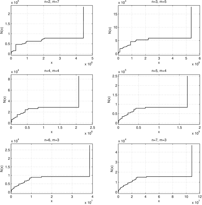
Figure 7. Eigenvalue counting function on $\mathcal{VS}_{n}$ for $n=2,\ldots,7$. Here $m$ refers to the level of the graph approximation.

Since the eigenvalue counting function grows as $x^{\alpha}$ where $\alpha=\log(4n-3)/\log((4n-3)(2n-1))$, it is also useful to look at the Weyl ratio $N(x)/x^{\alpha}$, shown in Figure 8.

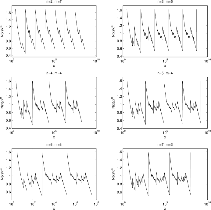
Figure 8. Weyl ratios on $\mathcal{VS}_{n}$ for $n=2,\ldots,7$. Here $m$ refers to the level of the graph approximation.

For each $n$, these functions are asymptotically periodic as a function of $\log x$, as predicted in [17]. What is rather striking and somewhat mysterious, there appears to be a convergence as $n\to\infty$, after appropriate rescaling. We will attempt to explain some of this in Section 11.

We can also compute eigenfunctions of the graph Laplacians. Figure 9 shows 0-series eigenfunctions and their restrictions to the diagonal, and Figure 10 shows the same for some 4/3-series eigenfunctions. The eigenfunctions in the diagonal plots have been continued with the lowest inverse several times to increase the number of data points.

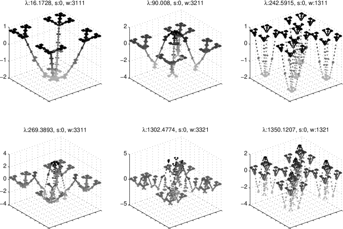
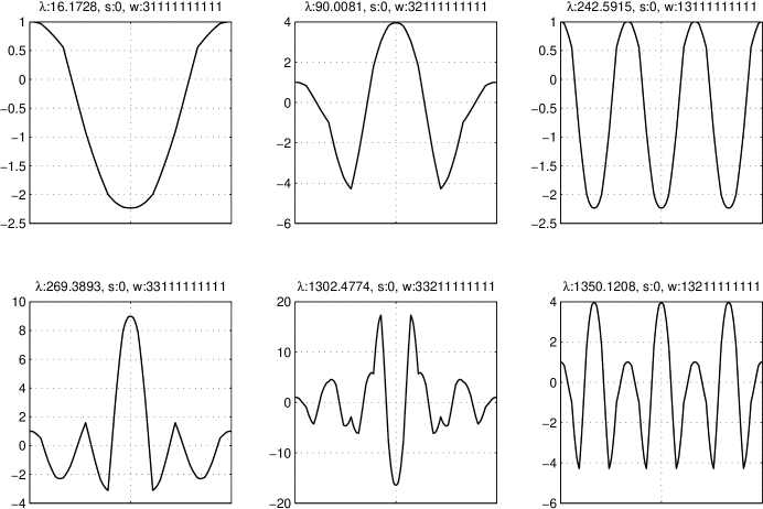
Figure 9. Some 0-series eigenfunctions on $\mathcal{VS}_{2}$ and their restrictions to the diagonal.

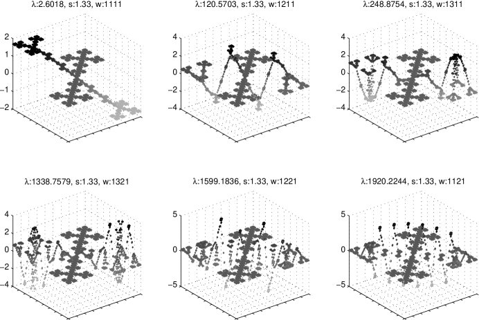
Figure 10. Some 4/3-series eigenfunctions on $\mathcal{VS}_{2}$ and their restrictions to the diagonal.

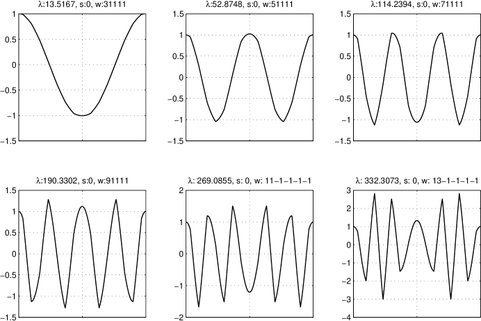
Figure 11. Some 0-series eigenfunctions on $\mathcal{VS}_{8}$, restricted to the diagonal.

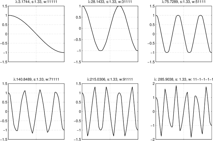
Figure 12. Some 4/3-series eigenfunctions on $\mathcal{VS}_{8}$, restricted to the diagonal.

For $n>2$, our implementation can only compute eigenfunctions restricted to the diagonal. ./figures 11 and 12 show these plots for $\mathcal{VS}_{8}$. There is more data on the website [7].

We observe from the data a phenomenon known as miniaturization [4]. Taking a 0-series eigenfunction on the $m$th level approximation to $\mathcal{VS}_{2}$, if the function is continued by spectral decimation to the $(m+1)$th level of approximation, the new eigenfunction is composed of 5 copies of the previous one; it is “miniaturized.” Thus, eigenfunctions of higher eigenvalue are composed of copies of eigenfunctions of lower eigenvalue.

5. Spectral operators

We can apply the theory of spectral operators to finding solutions of differential equations on the Vicsek set. Two major equations are the heat equation and the wave equation.

5.1. Heat Kernel

The heat equation for a function $u(x,t)$ with Neumann boundary conditions states

$$\left\{\begin{aligned} \frac{\partial u}{\partial t}&=\Delta_{x}u(x,t),\\ \partial_{n}u(q_{j},t)&=0,\\ u(x,0)&=f(x).\end{aligned}\right.$$

Formally this is solved by

$$u(x,t)=e^{t\Delta}f(x)$$

and since the Laplacian has a discrete spectrum with an orthonormal basis $\{u_{j}\}$ of eigenfunctions, $-\Delta u_{j}=\lambda_{j}u_{j}$, the solution to the heat equation is

$$u(x,t)=\sum_{j}e^{-t\lambda_{j}}\left(\int f(y)u_{j}(y)d\mu(y)\right)u_{j}(x).$$

Usually the sum and integral can be interchanged to yield

$$u(x,t)=\int h(t,x,y)f(y)d\mu(y)$$

where $h$ is defined to be

$$h(t,x,y)=\sum_{j}e^{-t\lambda_{j}}u_{j}(x)u_{j}(y)$$

and called the heat kernel.

From the eigenvalues and eigenfunctions we can construct the heat kernel on the standard Vicsek set. This is especially easy when one of the arguments is the center point of the Vicsek set, since then we only need to consider 0-series eigenfunctions. Plots of the heat kernel on the $m=4$ approximating graph are shown in Figure 13.

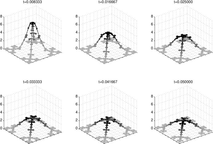
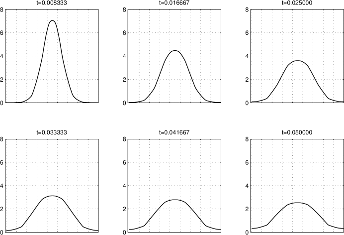
Figure 13. The heat kernel $h(t,q_{0},x)$ on $\mathcal{VS}_{2}$ for various values of $t$, on the whole Vicsek set and restricted to the diagonal

Our data allows us to examine the behavior of the heat kernel $h(t,q_{0},x)$ in greater detail. Estimates for the heat kernel are known, but they involve constants of unknown size. It is expected that $h(t,q_{0},x)$ should involve a factor of $t^{-\alpha}$ multiplying a term that drops off exponentially as $x$ moves away from $q_{0}$. Since that data in Figure 18 suggest that the $t^{-\alpha}$ factor is modified by an oscillating factor, we look at the ratio $h(t,q_{0},x)/h(t,q_{0},q_{0})=H(t,x)$. Actually, it seems more plausible that

$$\frac{h(t,q_{0},x)}{\sqrt{h(t,q_{0},q_{0})}\sqrt{h(t,x,x)}}$$

will be better behaved than $H(t,x)$, but since we don’t know how to compute $h(t,x,x)$ effectively, this isn’t an option. Note that $H(t,x)$ is normalized so that $H(t,q_{0})=1$. Also, if we ignore the influence of the boundary, which is certainly very slight for small $t$, we expect $H(t/15,F_{0}x)$ should be very close to $H(t,x)$. Figure 14

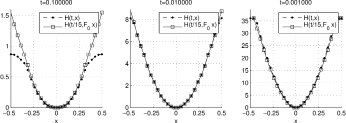
Figure 14. $H(t,x)$ and $H(t/15,F_{0}x)$ on the diagonal (using the $m=4$ graph approximation).

illustrates this invariance property.

First we look at the behavior of $H(t,x)$ for $x$ restricted to the diagonal. Figure 15

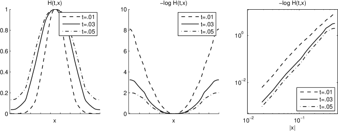
Figure 15. $H(t,x)$ and $-\log H(t,x)$ for several choices of $t$ (using the $m=4$ graph approximation).

shows some typical graphs. We also look at $-\log H(t,x)$, again shown in Figure 15. Since $-\log H(t,x)$ vanishes at $x=q_{0}$, we try to fit a power law $-\log H(t,x)\approx a|x|^{b}$ where the constants $a$ and $b$ depend on $t$, and $|x|$ denotes the distance to $q_{0}$. However, we find that the power $b$ varies significantly as we vary the neighborhood of $q_{0}$ where we do the fit. This leads us to doubt the power law model. Figure 15 shows a log-log plot of $-\log H(t,x)$ for some choices of $t$.

There is no compelling reason to restrict $x$ to the diagonal in studying the heat kernel. In a crude sense, the heat kernel $h(t,q_{0},x)$ should depend on the distance of $x$ to $q_{0}$ in the resistance metric, which coincides with geodesic distance in $\mathcal{VS}_{2}$. But in fact, this is not very accurate. What we want to look at are what might be called “heatballs”, sets of the form

$$\{x:h(t,q_{0},x)\geq s\}$$

for different choices of $t$ and $s$. A naive guess would be that the heatballs form a 1-parameter family of sets, at least if we stay toward the center of $\mathcal{VS}_{2}$ where the influence of the boundary is small. Again this is only valid in a crude sense. Figure 16

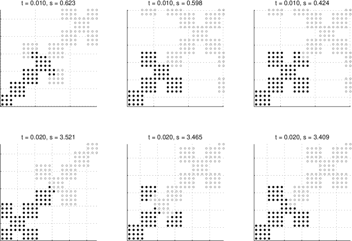
Figure 16. Some heatballs for $t=.01,.02$.

shows some examples of heatballs for two different choices of $t$ and a variety of $s$-values. One observation is that heatballs tend to spread further in directions perpendicular to the diagonal. Decreasing the value of $s$ increases the size of the heatballs, so we may imagine that the heatballs for fixed $t$ represent an “invasion” that spreads out from the center point $q_{0}$. By and large the invasion follows an orderly patter, with a cells that lies on the diagonal being invaded first at the point closest to $q_{0}$. However, there are examples where the invasion jumps around, and this produces examples of heatballs that are disconnected. Apparently, disconnected heatballs also may occur in the setting of manifolds [14]. Of course, it is also possible to study invasions with $s$ fixed and $t$ increasing.

The trace of the heat kernel and its value at the center, when multiplied by $t^{\alpha}$, are both periodic in $\log t$ (see [13]). This is shown in ./figures 17 and 18 on the $m=7$ graph approximation. The approximate sinusoidal behavior is explained for the trace in [2], and at the center in [13]. We note that the approximate sines are out of phase: Fitting to $a+b\sin(c\log t+d)$ we get $a=.90$, $b=.045$, $c=2.33$, and $d=-2.2$ for the trace of the heat kernel, and $a=.4110$, $b=.0191$, $c=2.33$, and $d=1.803$ for the heat kernel at the center.

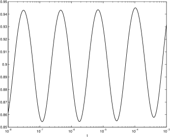
Figure 17. Plot of $t^{\alpha}\int h(t,x,x)\,d\mu(x)$ versus $t$ on the $m=7$ graph approximation to $\mathcal{VS}_{2}$.

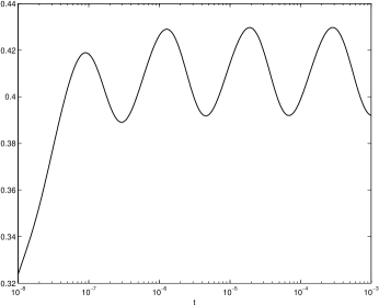
Figure 18. Plot of $t^{\alpha}h(t,q_{0},q_{0})$ versus $t$ on the $m=7$ graph approximation to $\mathcal{VS}_{2}$.

5.2. Wave Propagator

The wave equation is given by

$$\frac{\partial^{2}u}{\partial t^{2}}=\Delta u$$

If we impose Neumann boundary conditions and initial conditions $u(x,0)=0$, $\frac{\partial}{\partial t}u(x,0)=f(x)$, then the solution is given by

$$u(x,t)=\int W(t,x,y)f(y)d\mu(y)$$

where the wave propagator $W(t,x,y)$ is given by

$$W(t,x,y)=\sum\frac{\sin\sqrt{\lambda_{j}}t}{\sqrt{\lambda_{j}}}u_{j}(x)u_{j}(y).$$

From the eigenvalues and eigenfunctions we can also construct the wave propagator on the standard Vicsek set. As with the heat kernel, this is easiest to compute when on of the arguments is the center point of the Vicsek set, since then we only need to consider 0-series eigenfunctions. This is shown in Figure 19.

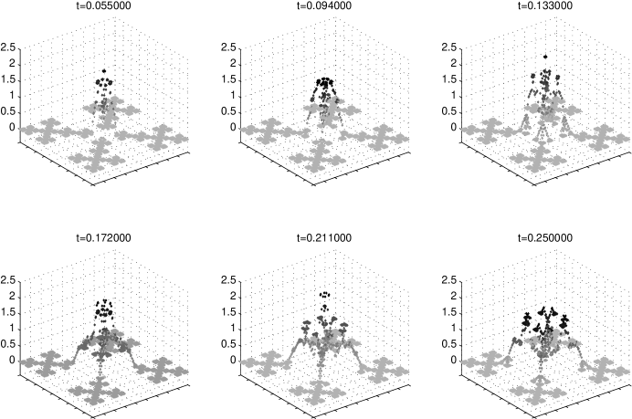
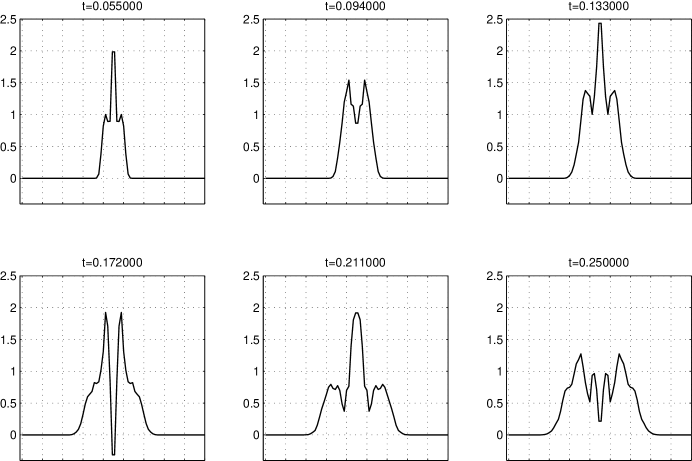
Figure 19. The wave propagator $w(t,q_{0},x)$ on $\mathcal{VS}_{2}$ for various values of $t$, on the whole Vicsek set and restricted to the diagonal.

As already observed in the case of $\mathcal{SG}$ in [8] the wave propagator $W(t,q_{0},x)$ is not supported in a small neighborhood of $q_{0}$ for fixed $t$; in other words, waves propagate at infinite speed. This is easily explained because the differential operators on either side of the wave equation do not have the same order. However, the amount of energy that propagates at high speed is relatively small. So we can expect a weak substitute for finite propagation speed. Attempts to understand this in [8] and [6] were stymied by the complexity of the wave propagator on $\mathcal{SG}$ (in [2] it was shown that time integrals of the wave propagator are computationally tamer on $\mathcal{SG}$, but this did not help with a weak finite propagation speed).

On $\mathcal{VS}_{2}$ the wave propagator at the center point may be effectively computed. In particular, when we increase the level of approximation the graph does not change appreciably: Figure 20 shows $L^{2}$ distances between $w_{m}(t,q_{0},\cdot)$ and $w_{m-1}(t,q_{0},\cdot)$, where $w_{m}$ is the level $m$ approximation to the wave propagator.

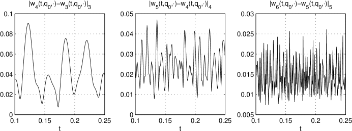
Figure 20. $L^{2}$ distances between $w_{m}(t,q_{0},\cdot)$ and $w_{m-1}(t,q_{0},\cdot)$.

In Figure 19 we display the graphs for some values of $t$. Unlike the heat kernel, the wave propagator is not known to be positive, and indeed we see time where negative values occur. We know

$$\int W(t,q_{0},x)d\mu(x)=t$$

so that positive values predominate, and it seems from the data that

$$\int|W(t,q_{0},x)|d\mu(x)$$

is bounded by a multiple of $t$. Recall that in Euclidean space, the singularity of the wave propagator worsens as the dimension increases. Our data is more in line with the $n=1$ case.

Our data strongly suggests an approximate finite propagation speed. We can quantify this by choosing a small cutoff $\varepsilon$ and looking for the maximum value of $|x|$ where $|w_{m}(t,q_{0},x)|\geq\varepsilon$ for fixed $t$, and then letting $t$ vary. In Figure 21

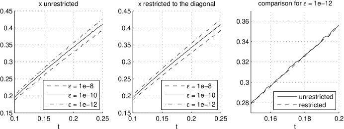
Figure 21. $\max\{|x|:|w_{6}(t,q_{0},x)|\geq\varepsilon\}$ for several choices of $\varepsilon$, both in the case when $x$ is restricted to the diagonal and when $x$ varies over all $\mathcal{VS}_{2}$.

we show plots of this function, both in the case when $x$ is restricted to the diagonal and in the case where $x$ varies over all $\mathcal{VS}_{2}$, for different choices of $\varepsilon$. Notice that in both cases the slope of the function increases with $\varepsilon$.

5.3. Spectral Projections

Another important class of spectral operators are the spectral projections. Let $\Lambda$ be a subset (usually infinite) of the spectrum, and define

$$P_{\Lambda}f=\sum_{\lambda\in\Lambda}P_{\lambda}f$$

where

$$P_{\lambda}f(x)=\sum\int u_{j}(x)u_{j}(y)f(y)d\mu(y)$$

for $\{u_{j}\}$ an orthonormal basis of the $\lambda$-eigenspace. Such operators are always bounded on $L^{2}$ (with norm 1) and usually not bounded on $L^{1}$ or $L^{\infty}$. A natural question to ask is under what conditions is $P_{\Lambda}$ bounded on $L^{p}$ for $1<p<\infty$? In the classical setting such results can be obtained from the Marcinkiewicz multiplier theorem [20] and we expect that analogous results should be valid in the fractal setting, perhaps related to the transplantation theorems of [10] and [19]. We note that the results of [21] imply that we can always “segment” such problems; we write $\Lambda_{k}=\Lambda\cap[0,N_{k}]$ for a natural sequences of cutoffs $N_{k}$ that lie at the beginning of spectral gaps (in our case we take spectral decimation through level $k$). Then $P_{\Lambda}$ is bounded on $L^{p}$ if and only if $P_{\Lambda_{k}}$ is uniformly (in $k$) bounded on $L^{p}$.

In [2] we looked at some spectral projection on $\mathcal{SG}$, but it was difficult to arrive at meaningful predictions because of the computational complexity of the data. Here we are able to examine one example in detail: the case that $\Lambda$ consists of the 0-series eigenvalues. Because these eigenvalues all have multiplicity one, it is straightforward to compute kernels $K_{k}(x,y)$ of the segmented projection operators $P_{\Lambda_{k}}$ for $k\leq 5$ on $\mathcal{VS}_{2}$. We make a few simple observations. The first is that

$$\int K_{k}(x,y)d\mu(y)=1\qquad\text{for every $x$}.$$

This follows from the fact that the constant 1 is in the 0-series, and every other 0-series eigenfunction is orthogonal to it. The second is that

$$K_{k}(x,y)=K_{k}(\Phi(x),y)=K_{k}(x,\Phi(y))=K_{k}(\Phi(x),\Phi(y))$$

where $\Phi$ is any isometry of $\mathcal{VS}_{2}$. This is an immediate consequence of the fact that each 0-series eigenfunction is invariant under $\Phi$ (if $u$ is a 0-series eigenfunction then so is $u\circ\Phi$, with the same eigenvalue, and the multiplicities are all one). Incidentally, we remark that invariance under all isometries does not characterize the 0-series spectrum; it easy to construct 4/3-series eigenfunctions (on a higher level) that show this invariance.

We examine the behavior of $\int|K_{k}(x,y)|d\mu(y)$ as a function $k$. Table 1

$k$	$\max_{x}\textstyle\int|K_{k}(x,y)|d\mu(y)$
1	1.4476
2	1.7336
3	2.9958
4	4.7955
5	7.6572

Table 1. Maximum value of $\int|K_{k}(\cdot,y)|d\mu(y)$ for several $k$.

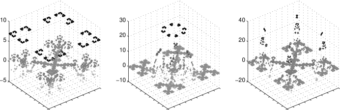
Figure 22. $K_{4}(x,\cdot)$ for $x=q_{1},F_{0233}q_{3},F_{2042}q_{2}$

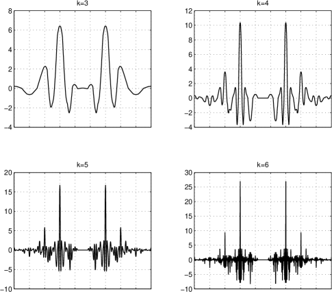
Figure 23. The restriction of $K_{k}(x,\cdot)$ to the diagonal when $x$ is the junction point between two 1-cells, for $3\leq k\leq 6$.

shows the maximum over $x$ for $k\leq 5$. This is overwhelming evidence that $\max_{x}\int|K_{k}(x,y)|d\mu(y)\to\infty$ as $k\to\infty$, and this implies that $P_{\Lambda}$ is not bounded in $L^{1}$ or $L^{\infty}$. Next we ask, for fixed $x$, what are the $y$ values where $|K_{k}(x,y)|$ is large? Looking at the graphs of $K_{k}(x,\cdot)$ in Figure 22 we see evidence that the answer is the values of $y$ that are close to $\Phi(x)$ for some isometry $\Phi$. Note that for some choices of $x$, the set of all $\Phi(x)$ is finite, but for other choices it may be infinite. (For example, if $x$ is a boundary point, then it is a dense subset of a Cantor set that includes the intersection of $\mathcal{VS}_{2}$ with the boundary of the unit square.)

In Figure 23 we show the restriction to the diagonal of $K_{k}(x,\cdot)$ when $x$ is the junction point between two 1-cells, for $3\leq k\leq 6$. The behavior is certainly more complicated than the kernels in the standard Calderon-Zygmund theory. On the other hand, the graphs to appear to be converging to some limiting shape. It would be interesting to make this statement more precise, and to investigate whether there is $L^{p}$ boundedness of $P_{\Lambda}$ for some values of $p$ in $1<p<\infty$ other than $p=2$.

6. Diagonals and the 0-series

We can write $L^{2}(\mathcal{VS})=\mathcal{H}_{0}\oplus\mathcal{H}_{4/3}$ where $\mathcal{H}_{0}$ represents the eigenfunctions associated with the 0-series, and $\mathcal{H}_{4/3}$ represents those associated with the 4/3-series. These are orthogonal because the eigenvalues are distinct.

Theorem 6.1.

Each 0-series eigenfunction of the Laplacian on the Vicsek Set is determined by its restriction to the diagonal.

Proof.

If we look at the fractal Laplacian, we can view $\mathcal{VS}$ as the union of the diagonals with little trees attached, each tree a small copy of $1/4\,\mathcal{VS}$, one arm of the Vicsek set. $u|_{T}$ satisfies $-\Delta u=\lambda u$, with $\partial_{n}u=0$ at the outer boundary, and $u(q_{0})$ is a specified value if $q_{0}$ is the center point, because the center point lies on the diagonal.

Let $v_{\lambda}$ denote the function on $1/4\,\mathcal{VS}$ that satisfies $-\Delta v_{\lambda}=\lambda v_{\lambda}$, $\partial_{n}v_{\lambda}(q)=0$ if $q$ is a boundary point, and $v_{\lambda}(q_{0})=1$. To show existence and uniqueness, we have to show that $-\Delta u=\lambda u$ on $1/4\,\mathcal{VS}$, $\partial_{n}u(\textup{boundary})=0$, and $u(q_{0})=0$ imply that $u$ must be identically zero. Indeed, given such a function $u$, extend it by odd reflection across the center to the opposite arm of the Vicsek set, and set it identically zero on the other two arms. Then we obtain a global eigenfunction satisfying $\sum u(q_{j})=0$ for the boundary points $q_{j}$, so it belongs to the 4/3-series. But $\lambda$ is a 0-series eigenvalue, and by spectral decimation, there are no simultaneous 0-series and 4/3-series eigenvalues; the only way out is if $u=0$.

Now let $T$ denote any tree of level $m$ that attaches to the diagonal at $y$. Then there exists $\psi_{T}:T\to 1/4\,\mathcal{VS}$ with $\psi_{T}(y)=q_{0}$ and $\psi_{T}(\textup{bdry}(T))=\textup{bdry}(1/4\,\mathcal{VS})$, and

$$\Delta(f\circ\psi_{T})=(15)^{m}(\Delta f)\circ\psi_{T}.$$

This says that any tree can be put in one-to-one correspondence with an arm of the Vicsek set in such a way as to respect similarities.

Let $u$ be our 0-series eigenfunction. Then $(u|_{T})\circ\psi_{T}^{-1}=f$ satisfies

$$-\Delta f =(15)^{-m}\lambda f\quad\text{on $1/4\,\mathcal{VS}$,}$$

$$\partial_{n}f(\textup{bdry}) =0,$$

$$f(q_{0}) =u(y).$$

Since $(15)^{-m}\lambda$ is not a 4/3-series eigenvalue (if it were, then so would $\lambda$ be) we have $f=u(y)v_{15^{-m}\lambda}\circ\psi_{T}$. Hence

$$u|_{T}=u(y)v_{15^{-m}\lambda}\circ\psi_{T}.$$

So $\lambda$ and $u|_{\rm diagonal}$ determine $u$ according to the above equation. ∎

We would like to go further and say that any function in $\mathcal{H}_{0}$ is determined by its restriction to the diagonal, and aside from symmetry there are essentially no other conditions on the restrictions to the diagonal of $\mathcal{H}_{0}$ functions. We begin with the analogous statement on the discrete approximations.

Let $D_{m}$ denote the intersection of $V_{m}$ with one arm of the diagonal. Note that $\#D_{0}=1$, $\#D_{1}=2$ and $\#D_{m}=3\#D_{m-1}-1$. Let $Z_{m}$ denote the span of the 0-series eigenfunctions through level $m$. We may consider elements of $Z_{m}$ as functions either on $V_{m}$ or $\mathcal{VS}_{2}$. Note that $\dim Z_{0}=1$, $\dim Z_{1}=2$ and $\dim Z_{m}=3(\dim Z_{m-1})-1$, so $\dim Z_{m}=\#D_{m}=\frac{1}{2}(3^{m}+1)$. Thus it is plausible that every function on $D_{m}$ is the restriction of a function in $Z_{m}$, and every function in $Z_{m}$ is uniquely determined by its restriction to $D_{m}$. In fact, these statements are equivalent. We conjecture a little more.

Let $x_{0},x_{1},x_{2},\ldots$ denote the points in $D_{m}$ moving from the outside inward. Let $D_{m}^{(k)}=\{x_{0},\ldots,x_{k}\}$ and let $V_{m}^{(k)}$ denote all points in $V_{m}$ that attach to one of the midpoints of the intervals in $D_{m}^{(k+1)}$.

Conjecture.

If $f\in Z_{m}$ vanishes on $D_{m}^{(k)}$, then it vanishes on $V_{m}^{(k)}$. In particular, $f$ is determined on $V_{m}$ by its values on $D_{m}$.

This conjecture implies that there is a formula of the form

$$f(z)=\sum c_{k}^{(m)}(z)f(x_{k})$$

for all $f\in Z_{m}$ for each $z\in V_{m}$ and suitable coefficients $c_{k}^{(m)}$. In fact $f(z)=c_{k}^{(m)}(z)$ defines the function in $Z_{m}$ that takes on the values $f(x_{j})=\delta_{jk}$ on $D_{m}$. The conjecture implies $c_{k}^{(m)}(z)=0$ if $z\in D_{m}^{(k)}$.

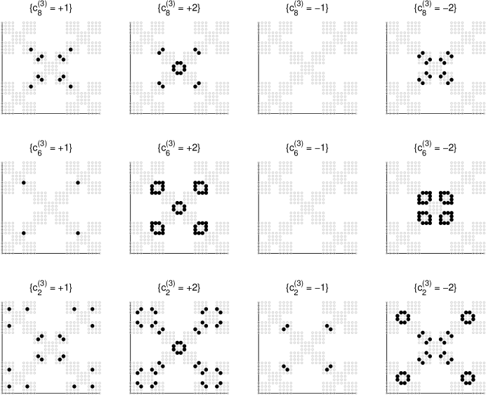
Figure 24. The values of $c_{k}^{(3)}$ for three choices of $k$.

Experimental evidence indicates that $c_{k}^{(m)}$ can take on only 4 nonzero values, namely $\pm 1$ and $\pm 2$. Some examples of $c_{k}^{(3)}$ are shown in Figure 24 and many more are available (for $m=4$) on our website [7].

To pass from the discrete to the continuous version we consider function $\mathcal{H}_{0}\cap C$ (here $C$ denotes the continuous functions on $\mathcal{VS}_{2}$). Such functions have well-defined restrictions to $D$ (one arm of the diagonal). To show that the restriction $f|_{D}$ of such a function determines $f$, it suffices to show that it determines $f|_{V_{m}}$ for all $m$, since $\cup_{m}V_{m}$ is dense in $\mathcal{VS}_{2}$ and $f$ is continuous. Let $f_{m}$ denote the projection of $f$ onto $Z_{m}$. By the results of [21] we know $f_{m}$ converges to $f$ uniformly. If the conjecture is valid then $f_{m^{\prime}}(z)=\sum c_{k}^{(m)}f_{m^{\prime}}(x_{k})$ for $z\in V_{m}$ and $m^{\prime}\geq m$ (since $f_{m^{\prime}}|_{V_{m}}\in Z_{m}$), so passing to the limit $f(z)=\sum c_{k}^{(m)}f(x_{k})$ for $z\in V_{m}$. Despite the fact that this is a finite sum for each $m$, it is a rather peculiar formula. The coefficients oscillate rapidly but do not go to zero as $m$ increases. It does not seem likely that we can make any sense out of it if we do not assume that $f$ is continuous. It seems unlikely that the existence of a continuous restriction to $D$ for a function in $\mathcal{H}_{0}$ implies that it is continuous on $\mathcal{VS}_{2}$. A more plausible conjecture is that if the restriction to $D$ is Hölder continuous of some order then the function is Hölder continuous of the same order on $\mathcal{VS}_{2}$. Another reasonable conjecture is that the restrictions of $\mathcal{H}_{0}\cap C$ to $D$ form a dense subset of the continuous functions on $D$. A less likely conjecture is that the restrictions give all continuous functions on $D$.

7. Ratio Gaps

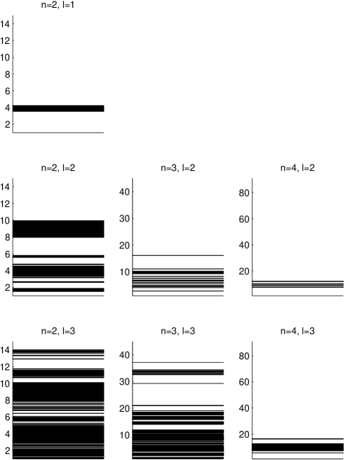
Figure 25. Ratio gaps for $n=2,3,4$ and $\ell=|w|=1,2,3$. The gaps are the black regions. No gaps were found for $n=3,4$ and $\ell=1$.

In [5] it was shown that on $\mathcal{SG}$ there exist gaps in the ratios of eigenvalues. As a consequence, it is possible to define operators of the form $\Delta^{\prime}-a\Delta^{\prime\prime}$ on the product of two copies of $\mathcal{SG}$ ($\Delta^{\prime}$ and $\Delta^{\prime\prime}$ denote the Laplacian on each copy of $\mathcal{SG}$) where $a$ lies in a gap, and these operators paradoxically behave in some ways like elliptic operators, despite the fact that the coefficient $-a$ has the wrong sign. These operators were called quasielliptic in [5]. There are no analogous operators in classical PDE theory. Thus it is of great interest to know whether similar operators exist for products of fractals other than $\mathcal{SG}$. In fact [15] shows that this is the case for $\mathcal{VS}_{2}$ and $\mathcal{VS}_{3}$. Also [9] investigates this question for a variant of the $\mathcal{SG}$ type fractal. The method used in [9], which we follow here, yields a computer-assisted proof. The idea is that the method introduced in [5] leads to a large number of tedious calculations, and these are best left to the computer. In our method there is a parameter $\ell$ that may be chosen at will. Increasing $\ell$ will do a better job finding gaps, at the cost of increasing the number of computations.

Let $\lambda_{m}$ be a graph eigenvalue born on level $m_{0}$. Then

$$\lambda_{m}=\phi_{w_{m}}\circ\phi_{w_{m-1}}\circ\cdots\circ\phi_{w_{m_{0}+1}}(\lambda_{m_{0}})$$

where $\lambda_{m_{0}}\in\{0,4/3\}$. Let $p$ be the fixed point of $\phi_{2n-1}$ and $q=\phi_{2n-1}(4/3)$. If $\lambda_{m_{0}}=0$ we have $\lambda_{m}\leq p$, while if $\lambda_{m_{0}}=4/3$ then we either have $m=m_{0}$ and $\lambda_{m}=4/3$ or $\lambda_{m}\leq q$. Since $q\geq p$, we can simply write

(7.1) $$\lambda_{m}\in[0,q]\cup\{4/3\}.$$

Fix $\ell>0$. Any fractal eigenvalue $\lambda$ is of the form

$$\lambda =\rho^{m_{0}}\lim_{m\to\infty}\rho^{m}\phi_{v_{m}}\circ\phi_{v_{m-1}}\circ\cdots\circ\phi_{v_{m_{0}+1}}(\lambda_{m_{0}})$$

where all but finitely many of the $v_{j}=1$. Thus there must be a word $w$ of length $\ell$ and some graph eigenvalue $\lambda_{m}$ so that

$$\lambda =\rho^{m_{0}}\lim_{k\to\infty}\rho^{k}\phi_{1}^{k}\circ\phi_{w}\circ\phi_{v_{m}}\circ\cdots\circ\phi_{v_{m_{0}+1}}(\lambda_{m_{0}})$$

$$=\rho^{m_{0}+\ell+m}\lim_{k\to\infty}\rho^{k}\phi_{1}^{k}(\phi_{w}(\lambda_{m}))$$

$$=\rho^{m_{0}+\ell+m}\psi_{n}(\phi_{w}(\lambda_{m})),$$

($\phi_{w}=\phi_{w_{\ell}}\circ\cdots\circ\phi_{w_{1}}$). Combining this with (7.1) we see that every fractal eigenvalue $\lambda$ can be written as

(7.2) $$\lambda=\rho^{r}\psi_{n}(x),\qquad x\in\bigcup_{|w|=\ell}\phi_{w}([0,q]\cup\{4/3\}).$$

for some integer $r$.

Consider the contribution of a word $w$ to the eigenvalues described by (7.2). If $w$ ends in a $1$, then as long as $m>m_{0}$ can rewrite

$$\phi_{w}\circ\phi_{v_{m}}\circ\cdots\circ\phi_{v_{m_{0}+1}}(\lambda_{m_{0}})=\phi_{1}\circ\phi_{w^{\prime}}\circ\phi_{v_{m-1}}\circ\cdots\circ\phi_{v_{m_{0}+1}}(\lambda_{m_{0}}),$$

for some other word $w^{\prime}$ of length $\ell$ (with one less 1 at the end), while $m=m_{0}$ means

$$\phi_{w}\circ\phi_{v_{m}}\circ\cdots\circ\phi_{v_{m_{0}+1}}(\lambda_{m_{0}})=\phi_{w}(\lambda_{m_{0}})\in\left\{\phi_{w}(0),\phi_{w}(4/3)\right\}.$$

Thus (7.2) is still valid with $\phi_{w}([0,q]\cup\{4/3\})$ replaced by $\{\phi_{w}(0),\phi_{w}(4/3)\}$ in (7.2) for every word $w$ ending in 1. Furthermore we can discard $\phi_{w}(\lambda_{m_{0}})$ if it is forbidden.

So far we’ve found finitely many intervals $[a_{i},b_{i}]$ (allowing $a_{i}=b_{i}$) so that each eigenvalue $\lambda$ must satisfy

$$\lambda\in\rho^{r}\psi_{n}([a_{i},b_{i}])=\rho^{r}[\psi_{n}(a_{i}),\psi_{n}(b_{i})]$$

for some $i$ and $r$. Therefore any ratio of eigenvalues $\lambda/\mu$ must satisfy

$$\frac{\lambda}{\mu}\in\rho^{r}\left[\frac{\psi_{n}(a_{i})}{\psi_{n}(b_{j})},\frac{\psi_{n}(b_{i})}{\psi_{n}(a_{j})}\right]\equiv\rho^{r}[R_{ij},S_{ij}]$$

for some $r$, $i$, and $j$. Since $\rho\lambda$ is an eigenvalue if $\lambda$ is, we can restrict our attention to ratios $\lambda/\mu\in[1,\rho]$ and hence to the finite number of intervals $\rho^{r}[R_{ij},S_{ij}]$ which intersect $[1,\rho]$. The gaps in the union of these intervals are then guaranteed to be ratio gaps.

Figure 25 shows the ratio gaps that are proved to exist by this method for $n=2,3,4$ using values of $\ell=1,2,3$. For all of these $n$ there are ratio gaps containing $\sqrt{\rho_{n}}$, given in Table 2.

$n$	$\sqrt{\rho_{n}}$	$\ell$	ratio gap
2	3.8730	1	$[3.5370,4.2409]$
		2	$[3.2948,4.5526]$
		3	$[3.2948,4.5526]$
3	6.7082	1	no gap
		2	$[6.6952,6.7212]$
		3	$[6.6950,6.7214]$
4	9.5394	1	no gap
		2	no gap
		3	$[9.5357,9.5431]$

Table 2. Ratio gaps containing $\sqrt{\rho_{n}}$ for $n=2,3,4$ and $\ell=1,2,3$.

We see clearly that the number and size of the ratio gaps increases with $\ell$. However, we have not been able to confirm the existence of ratio gaps for $n\geq 5$. For $n=5$ none are revealed for $\ell\leq 2$ and our MATLAB implementation (see [7]) runs into memory problems for $\ell\geq 3$. For $\ell\geq 3$ we can, however, use a modified algorithm which searches only for ratio gaps containing a particular point. These searches have failed to find ratio gaps containing $\sqrt{\rho_{5}}\approx 12.3693$. It is not clear if these failed searches should be interpreted as experimental evidence for the nonexistence of ratio gaps, or just as evidence that we need to consider higher values of $\ell$ to find ratio gaps.

8. Eigenvalue clusters

We say the spectrum of a Laplacian exhibits spectral clustering if the following holds: for every integer $n$ and $\varepsilon>0$ there exists an interval $I$ of length $\varepsilon$ that contains $n$ distinct eigenvalues.

This, for example, says you can find a million distinct eigenvalues within a millionth of each other. The eigenvalues will have to be very large, so it becomes computationally challenging to find such tight and large clusters. Clustering does not occur on the Sierpinski gasket $\mathcal{SG}$. Experimental evidence suggests that it does occur on the pentagasket [1] and on the Julia sets [11]. The following lemma allows us to prove it holds on $\mathcal{VS}_{2}$.

Lemma 8.1.

Suppose spectral decimation holds with spectral renormalization factor $\rho$ and spectral renormalization function $R(\lambda)$. Suppose $R$ has a fixed point $t$ ($R(t)=t$) such that $|R^{\prime}(t)|>\rho.$ Then spectral clustering occurs.

Proof.

Let $\phi_{1},\phi_{2},\ldots\phi_{N}$ be the inverses of $R(\lambda)$ in increasing order. Then $\phi_{1}(0)=0$ and $\phi_{1}^{\prime}(0)=1/\rho$. There exists $k$ such that $\phi_{k}(t)=t$ and $|\phi_{k}^{\prime}(t)|=b<\rho^{-1}$, by the assumption. Choose $m$ large enough that $\Delta_{m}$ has at least $n$ distinct eigenvalues $\lambda_{1},\ldots,\lambda_{n}$. Then $\Delta_{m+j}$ has $n$ distinct eigenvalues $\phi_{k}^{(j)}(\lambda_{1}),\ldots,\phi_{k}^{(j)}(\lambda_{m})$ and these give rise to $n$ distinct eigenvalues

$$\lim_{l\to\infty}\rho^{m+j+l}\phi_{1}^{(l)}\phi_{k}^{(j)}(\lambda_{p}),\qquad 1\leq p\leq n.$$

Write $g(\lambda)=\lim_{l\to\infty}\rho^{l}\phi_{1}^{(l)}(\lambda)$. Then $g$ is a fixed function with bounded derivative $|g^{\prime}(x)|\leq M$ in the relevant interval of length $\varepsilon$ where we want to find $n$ distinct eigenvalues.

By taking $j_{0}$ large enough, we can make all the values $\phi_{k}^{(j_{0})}(\lambda_{p})$ close enough to $t$ so that $|\phi_{k}^{\prime}(x)|\leq a\leq\rho^{-1}$ for all $\phi_{k}^{j_{0}}(\lambda_{p})$. This means that $\{\phi_{k}^{(j_{0}+j_{1})}(\lambda_{p})\}$ belongs to an interval of length no more than $ca^{j_{i}}$ where $c$ is the length for $j_{1}=0$. Then

$$\{\rho^{m+j_{0}+j_{1}}g(\phi_{k}^{j_{0}+j_{1}}(\lambda_{p}))\}$$

belongs to an interval of length at most $cM\rho^{m+j_{0}}(a\rho)^{j_{1}}$. Since $a\rho<1$, this can be made $\leq\varepsilon$ by taking $j_{1}$ large enough. Thus we can find $n$ distinct eigenvalues in an interval of length no more than $\varepsilon$. ∎

On $\mathcal{VS}_{2}$, $\rho=15$ and $R(\lambda)=36\lambda^{3}-48\lambda^{2}+15\lambda$. So $R(t)=t$ means $2t(18t^{2}-24t+7)=0$ with solutions $0,\frac{4\pm\sqrt{3}}{6}$. We are interested in the largest $t$, $\frac{4+\sqrt{2}}{6}$ which is the fixed point of $\phi_{3}$.

$$R^{\prime}(\lambda)=3\cdot 36\lambda^{2}-2\cdot 48\lambda+15=15+12\lambda(9\lambda-8)$$

so to show $R^{\prime}(t)>15$ we need $t>8/9$. But $(4+\sqrt{2})/6=0.902...$ so this is true. We thus have clustering in $\mathcal{VS}_{2}$. Computing the largest fixed point $t$ of $R$ on $\mathcal{VS}_{n}$ for $n=3,\ldots,9$ we also get $R^{\prime}(t)>\rho$ (see Table 3) and hence that spectral clustering occurs. Because the ratio $R^{\prime}(t)/\rho$ increases rapidly with $n$ we conjecture that spectral clustering occurs for all $n$.

$n$	$t$	$\rho$	$R^{\prime}(t)$
2	0.9024	15	1.	$6314\times 10^{1}$
3	0.8905	45	1.	$3999\times 10^{2}$
4	0.8891	91	1.	$2355\times 10^{3}$
5	0.8889	153	1.	$1079\times 10^{4}$
6	0.8889	231	9.	$9655\times 10^{4}$
7	0.8889	325	8.	$9682\times 10^{5}$
8	0.8889	435	8.	$0713\times 10^{6}$
9	0.8889	561	7.	$2641\times 10^{7}$

Table 3. The largest fixed point $t$ of the spectral decimation function $R$ on $\mathcal{VS}_{n}$ satisfies $R^{\prime}(t)>\rho$ for $n=2,\ldots,9$.

9. Green’s Function on $\mathcal{VS}_{n}$

The Green’s function $G$ for the Laplacian is a function satisfying

$$\left\{\begin{aligned} -\Delta G(x,y)&=\delta(x,y)\\ G(q_{j},y)&=0\quad\text{if $q_{j}\in\mathop{\rm bdry}\mathcal{VS}_{n}$}.\end{aligned}\right.$$

where $\delta$ is the Dirac delta function. Then $u(x)=\int G(x,y)f(y)d\mu(y)$ solves

$$\left\{\begin{aligned} -\Delta u&=f,\\ u|_{\mathrm{bdry}}&=0.\end{aligned}\right.$$

As a function of $x$, $G$ should be harmonic in the complement of $y$. Suppose $y$ lies in the upper right arm of $\mathcal{VS}_{n}$. The boundary points are labeled $q_{1},q_{2},q_{3},q_{4}$, with $q_{1}$ corresponding to the arm where $y$ is. Let $z$ be the projection of $y$ onto the diagonal of $\mathcal{VS}_{n}.$ (In the case that $y$ is on the diagonal already, $z=y$.)

Now $G(q_{j},y)=0$ for $j=1,2,3,4$. Define $G(q_{0},y)=a$, (where $q_{0}$ is the center point), $G(z,y)=b$, $G(y,y)=c$. The values $a,b,c$ determine $G$ because $G(x,y)$ is linear on the arms $(q_{0},q_{2}),(q_{0},q_{3}),(q_{0},q_{4})$, on $(q_{0},z)$ and $(z,q_{1})$, and along the unique path joining $z$ to $y$. It is constant on every component of the complement of these 6 sets.

To determine the constants $a,b,c$ we have 3 equations that express $-\Delta_{x}G(q_{0},y)=0$, $-\Delta_{x}G(z,y)=0$, and $-\Delta_{x}G(y,y)=\delta_{y}$. The first two equations say the sum of the 4 derivatives at $q_{0}$ (resp. $z$) vanish. The last says the derivative at $y$ is 1.

For simplicity assume the length of each arm is 1. (This involves rescaling by a factor of $\sqrt{2}/2$ for a unit square.) Let $d(z,q_{0})=s$ (so $d(z,q_{1})=1-s$) and $d(x,y)=t$, measured along the path. Then

$$3a+\frac{a-b}{s} =0\qquad\text{(at $q_{0}$)}$$

$$\frac{b-a}{s}+\frac{b}{1-s}+\frac{b-c}{t} =0\qquad\text{(at $z$)}$$

$$\frac{a-b}{t} =1\qquad\text{(at $y$)}$$

Note that the third equations says $c=b+t$ and the second equation says

$$\frac{b-a}{s}+\frac{b}{1-s}=1.$$

(If $z=y$ then $t=0$, $c=b$, and the second equation says $-\Delta_{x}G(y,y)=1$ as required.) Solving two equations for two unknowns yields

$$a=\frac{1-s}{4},\qquad b=\frac{(1-s)(3s+1)}{4}.$$

In other words,

$$G(q_{0},y) =\frac{1-d(z,q_{0})}{4},$$

$$G(z,y) =\frac{(1-d(z,q_{0}))(3d(z,q_{0})+1)}{4},$$

$$G(y,y) =\frac{(1-d(z,q_{0}))(3d(z,q_{0})+1)}{4}+d(z,y).$$

Denote by $d^{\prime}(x,q_{0})$ the distance from $q_{0}$ to the point on one of the main diagonals where $x$ attaches. So $d^{\prime}(y,q_{0})=d(z,q_{0})$, for example. Then

$$G(x,y)=\frac{(1-d^{\prime}(x,q_{0}))(1-d^{\prime}(y,q_{0}))}{4}$$

if $x$ and $y$ lie on different arms. If $x$ and $y$ lie on the same arm and $d^{\prime}(x,q_{0})<d^{\prime}(y,q_{0})$ then

$$G(x,y)=\frac{(1-d^{\prime}(y,q_{0}))(3d^{\prime}(x,q_{0})+1)}{4},$$

while if $d^{\prime}(y,q_{0})<d^{\prime}(x,q_{0})$ then

$$G(x,y)=\frac{(1-d^{\prime}(x,q_{0}))(3d^{\prime}(y,q_{0})+1)}{4}.$$

If $d(y,q_{0})=d(x,q_{0})$ then

$$G(x,y)=\frac{(1-d^{\prime}(y,q_{0}))(3d^{\prime}(y,q_{0}+1))}{4}+d(z,w(x,y)),$$

where $w(x,y)$ is the last point on the intersection of the paths from $z$ to $y$ and $z$ to $x.$

10. Higher Vicsek Sets

It is clear that $\mathcal{VS}_{n}$ converges to a cross. The eigenfunctions of the Laplacian on the cross are well understood: the restriction to either diagonal is an eigenfunction on the unit interval, while at the center point the function is required to be continuous and to have the sum of its normal derivatives equal to zero. Thus any eigenfunction is either $\cos\pi kx$ on each diagonal or $a_{j}\sin\pi(k+1/2)x$ on each half diagonal, with $\sum a_{j}=0$, for some integer $k$. We call the first type symmetric, and the second nonsymmetric. The symmetric eigenvalues (obtained by taking second derivatives) are $\pi^{2}k^{2}$, and the nonsymmetric eigenvalues are $\pi^{2}(k+1/2)^{2}$.

We claim that the symmetric spectrum is the limit of the spectrum of the 0-series on $\mathcal{VS}_{n}$ as $n\to\infty$ (these are symmetric eigenfunctions), and the nonsymmetric spectrum is the limit of the spectrum of the 4/3-series born on level 0. (the 4/3 series born on levels $\geq 1$ does not contribute to the limit because the eigenvalues go to infinity.) We also claim that the limits of the symmetric eigenfunctions are cosines, and the limits of the nonsymmetric eigenfunctions are sines.

To understand the behavior of the eigenvalues as $n\to\infty$ we can restrict attention to the initial segment consisting of the 0-series eigenvalues $\rho_{n}\psi_{n}(\phi_{2j-1}(0))$ and the 4/3-series eigenvalues $\rho_{n}\psi_{n}(\phi_{2j-1}(4/3))$. From [24] we know

$$r(\lambda)=\lambda g_{n}(\lambda)h_{n}(\lambda),\qquad\text{and}\qquad 3r(\lambda)-4=f_{n}(\lambda)l_{n}(\lambda),$$

so $\phi_{k}(0)$ are the zeroes of $g_{n}$ and $h_{n}$ and $\phi_{k}(4/3)$ are the zeroes of $f_{n}$ and $l_{n}$. The zeroes of $g_{n}$ and $f_{n}$ are forbidden eigenvalues, and correspond to even values of $k$. Thus $\phi_{3}(0),\phi_{5}(0),\ldots,\phi_{2n-1}(0)$ are the zeroes of $h_{n}$ ($\phi_{1}(0)=0$, of course), and $\phi_{1}(4/3),\phi_{3}(4/3),\ldots,\phi_{2n-3}(4/3)$ are the zeroes of $l_{n}$. The exact values

$$\phi_{2j-1}(4/3)=\frac{1+\cos\frac{2\pi(n-j)}{2n-1}}{3}=\frac{2\sin^{2}\frac{\pi}{2}(\frac{2j-1}{2n-1})}{3}$$

are computed in [24]. If $j$ is small compared to $n$, which will always happen if we fix $j$ and let $n\to\infty$, then $\phi_{2j-1}(4/3)\approx\pi^{2}/6(\frac{2j-1}{2n-1})^{2}$. Since $\psi_{n}(t)\sim t$ for $t$ near 0 we have

$$\rho_{n}\psi_{n}(\phi_{2j-1}(4/3))\sim\frac{4n-3}{2n-1}\frac{\pi^{2}}{6}(2j-1)^{2}\to\frac{4\pi^{2}}{3}(j-1/2)^{2}$$

as $n\to\infty$.

There is no exact computation of the zeroes of $h_{n}$, but the zeroes of $g_{n}$ are known, so

$$\phi_{2j}(0)=\frac{1+\cos(\frac{2n-1-2j}{2n-1})\pi}{3}=\frac{2\sin^{2}\frac{\pi}{2}(\frac{2j}{2n-1})}{3}$$

and we have interlacing of zeroes of $g_{n}$ and $h_{n}$, so

$$\phi_{2j-2}(0)<\phi_{2j-1}(0)<\phi_{2j}(0).$$

This implies

$$\frac{4n-3}{2n-1}\frac{\pi^{2}}{6}(2j-2)^{2}\leq\rho_{n}\psi_{n}(\phi_{2j-1}(0))\leq\frac{4n-3}{2n-1}\frac{\pi^{2}}{6}(2j)^{2}.$$

If we assume that the lower bound is the asymptotically correct value, then we obtain the expected value $\frac{4\pi^{2}}{3}(j-1)^{2}$ for the limit. We will show below that this is indeed correct.

We can also understand why the $\mathcal{VS}_{n}$ eigenfunctions, restricted to the cross, converge to the eigenfunctions of the cross. To see this, we look at the graph eigenvalue equation on $V_{1}$. Note that $V_{1}$ consists of four arms of $n-1$ squares joined at a central square. We label the diagonal vertices of one arm $x_{1},x_{2},\ldots,x_{n}$ and the below and above diagonal vertices $y_{1},\ldots,y_{n-1}$ and $z_{1},\ldots,z_{n-1}$ (see Figure 26).

Figure 26. Vertices on one arm of $V_{1}$.

By symmetry we will have $u(y_{j})=u(z_{j})$ for every eigenfunction. The eigenvalue equation (with eigenvalue $\lambda_{1}$) at $y_{j}$ says

$$(1-\lambda_{1})u(y_{j})=\tfrac{1}{3}(u(x_{j})+u(x_{j+1})+u(y_{j}))$$

So we obtain

$$u(z_{j})=u(y_{j})=\frac{u(x_{j})+u(x_{j+1})}{2-3\lambda_{1}}.$$

For $2\leq j\leq n-1$ the eigenvalue equation at $x_{j}$ is

$$(1-\lambda_{1})u(x_{j}) =\frac{1}{6}\Big{(}u(x_{j-1})+u(x_{j+1})+2u(y_{j})+2u(y_{j+1})\Big{)}$$

$$=\frac{1}{6}\left(u(x_{j-1})+u(x_{j+1})+\frac{2u(x_{j-1})+4u(x_{j})+2u(x_{j+1})}{2-3\lambda_{1}}\right).$$

We can simplify this equation to

$$(1-3\lambda_{1})u(x_{j})=\tfrac{1}{2}(u(x_{j-1})+u(x_{j+1})).$$

Note that this is exactly the eigenvalue equation (for eigenvalue $3\lambda_{1}$) on the interior of the linear graph $x_{1},\ldots,x_{n}$. Similarly, at the endpoint $x_{n}$ the eigenvalue equation is

$$(1-\lambda_{1})u(x_{n}) =\frac{1}{3}\Big{(}u(x_{n-1})+2u(y_{n-1})\Big{)}$$

$$=\frac{1}{3}\left(u(x_{n-1})+\frac{2u(x_{n-1})+2u(x_{n})}{2-3\lambda_{1}}\right),$$

which simplifies to

$$(1-3\lambda_{1})u(x_{n})=u(x_{n-1}),$$

and this is the correct eigenvalue equation (for eigenvalue $3\lambda_{1}$) with Neumann conditions at that endpoint.

The equation at the endpoint $x_{1}$ will depend on whether we are looking at the 0-series or the 4/3-series. For the 0-series the values along all four arms will be identical, so the eigenvalue equation is

$$(1-\lambda_{1})(u(x_{1})) =\frac{1}{6}\Big{(}3u(x_{1})+u(x_{2})+2u(y_{1})\Big{)}$$

$$=\frac{1}{6}\left(3u(x_{1})+u(x_{2})+\frac{2u(x_{1})+2u(x_{2})}{2-3\lambda_{1}}\right),$$

which simplifies to

$$\left(1-18\frac{1-\lambda_{1}}{4-3\lambda_{1}}\lambda_{1}\right)u(x_{1})=u(x_{2}).$$

For the 4/3-series the sum of the values on all four arms will be zero, so the eigenvalue equation is

$$(1-\lambda_{1})u(x_{1}) =\frac{1}{6}\Big{(}-u(x_{1})+u(x_{2})+2u(y_{1})\Big{)}$$

$$=\frac{1}{6}\left(-u(x_{1})+u(x_{2})+\frac{2u(x_{1})+2u(x_{2})}{2-3\lambda_{1}}\right),$$

which simplifies to

$$(3-6\lambda_{1})u(x_{1})=u(x_{2}).$$

These should be compared with the eigenvalue equation for the eigenfunction $\tilde{u}$ with eigenvalue $3\lambda_{1}$ on two copies of the linear graph with even and odd symmetries, namely

$$(1-3\widetilde{\lambda}_{1})\tilde{u}(x_{1})=\tfrac{1}{2}(\tilde{u}(x_{2})\pm\tilde{u}(x_{1})).$$

Note that we get the identical equation in the odd case, but in the even case we get

$$(1-6\widetilde{\lambda}_{1})\tilde{u}(x_{1})=\tilde{u}(x_{2}),$$

so there is a significant distinction. In the case of the 4/3-series, we can therefore identify the restriction of the eigenfunctions to the diagonal with

$$\tilde{u}(x_{k})=\sin\pi(j-1/2)\left(\frac{2k-1}{2n-1}\right),\qquad 1\leq j\leq n-1.$$

Figure 27 shows some 0-series eigenfunctions plotted against the symmetric eigenfunctions on the cross for $n=3,6,9$. It appears that $u$ closely approximates

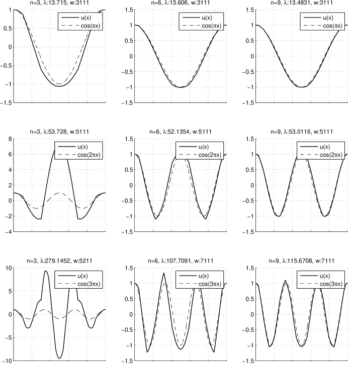
Figure 27. 0-series eigenfunctions on $\mathcal{VS}_{n}$ for $n=3,6,9$ plotted against the corresponding symmetric eigenfunctions on the cross.

$$\tilde{u}(x_{k})=\cos\pi j\left(\frac{2k-1}{2n-1}\right).$$

We now sketch a proof that the eigenvalues $3\lambda_{1}$ approach

$$3\widetilde{\lambda}_{1}=1-\cos\frac{2\pi j}{2n-1}=2\sin^{2}\frac{\pi j}{2n-1}$$

and the eigenvectors $u(x_{k})$ approach $\tilde{u}(x_{k})$ as $n\to\infty$. Here we fix the value of $j$, and we require the appropriate error estimate since both $3\lambda_{1}$ and $3\widetilde{\lambda}_{1}$ tend to zero. The idea is to use standard perturbation theory, using the fact that the two eigenvalue equations differ only at the single point $x_{1}$, and the fact that the eigenvector $\tilde{u}(x_{k})$ is fairly uniformly distributed, so the value $\tilde{u}(x_{1})$ is relatively small.

Let $E$ denote the symmetric $n\times n$ matrix of tridiagonal form, with

$$E_{kk}=\begin{cases}1&2\leq k\leq n-1\\ \frac{1}{2}&k=1\text{~{}or~{}}n\end{cases}$$

and $E_{k(k+1)}=E_{k(k-1)}=-1/2$. Let $\widetilde{G}$ denote the diagonal matrix with

$$\widetilde{G}_{kk}=\begin{cases}1&1\leq k\leq n-1\\ \frac{1}{2}&k=n\end{cases}$$

and let $G$ denote the diagonal matrix with

$$G_{kk}=\begin{cases}1&2\leq k\leq n-1\\ \frac{1}{2}&k=n\\ \frac{3\lambda_{1}-3}{3\lambda_{1}-4}&k=1.\end{cases}$$

Then the two eigenvalue equations may be written

$$Eu =3\lambda_{1}Gu,$$

$$E\tilde{u} =3\widetilde{\lambda}_{1}\widetilde{G}\tilde{u}.$$

Note that the first equation is not a linear generalized eigenvalue equation because $G$ depends on $\lambda_{1}$, but this does not really matter in our argument.

The gist of the argument is that $\widetilde{G}-G$ is a matrix with only one non-zero entry ($\widetilde{G}_{11}-G_{11}$) and we can bound this entry since $\lambda_{1}$ is bounded away from $4/3$ for the 0-series; and also we know $\tilde{u}$ exactly, hence $|\tilde{u}(x_{1})|\leq 1$ while $\langle\widetilde{G}\tilde{u},\tilde{u}\rangle=n/2$. This yields the estimate

$$\frac{\langle(\widetilde{G}-G)\tilde{u},\tilde{u}\rangle}{\langle\widetilde{G}\tilde{u},\tilde{u}\rangle}=O\left(\frac{1}{n}\right).$$

With a little more work, we can get the estimate

$$\frac{\langle(\widetilde{G}-G)\tilde{u},u\rangle}{\langle\widetilde{G}\tilde{u},u\rangle}=O\left(\frac{1}{n}\right)$$

for the first $N$ eigenfunctions ($N$ is fixed as $n\to\infty$). But this is exactly what we need to estimate $\lambda_{1}-\widetilde{\lambda}_{1}$. If we take the inner product of the first eigenvalue equation with $\tilde{u}$ and the second eigenvalue equation with $u$, then using the symmetry of all the matrices we obtain

$$\lambda_{1}\langle G\tilde{u},u\rangle=\widetilde{\lambda}_{1}\langle\widetilde{G}\tilde{u},u\rangle$$

hence

$$\lambda_{1}-\widetilde{\lambda}_{1}=\lambda_{1}\frac{\langle(\widetilde{G}-G)\tilde{u},u\rangle}{\langle\widetilde{G}\tilde{u},u\rangle}=O\left(\frac{1}{n^{3}}\right)$$

for the first $N$ eigenvalues, since we know $\widetilde{\lambda}_{1}=O(1/n^{2})$. With a little more work we can show that $u-\tilde{u}=O(1/n)$ when $u$ is properly normalized.

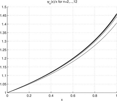
Figure 28. $\psi_{n}(x)/x$ on $[0,1]$ for $n=2,\ldots,12$ ($\psi_{n+1}\geq\psi_{n}$).

So far we have dealt with the level 1 eigenvalues $\lambda_{1}$. The actual eigenvalues $\lambda$ on $\mathcal{VS}_{n}$ are given by $\lambda=\psi_{n}(\lambda_{1})$ for the lowest segment of the spectrum (this will include the first $N$ eigenvalues once $n$ is large enough). Figure 28 gives experimental evidence for the estimate $t\leq\psi_{n}(t)\leq t+ct^{2}$ on $0\leq t\leq 1$ for a constant $c$ independent of $n$. This shows that $\lambda-\widetilde{\lambda}_{1}=O(1/n^{3})$ as $n\to\infty$ for the first $N$ eigenvalues.

11. Weyl Ratio

We now describe in more detail the Weyl ratio $W_{n}(t)=N_{n}(t)/t^{\alpha_{n}}$ on $\mathcal{VS}_{n}$, where

$$\alpha_{n}=\frac{\log(4n-3)}{\log\rho_{n}},\qquad\text{and}\qquad N_{n}(t)=\sum_{\lambda_{j}\leq t}m(\lambda_{j})$$

is the counting function for the number (counting multiplicity) of eigenvalues. According to a general theorem of Kigami and Lapidus [17], $w_{n}(t)=\lim_{k\to\infty}W_{n}(\rho_{n}^{k}t)$ exists. In order to compare $w_{n}$ for different values of $n$, we normalize by $\tilde{w}_{n}(s)=w_{n}(\lambda_{1}\rho_{n}^{s})$ so that $\tilde{w}_{n}$ is a periodic function of period 1 with $\tilde{w}_{n}(0)=w_{n}(\lambda_{1})$.

From the data it appears that $\tilde{w}_{n}$ is converging to a limit as $n\to\infty$, but this limit has nothing to do with the Weyl ratio on the cross, which tends to a constant. While we cannot supply a complete explanation of this phenomenon, we can make a few observations about the behavior of $\tilde{w}_{n}(s)$ for some values of $s$. Because of high multiplicities the functions $w_{n}$ and $\tilde{w}_{k}$ have jump discontinuities. We write $w_{n}(t^{-})=\lim_{s\to t^{-}}w_{n}(s)$ and similarly for $\tilde{w}_{k}(s^{-})$. First we note that it is possible to compute $w_{n}(\lambda_{i})$ for small values of $i$.

Lemma 11.1.

For $i\leq j\leq n-1$ we have

$$w_{n}(\lambda_{2j-1}^{-})=\frac{4j-3}{(\lambda_{2j-1})^{\alpha_{n}}},\qquad w_{n}(\lambda_{2j-1})=\frac{4j-1}{(\lambda_{2j-1})^{\alpha_{n}}},\qquad w(\lambda_{2j})=\frac{4j}{(\lambda_{2j})^{\alpha_{j}}}.$$

Proof.

A simple induction argument shows that

$$N(\rho_{n}^{k}\lambda_{2j-1}) =(4j-1)(4n-3)^{k}+1,$$

$$m(\rho_{n}^{k}\lambda_{2j-1}) =2(4n-3)^{k}+1,$$

since $\rho_{n}^{k}\lambda_{2j-1}$ is a 4/3-series eigenvalue born on level $k$. Thus

$$W(\rho_{n}^{k}\lambda_{2j-1})=\frac{(4j-1)(4n-3)^{k}+1}{(\rho_{n}^{k}\lambda_{2j-1})^{\alpha_{n}}}=\frac{(4j-1)(4n-3)^{k}+1}{(4n-3)^{k}(\lambda_{2j-1})^{\alpha_{n}}}$$

and the computation of $w_{n}(\lambda_{2j-1})$ follows by taking the limit. Similarly we obtain the result for $w_{n}(\lambda_{2j-1}^{-})$. We can also show by induction that $N(\rho_{n}^{k}\lambda_{2j})=4j(4n-3)^{k}+1$, and the result for $w_{n}(\lambda_{2j})$ follows. ∎

In particular, we have $\tilde{w}_{n}(0^{-})=1/\lambda_{1}^{\alpha_{n}}$ and $\tilde{w}_{n}(0)=3/\lambda_{1}^{\alpha_{n}}$. As $n\to\infty$ we have $\lambda_{1}\to\pi^{2}/3$ and $\alpha_{n}\to 1/2$ so $\lim_{n\to\infty}\tilde{w}_{n}(0^{-})=\sqrt{3}/\pi$ and $\lim_{n\to\infty}\tilde{w}_{n}(0)=3\sqrt{3}/\pi$. It is more difficult to get information about limiting behavior of $\tilde{w}_{n}(s)$ for other values of $s$ because we would have to simultaneously let $j\to\infty$ as $n\to\infty$. Although we know $\lambda_{l}\to\frac{4}{3}(\frac{l\pi}{2})^{2}$ for fixed $l$ as $n\to\infty$, the convergence is not uniform in $l$.

Because the spectrum has large gaps on either side of $\rho_{n}^{k}\lambda_{1}$, we can say more about the behavior of $\tilde{w}_{n}(s)$ for $s$ near 0. In fact the eigenvalue just below $\rho_{n}^{k}\lambda_{1}$ is $\rho_{n}^{k}\psi_{n}(\phi_{2n-1}^{(k)}(0))$, and the eigenvalue just above it is $\rho_{n}^{k+1}\psi_{n}(\phi_{2}\phi_{2n-1}^{(k)}(0))$. So for

$$\rho_{n}^{k}\psi_{n}(\phi_{2n-1}^{(k)}(0))<t<\rho_{n}^{k}\lambda_{1},$$

the value of $N_{n}(t)$ is $(4n-3)^{k}$ so $W_{n}(t)=(4n-3)^{k}/t^{\alpha_{n}}$. In taking the limit as $k\to\infty$ we note that $\phi_{2n-1}^{(k)}(0)\to p_{n}$, the fixed point of $\phi_{2n-1}$, so $w_{n}(t)=1/t^{\alpha_{n}}$ for $\psi_{n}(p_{n})\leq t<\lambda_{1}$ or equivalently

$$\tilde{w}_{n}(s)=\frac{1}{\lambda_{1}^{\alpha_{n}}(\rho_{n}^{\alpha_{n}})^{s}}\qquad\text{for~{}}-\left(\frac{\log\lambda_{1}-\log\psi_{n}(p_{n})}{\log\rho_{n}}\right)\leq s<0.$$

Similarly $w_{n}(t)=3/t^{\alpha_{n}}$ for $\lambda_{1}\leq t\leq\rho_{n}\psi_{n}(\phi_{2}(p_{n}))$, or equivalently

$$\tilde{w}_{n}(s)=\frac{3}{\lambda_{1}^{\alpha_{n}}(\rho_{n}^{\alpha_{n}})^{s}}\qquad\text{for~{}}0\leq s\leq\left(\frac{\log\rho_{n}+\log\psi_{n}(\phi_{2}(p_{n}))-\log\lambda_{1}}{\log\rho_{n}}\right).$$

References

- [1] Bryant Adams, S. Alex Smith, Robert S. Strichartz, and Alexander Teplyaev. The spectrum of the Laplacian on the pentagasket. In Fractals in Graz 2001, Trends Math., pages 1–24. Birkhäuser, Basel, 2003.
- [2] Adam Allan, Michael Barany, and Robert S. Strichartz. Spectral operators on the Sierpinski gasket I. Complex variables and elliptic operators. To appear.
- [3] Nitsan Ben-Gal, Abby Shaw-Krauss, Robert S. Strichartz, and Clint Young. Calculus on the Sierpinski gasket II: Point singularities, eigenfunctions, and normal derivatives of the heat kernel. Trans. Amer. Math. Soc., 358(9):3883–3936 (electronic), 2006.
- [4] Tyrus Berry, Steven Heilman, and Robert S. Strichartz. Outer approximation of the spectrum of a fractal Laplacian. Experimental Mathematics. To appear.
- [5] Brian Bockelman and Robert S. Strichartz. Partial differential equations on products of Sierpinski gaskets. Indiana Univ. Math. J., 56(3):1361–1375, 2007.
- [6] Kevin Coletta, Kealey Dias, and Robert S. Strichartz. Numerical analysis on the Sierpinski gasket, with applications to Schrödinger equations, wave equation, and Gibbs’ phenomenon. Fractals, 12(4):413–449, 2004.
- [7] Sarah Constantin, Robert S. Strichartz, and Wheeler Miles. Spectral operators on vicsek sets, 2009. http://www.math.cornell.edu/~mhw33.
- [8] Kyallee Dalrymple, Robert S. Strichartz, and Jade P. Vinson. Fractal differential equations on the Sierpinski gasket. J. Fourier Anal. Appl., 5(2-3):203–284, 1999.
- [9] S. Drenning and Robert S. Strichartz. Spectral decimation on hambly’s homogeneous, hierarchical gaskets. Preprint.
- [10] Xuan Thinh Duong, El Maati Ouhabaz, and Adam Sikora. Plancherel-type estimates and sharp spectral multipliers. J. Funct. Anal., 196(2):443–485, 2002.
- [11] Taryn Flock and Robsert S. Strichartz. Laplacians on a family of quadratic Julia sets. Preprint.
- [12] M. Fukushima and T. Shima. On a spectral analysis for the Sierpiński gasket. Potential Anal., 1(1):1–35, 1992.
- [13] Peter J. Grabner and Wolfgang Woess. Functional iterations and periodic oscillations for simple random walk on the Sierpiński graph. Stochastic Process. Appl., 69(1):127–138, 1997.
- [14] A. Grigorlyan and L. Saloff-Coste. Heat kernels on manifolds with ends. Ann. Inst. Fourier. to appear.
- [15] Kathryn E. Hare and Denglin Zhou. Gaps in the ratios of the spectrum of Laplacians on fractals. Fractals. To appear.
- [16] Jun Kigami. Analysis on fractals, volume 143 of Cambridge Tracts in Mathematics. Cambridge University Press, Cambridge, 2001.
- [17] Jun Kigami and Michel L. Lapidus. Weyl’s problem for the spectral distribution of Laplacians on p.c.f. self-similar fractals. Comm. Math. Phys., 158(1):93–125, 1993.
- [18] Richard Oberlin, Brian Street, and Robert S. Strichartz. Sampling on the Sierpinski gasket. Experiment. Math., 12(4):403–418, 2003.
- [19] Adam Sikora. Multivariable spectral multipliers and analysis of quasielliptic operators on fractals. Indiana U math J, 58:317–334, 2009.
- [20] Elias M. Stein. Singular integrals and differentiability properties of functions. Princeton Mathematical Series, No. 30. Princeton University Press, Princeton, N.J., 1970.
- [21] Robert S. Strichartz. Laplacians on fractals with spectral gaps have nicer Fourier series. Math. Res. Lett., 12(2-3):269–274, 2005.
- [22] Robert S. Strichartz. Differential equations on fractals: a tutorial. Princeton University Press, Princeton, NJ, 2006.
- [23] Alexander Teplyaev. Spectral analysis on infinite Sierpiński gaskets. J. Funct. Anal., 159(2):537–567, 1998.
- [24] Denglin Zhou. Spectral analysis of Laplacians on the Vicsek set. Pacific J. Math. To appear.