Full electroweak one-loop corrections to $W^{+}W^{-}Z^{0}$ production at the ILC

Abstract

The precise investigation of the $W^{+}W^{-}Z^{0}$ production at the $e^{+}e^{-}$ International Linear Collider(ILC) is of crucial importance in probing the couplings between massive vector gauge bosons and discovering the signature of new physics beyond the standard model(SM). We study the full one-loop EW effects on the observables, such as, the total cross section, the differential cross section of the invariant mass of $W$-pair, the distribution of the angle between $W$-pair, the production angle distributions of $W$- and $Z^{0}$-boson, the distributions of the transverse momenta of final $W$- and $Z^{0}$-boson, and the forward-backward charge asymmetry of $W^{-}$-boson. Our numerical results show that the EW relative correction to the total cross sections($\delta_{ew}$) varies from $-17.6\%$ to $-5.3\%$ when $m_{H}=120~{}GeV$ and $\sqrt{s}$ goes up from $300~{}GeV$ to $1~{}TeV$.

Keywords: $W^{+}W^{-}Z^{0}$ production, W-boson pair, electroweak radiative corrections

PACS: 12.15.Lk, 12.38.Bx, 14.70.Hp, 14.70.Pw

I. Introduction

The Higgs mechanism plays an important role in the Standard Model (SM) [1, 2]. It describes that the longitudinally polarized components of the physical $Z^{0}$- and $W^{\pm}$-bosons eat the hidden degrees of freedom of the Higgs field. The $SU(2)\times U(1)$ gauge invariance provides stringent constraints on the strengthes of triple and quartic gauge couplings. The accurate measurements of these couplings could provide the information about the electroweak (EW) symmetry breaking.

The multiple gauge boson productions are suitable for probing the self-coupling properties of the gauge bosons, and would give a crucial test of the non-Abelian structure of the SM. If the measured cross section is in agreement with the SM prediction, we can put a severe constraint on new physics. On the contrary, if there really exist gauge boson anomalous couplings, it would generally lead to sizable effects on the EW observables. Therefore, probing gauge couplings and searching for possible anomalous contributions due to the effects of new physics is one of the most important tasks of the present and future high energy experiments.

Among all the gauge boson self-couplings, the triple gauge couplings(TGCs) of the neutral EW bosons $Z^{0}$, $\gamma$ and the charged bosons $W^{\pm}$ have been well measured at the LEP2 [3]. The $e^{+}e^{-}\to W^{+}W^{-}$ process at the LEP2 was measured not only for determining the $W$ mass, but also for probing the charged TGCs[4]. To match the experimental accuracy, the one-loop level EW corrections to $e^{+}e^{-}\to W^{+}W^{-}$ and $e^{+}e^{-}\to W^{+*}W^{-*}\to 4f$ were calculated in Refs.[5, 6]. The logarithmically enhanced two-loop electroweak radiative corrections to the differential cross section for $W$-pair production at the ILC up to the second power of the large logarithm were also provided in Ref.[7]. The experiments at LEP2 demonstrated that the SM expectations are in good agreement with the experimental data within a few percent[4]. If the colliding energy is larger than the threshold of $Z^{0}$-boson pair production, the $Z^{0}$-pair production process can be used to probe the neutral TGCs. At the Fermilab Tevatron, the CDF and D0 collaborations performed also some experiments about the diboson production in $p\bar{p}$ collisions at $\sqrt{s}=1.96~{}TeV$, and presented the limitations on anomalous TGCs in Ref.[8].

Triple massive gauge boson production processes, such as $Z^{0}Z^{0}Z^{0}$ and $W^{+}W^{-}Z^{0}$ productions, will be investigated at the Large Hadron Collider(LHC) and future International Linear Collider(ILC). These processes can be used to probe the quartic gauge couplings(QGCs). In Ref.[9], the precise predictions for the $VVV$ productions at hadron colliders were provided. It shows that the QCD corrections increase the $Z^{0}Z^{0}Z^{0}$ and the $W^{+}W^{-}Z^{0}$ cross sections at the LHC by about $50\%$ and $70\%$, respectively. Therefore, any quantitative measurement of the concerned gauge couplings at hadron colliders will have to take QCD corrections into account.

Compared to hadron machine, $e^{+}e^{-}$ linear collider has the advantage in performing experimental measurement with a particularly clean environment. Actually, our present knowledge about particle physics came from both types of colliders. For example, the $Z^{0}$ and $W^{\pm}$ massive gauge bosons were firstly discovered at a hadron collider, but their detailed properties and roles in the SM theory were from the LEP experiments. Therefore, lepton and hadron colliders are always complementary machines.

The future ILC is an efficient machine for precise experiments with $e^{+}e^{-}$ colliding energy range of $200~{}GeV<\sqrt{s}<500~{}GeV$ in the near future. It would be upgraded to $\sqrt{s}\sim 1~{}TeV$[10]. This machine has sufficient energy to produce multiple massive vector bosons, and would be ideally suited to precision studies of the self-couplings of the vector gauge bosons. For example, the reactions $e^{+}e^{-}\to Z^{0}Z^{0}Z^{0}$ and $e^{+}e^{-}\to W^{+}W^{-}Z^{0}$ are very important processes at the ILC for probing the quartic massive gauge couplings with high precision. The process $e^{+}e^{-}\to Z^{0}Z^{0}Z^{0}$ can be used to provide some informations about the anomalous $Z^{0}Z^{0}Z^{0}Z^{0}$ coupling, and its one-loop EW corrections have been calculated in Ref.[11]. The phenomenology of the process $e^{+}e^{-}\to W^{+}W^{-}Z^{0}$ at the leading order (LO) was studied in Ref.[12]. In order to match the experimental accuracy, it is necessary to take into account the EW radiative corrections in the theoretical predictions.

In this work we calculate the complete one-loop EW corrections to the process $e^{+}e^{-}\to W^{+}W^{-}Z^{0}$ in the SM. The paper is organized as follows: In Section 2 we describe the calculations of the leading-order (LO) cross section and the full ${\cal O}(\alpha_{ew})$ EW radiative corrections to the $e^{+}e^{-}\to W^{+}W^{-}Z^{0}$ process. In Section 3 we present some numerical results and discussion. Section 4 summarizes the conclusions.

II. Calculations

We adopt the ’t Hooft-Feynman gauge in the LO and next-to-leading order(NLO) calculations, except when we verify the gauge invariance at the LO. The FeynArts3.3 package[13] is employed to generate the Feynman diagrams and their corresponding amplitudes. The reductions of the amplitude are mainly implemented by using FormCalc5.3 programs[14]. Since the contribution from the Feynman diagrams involving $H^{0}-e^{+}-e^{-}$ or $G^{0}-e^{+}-e^{-}$ coupling is negligible due to the Yukawa coupling strength being proportional to the related fermion mass, we do not involve these graphs in our calculation. Then there are twenty Feynman diagrams for the process $e^{+}e^{-}\to W^{+}W^{-}Z^{0}$ at the tree-level(shown in Fig.1). We denote the process $e^{+}e^{-}\to W^{+}W^{-}Z^{0}$ as

$$e^{+}(p_{1})+e^{-}(p_{2})\to W^{+}(p_{3})+W^{-}(p_{4})+Z^{0}(p_{5}),$$ (2.1)

The differential cross section for the process $e^{+}e^{-}\to W^{+}W^{-}Z^{0}$ at the LO is then obtained as

Figure 1: The tree-level Feynman diagrams for the $e^{+}e^{-}\to W^{+}W^{-}Z^{0}$ process.

$$d\sigma_{tree}=\frac{1}{4}\sum_{spin}|{\cal M}_{tree}|^{2}d\Phi_{3},$$ (2.2)

where ${\cal M}_{tree}$ is the amplitude of all the tree-level diagrams, and the factor $\frac{1}{4}$ is from taking average over the spins of the initial particles. The three-particle phase space element $d\Phi_{3}$ is defined as

$$d\Phi_{3}=\delta^{(4)}\left(p_{1}+p_{2}-\sum_{i=3}^{5}p_{i}\right)\prod_{j=3}^{5}\frac{d^{3}\textbf{{p}}_{j}}{(2\pi)^{3}2E_{j}}.$$ (2.3)

In the EW NLO calculation we take the definitions of one-loop integral functions as presented in Ref.[15]. The complete EW one-loop Feynman diagrams include 3510 graphs, and we organize them into self-energy(1280), triangle(1357), box(605), pentagon(140) and counterterm(128) diagram groups. Some of the pentagon graphs are depicted in Fig.2 as a representative selection. We adopt the dimensional regularization(DR) scheme[16] to regularize all the soft IR and UV divergencies, where the dimensions of spinor and space-time manifolds are extended to $D=4-2\epsilon$, to isolate the UV and IR divergences. The collinear IR singularities are regularized by keeping finite electron/positron mass. The Cabibbo-Kobayashi-Maskawa(CKM) matrix is assumed to be identity matrix in our calculation. We adopt the definitions for the relevant renormalization constants as presented in Ref.[15]. Using the on-mass-shell conditions[17], the relevant renormalized constants can be expressed as[15]

$$\delta m_{e}=\frac{m_{e}}{2}\tilde{Re}\left[\Sigma_{e}^{L}(m_{e}^{2})+\Sigma_{e}^{R}(m_{e}^{2})+2\Sigma_{e}^{S}(m_{e}^{2})\right],~{}~{}~{}\delta m_{Z}^{2}=\tilde{Re}\Sigma_{T}^{ZZ}(m_{Z}^{2}),~{}~{}~{}$$

$$\delta Z_{e}^{L(R)}=-\tilde{Re}\Sigma_{e}^{L(R)}(m_{e}^{2})-m_{e}^{2}\frac{\partial}{\partial p^{2}}\tilde{Re}\left[\Sigma_{e}^{L}(p^{2})+\Sigma_{e}^{R}(p^{2})+2\Sigma_{e}^{S}(p^{2})\right]|_{p^{2}=m_{e}^{2}},~{}~{}~{}$$

$$\delta m_{W}^{2}=\tilde{Re}\Sigma_{T}^{W}(m_{W}^{2}),~{}~{}~{}\delta Z_{W^{\pm}}=-\tilde{Re}\frac{\partial\Sigma^{W}(p^{2})}{\partial p^{2}}|_{p^{2}=m_{W}^{2}},~{}~{}~{}\delta Z_{AA}=-\frac{\partial\Sigma_{T}^{AA}(p^{2})}{\partial p^{2}}|_{p^{2}=0},~{}~{}~{}$$

$$\delta Z_{ZZ}=-\tilde{Re}\frac{\partial\Sigma_{T}^{ZZ}(p^{2})}{\partial p^{2}}|_{p^{2}=m_{Z}^{2}},~{}~{}~{}\delta Z_{ZA}=2\frac{\Sigma_{T}^{AZ}(0)}{m_{Z}^{2}},~{}~{}~{}\delta Z_{AZ}=-2Re\frac{\Sigma_{T}^{AZ}(m_{Z}^{2})}{m_{Z}^{2}}.$$ (2.4)

For the derived charge renormalization constant and the counterterm of the parameter $s_{W}$, we have[15]

$$\delta Z_{e}=-\frac{1}{2}\delta Z_{AA}-\frac{s_{W}}{c_{W}}\frac{1}{2}\delta Z_{ZA},~{}~{}~{}\frac{\delta s_{W}}{s_{W}}=-\frac{1}{2}\frac{c_{W}^{2}}{s_{W}^{2}}\tilde{Re}\left(\frac{\Sigma_{T}^{W}(m_{W}^{2})}{m_{W}^{2}}-\frac{\Sigma_{T}^{ZZ}(m_{Z}^{2})}{m_{Z}^{2}}\right).$$ (2.5)

The reductions of the vector and tensor integrals are done exactly by using the approach presented in Refs.[18, 19]. The numerical calculations of the scalar one-, two-, three-, four- and five-point integral functions are processed according to the expressions presented in Refs.[19, 20, 21]. The calculations are carried out by using LoopTools-2.4 package[14][22] and our independently developed programs for the calculations of scalar, vector and tensor five-point integrals with the approach presented in Ref.[19] separately, in order to cross check for possible numerical instabilities. The virtual contribution of ${\cal O}(\alpha_{ew}^{4})$ to $e^{+}e^{-}\to W^{+}W^{-}Z^{0}$ process can be expressed as[23],

$$\Delta\sigma_{{\rm vir}}=\sigma_{{\rm tree}}\delta_{{\rm vir}}=\frac{(2\pi)^{4}}{2|\vec{p}_{1}|\sqrt{s}}\int\frac{1}{4}{\rm d}\Phi_{3}\sum_{{\rm spin}}{\rm Re}\left({\cal M}_{{\rm tree}}{\cal M}_{{\rm vir}}^{{\dagger}}\right),$$ (2.6)

where $\vec{p}_{1}$ is the c.m.s. spatial momentum of the incoming positron. ${\cal M}_{{\rm vir}}$ represents the renormalized amplitude of one-loop Feynman diagrams.

Figure 2: Some representative pentagon Feynman diagrams for the process $e^{+}e^{-}\to W^{+}W^{-}Z^{0}$ .

According to the Kinoshita-Lee-Nauenberg (KLN) theorem[24], we should consider the contribution of the real photon emission process $e^{+}e^{-}\to W^{+}W^{-}Z^{0}\gamma$ in order to get the IR safe observables for the process $e^{+}e^{-}\to W^{+}W^{-}Z^{0}$ at the NLO. There includes 148 tree-level Fynman diagrams for the photon emission process $e^{+}e^{-}\to W^{+}W^{-}Z^{0}\gamma$ . In the calculation of this process, we adopt the phase-space-slicing (PSS) method [25] to isolate the soft photon emission singularity. We divide the photon phase space into two parts: If $E_{\gamma}\leq\delta_{s}E_{b}$, it’s called soft photon region. If $E_{\gamma}>\delta_{s}E_{b}$, it’s in hard photon region. Then the cross section of the $e^{+}e^{-}\to W^{+}W^{-}Z^{0}\gamma$ process can be expressed as

$$\Delta\sigma_{{real}}=\Delta\sigma_{{soft}}+\Delta\sigma_{{hard}}=\sigma_{tree}(\delta_{{soft}}+\delta_{{hard}}),$$ (2.7)

where only the term $\Delta\sigma_{{soft}}$ includes soft IR singularity. Theoretically, both $\Delta\sigma_{{soft}}$ and $\Delta\sigma_{{hard}}$ should depend on the arbitrary soft cutoff $\delta_{s}$, but the total EW one-loop correction($\Delta\sigma_{tot}$) and $\Delta\sigma_{{real}}$ should be cutoff $\delta_{s}$ independent.

In dealing with the soft IR divergencies, we introduce a fictitious small photon mass($m_{\gamma}$) for the internal photon lines of loop diagrams, and reproduce the soft IR divergent integrals upon the replacements of

$$\pi^{-\epsilon_{IR}}\Gamma(\epsilon_{IR})\to\ln(m_{\gamma}^{2}),~{}~{}~{}~{}~{}\pi^{-\epsilon_{IR}}\frac{\Gamma(\epsilon_{IR})}{\epsilon_{IR}}\to\frac{1}{2}\ln^{2}(m_{\gamma}^{2}),$$ (2.8)

where $m_{\gamma}$ is chosen with a sufficiently small value, but not too small to induce numerical instabilities. After doing the replacements of (2.8) for the IR divergent integrals, we give up the use of DR scheme for the case of IR divergences and adopt the massive photon scheme with a fictitious photon mass as regulator. That replacements are also done in treating with the soft IR singularity for the process $e^{+}e^{-}\to W^{+}W^{-}Z^{0}\gamma$ before integrating over the phase space for the emitted photon. Generally we take a small value for $\delta_{s}$ in the calculation for the process $e^{+}e^{-}\to W^{+}W^{-}Z^{0}\gamma$ . The terms of order $\delta_{s}$ in $\Delta\sigma_{{soft}}$ can be neglected and the $\Delta\sigma_{{soft}}$ can be evaluated analytically by fixing a small photon mass value. In the hard photon phase space region, $\Delta\sigma_{{hard}}$ is calculated with photon mass being set to zero. After regularizing the soft IR divergencies with massive photon scheme, the UV finiteness of the whole contributions from the virtual one-loop diagrams and counterterms has been checked both analytically and numerically in DR scheme.

If the IR singularity in the soft photon emission process is really cancelled by the virtual photonic corrections, the independence of $\Delta\sigma_{tot}(\equiv\Delta\sigma_{virtual}+\Delta\sigma_{real})$ on the cutoff $\delta_{s}$ and fictitious photon mass $m_{\gamma}$, should be demonstrated in numerical calculation. The phase space integration for hard photon emission process $e^{+}e^{-}\to W^{+}W^{-}Z^{0}\gamma$ can be computed directly by using the Monte Carlo method, because it is UV and IR finite. In practice we perform this integration in hard photonic region by using our in-house $2\to 4$ integration program based on Monte Carlo integrator Vegas. Finally, the EW NLO corrected total cross section($\sigma_{tot}$) up to the order of ${\cal O}(\alpha^{4}_{ew})$ for the $e^{+}e^{-}\to W^{+}W^{-}Z^{0}$ process is obtained by summing the ${\cal O}(\alpha^{3}_{ew})$ Born cross section($\sigma_{tree}$), the ${\cal O}(\alpha^{4}_{ew})$ virtual cross section($\Delta\sigma_{vir}$), and the ${\cal O}(\alpha^{4}_{ew})$ cross section of the real photon emission process $e^{+}e^{-}\to W^{+}W^{-}Z^{0}\gamma$ ($\Delta\sigma_{real}$).

$$\sigma_{{tot}}=\sigma_{{tree}}+\Delta\sigma_{{tot}}=\sigma_{{tree}}+\Delta\sigma_{{vir}}+\Delta\sigma_{{real}}=\sigma_{{tree}}\left(1+\delta_{ew}\right),$$ (2.9)

where $\delta_{ew}$ is the full ${\cal O}(\alpha_{ew})$ EW relative correction.

III. Numerical results and discussion

In the following we perform the numerical evaluations at the LO and EW NLO in the $\alpha_{ew}$-scheme and the relevant input parameters are taken as[23]:

$$\begin{array}[]{lll}m_{Z}=91.1876~{}GeV,&m_{W}=80.398~{}GeV,&\sin^{2}\theta_{W}=1-\frac{m_{W}^{2}}{m_{Z}^{2}}=0.222646,\\ m_{u}=m_{d}=66~{}MeV,&m_{s}=104~{}MeV,&m_{c}=1.27~{}GeV,\\ m_{b}=4.2~{}GeV,&m_{t}=171.2~{}GeV,&m_{e}=0.510998910~{}keV,\\ m_{\mu}=105.658389~{}MeV,&m_{\tau}=1776.84~{}MeV,&\end{array}$$ (3.1)

where we use the effective values of the light quark masses ($m_{u}$ and $m_{d}$) which can reproduce the hadron contribution to the shift in the fine structure constant $\alpha_{ew}(m_{Z}^{2})$[26]. In the LO and NLO calculations we take the fine structure constant $\alpha_{ew}(0)=1/137.036$ as input parameter.

For the numerical verification for the correctness of our LO calculation, we use both CompHEP-4.4p3 and FeynArts3.3/FormCalc5.3 packages to calculate the LO cross section of process $e^{+}e^{-}\to W^{+}W^{-}Z^{0}$ by adopting ’t Hooft-Feynman gauge and unitary gauge separately. The numerical results are listed in Table 1. It shows they are in good agreement.

$\sigma_{tree}(fb)$(FeynArts)	$\sigma_{tree}(fb)$(FeynArts)	$\sigma_{tree}(fb)$ (CompHEP)	$\sigma_{tree}(fb)$ (CompHEP)
Feynman gauge	Unitary gauge	Feynman gauge	Unitary gauge
35.810(4)	35.810(4)	35.80(2)	35.80(2)

Table 1: The comparison of the numerical results of the LO cross sections $\sigma_{tree}$ for $e^{+}e^{-}\to W^{+}W^{-}Z^{0}$ process with $\sqrt{s}=500~{}GeV$ in Feynman gauge and unitary gauge, by taking the related input parameters as in Eqs.(3.1) and using FeynArts3.3/FormCalc5.3 and CompHEP-4.4p3 packages separately.

As we mentioned in above section if our NLO calculation is correct and the IR divergency is really cancelled, the total cross section should be independent of $m_{\gamma}$ and $\delta_{s}$. In fact, our calculation shows when the fictitious photon mass $m_{\gamma}$ varies from $10^{-15}~{}GeV$ to $10^{-1}~{}GeV$ in conditions of $\delta_{s}=10^{-3}$, $m_{H}=120~{}GeV$ and $\sqrt{s}=500~{}GeV$, the numerical results for the cross section correction $\Delta\sigma_{tot}=\Delta\sigma_{real}+\Delta\sigma_{vir}$, are in mutual agreement up to ten effective digits. The independence of the total EW NLO contribution to $e^{+}e^{-}\to W^{+}W^{-}Z^{0}$ process on soft cutoff $\delta_{s}$ is demonstrated in Figs.3(a,b), where we take $m_{\gamma}=10^{-5}~{}GeV$, $m_{H}=120~{}GeV$ and $\sqrt{s}=500~{}GeV$. The amplified curve for $\Delta\sigma_{tot}$ in Fig.3(a) is depicted in Fig.3(b) including calculation errors. Figs.3(a,b) show that although both $\Delta\sigma_{{\rm vir}}+\Delta\sigma_{{\rm soft}}$ and $\Delta\sigma_{{\rm hard}}$ are strongly related to soft cutoff $\delta_{s}$, the total EW NLO contribution $\Delta\sigma_{tot}=\Delta\sigma_{{\rm vir}}+\Delta\sigma_{{\rm real}}$ is independent of the cutoff $\delta_{s}$ within the range of calculation errors as expected. In further calculations, we fix $m_{\gamma}=10^{-5}~{}GeV$ and $\delta_{s}=10^{-3}$.

Figure 3: (a) The ${\cal O}(\alpha_{{\rm ew}}^{4})$ contribution parts of cross section for $e^{+}e^{-}\to W^{+}W^{-}Z^{0}$ process as the functions of the soft cutoff $\delta_{s}$ in conditions of $m_{\gamma}=10^{-5}~{}GeV$, $m_{H}=120~{}GeV$ and $\sqrt{s}=500~{}GeV$. (b) The amplified curve for $\Delta\sigma_{tot}$ of Fig.3(a) versus $\delta_{s}$ including calculation errors.

In Fig.4(a) we depict the curves for the LO and EW NLO corrected cross sections as the functions of colliding energy $\sqrt{s}$ with $m_{H}=120~{}GeV$. Fig.4(b) shows the corresponding relative corrections($\delta_{ew}\equiv\frac{\Delta\sigma_{tot}}{\sigma_{tree}}$) for the data drawn in Fig.4(a). We find from Figs.4(a,b) that the LO and EW NLO corrected cross sections are sensitive to the colliding energy $\sqrt{s}$ in the range of $\sqrt{s}<800~{}GeV$, and the LO cross sections are suppressed by the EW NLO corrections in the whole $\sqrt{s}$ range plotted in Fig.4(a). Fig.4(b) shows that the absolute relative correction can be very large in the vicinity where $\sqrt{s}$ approaches to the threshold of $W^{+}W^{-}Z^{0}$ production. That effect comes from the Coulomb singularity in the Feynman graphs involving the instantaneous virtual photon exchange in loop which has a small spatial momentum. To show the numerical results more exactly, we list some representative numerical results of the LO, EW NLO corrected cross sections($\sigma_{tree}$, $\sigma_{tot}$), the EW NLO correction to the cross section ($\Delta\sigma_{tot}\equiv\sigma_{tot}-\sigma_{tree}$) and the EW relative correction($\delta_{ew}\equiv\Delta\sigma_{tot}/\sigma_{tree}$) in Table 2. There we take $m_{H}=120~{}GeV$, $150~{}GeV$ and $\sqrt{s}=300~{}GeV$, $500~{}GeV$, $800~{}GeV$, $1000~{}GeV$, separately. The results in Table 2 show that both the LO and NLO corrected cross sections for the $e^{+}e^{-}\to W^{+}W^{-}Z^{0}$ process are insensitive to Higgs boson mass. From Fig.4(b) and Table 2 we can see when $m_{H}=120~{}GeV$ and $\sqrt{s}$ goes up from $300~{}GeV$ to $1~{}TeV$, the EW relative radiative correction $\delta_{ew}$ varies from $-17.6\%$ to $-5.3\%$.

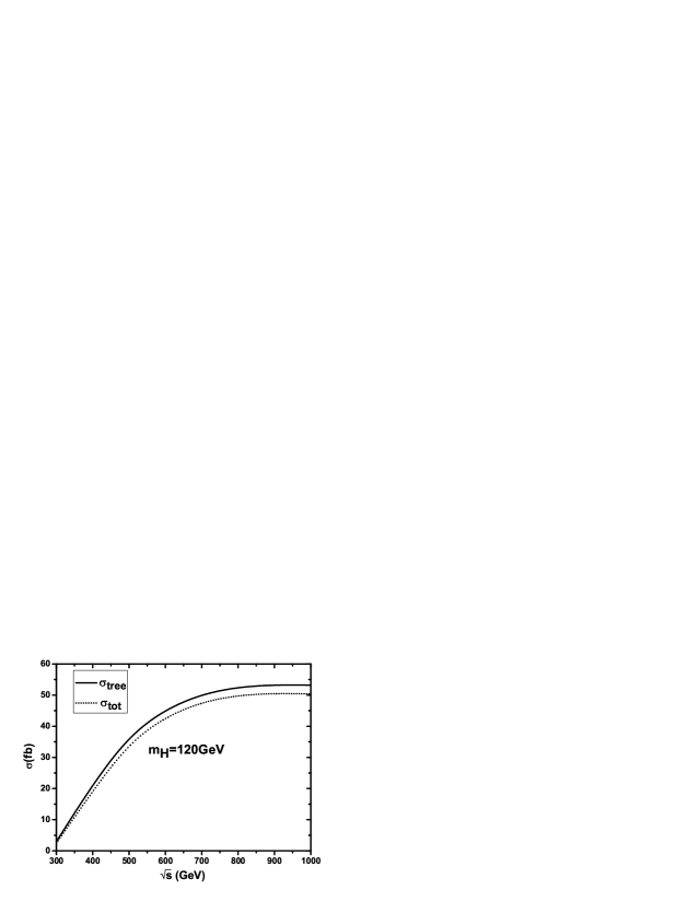
Figure 4: (a) The LO and EW NLO corrected cross sections for the process $e^{+}e^{-}\to W^{+}W^{-}Z^{0}$ as the functions of colliding energy $\sqrt{s}$ with $m_{H}=120~{}GeV$. (b) The corresponding EW relative radiative corrections versus $\sqrt{s}$.

$\sqrt{s}$ (GeV)	$m_{H}(GeV)$	$\sigma_{tree}(fb)$	$\sigma_{tot}(fb)$	$\Delta\sigma_{tot}(fb)$	$\delta_{ew}($%$)$
300	120	2.9457(2)	2.427(2)	-0.519(2)	-17.62(7)
300	150	3.1605(2)	2.633(2)	-0.527(2)	-16.67(6)
500	120	35.810(4)	33.51(5)	-2.30(5)	-6.4(1)
500	150	36.035(4)	33.85(5)	-2.19(5)	-6.1(1)
800	120	52.34(1)	49.70(6)	-2.64(5)	-5.0(1)
800	150	52.46(1)	50.10(6)	-2.36(6)	-4.5(1)
1000	120	53.21(1)	50.37(7)	-2.84(7)	-5.3(1)
1000	150	53.28(1)	50.70(7)	-2.58(7)	-4.8(1)

Table 2: The numerical results of the LO, EW NLO corrected cross sections, the EW NLO correction to the cross section ($\Delta\sigma_{tot}$) and the EW relative correction ($\delta_{ew}$) for the process $e^{+}e^{-}\to W^{+}W^{-}Z^{0}$ , in conditions of $m_{H}=120~{}GeV$, $150~{}GeV$ and $\sqrt{s}=300~{}GeV$, $500~{}GeV$, $800~{}GeV$, $1000~{}GeV$, separately.

Because the distribution of transverse momenta of $p_{T}^{W^{-}}$ is the same as that of $p_{T}^{W^{+}}$ in the CP-conserving SM, we provide only the distributions of $p_{T}^{W^{-}}$ at the LO and EW NLO in Fig.5(a). The differential cross sections of transverse momentum of $Z^{0}$-boson at the LO and up to NLO ($\frac{d\sigma_{LO}}{dp_{T}^{Z}}$ and $\frac{d\sigma_{NLO}}{dp_{T}^{Z}}$) are drawn in Fig.5(b). In these two figures we take $m_{H}=120~{}GeV$ and $\sqrt{s}=500~{}GeV$. We can see from Figs.5(a,b) that the EW NLO corrections generally suppress the LO differential cross sections especially when $p_{T}^{W^{-}}(p_{T}^{Z})>100~{}GeV$.

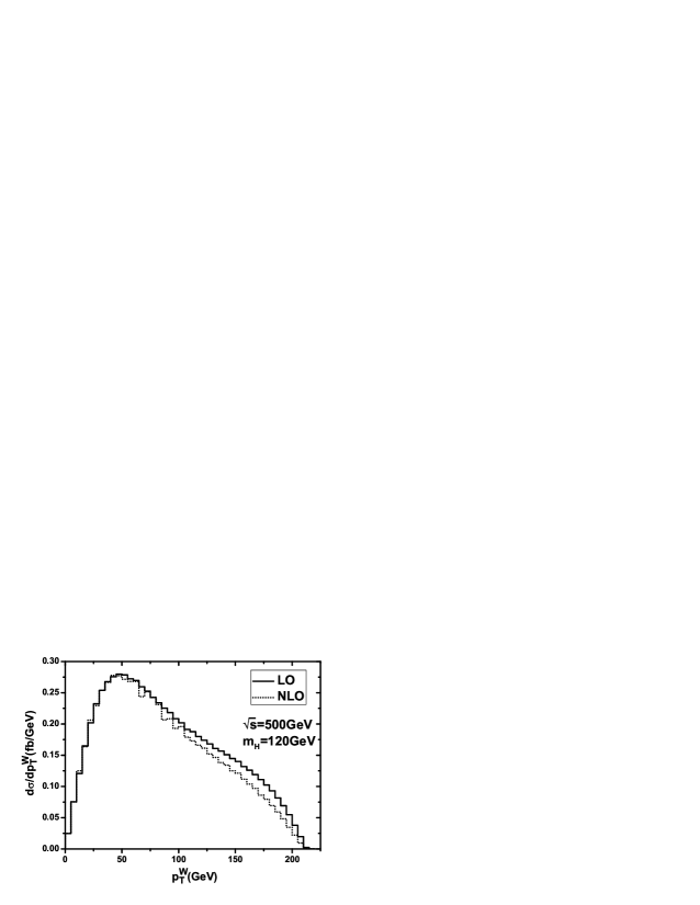
Figure 5: Distributions of the transverse momenta of $W^{-}$- and $Z^{0}$-boson for the $e^{+}e^{-}\to W^{+}W^{-}Z^{0}$ process at the LO and EW NLO with $\sqrt{s}=500~{}GeV$ and $m_{H}=120~{}GeV$. (a) for $W^{-}$-boson, (b) for $Z^{0}$-boson.

We take the orientation of incoming electron as the z-axis. The $\theta_{W^{-}}$ (or $\theta_{Z}$) is defined as the $W^{-}$-boson (or $Z^{0}$-boson) production angle with respect to the z-axis. In Figs.6(a,b) we present the LO and EW NLO distributions of cosines of the pole angles of $W^{-}$- and $Z^{0}$-boson($\cos\theta_{W^{-}}$ and $\cos\theta_{Z}$) respectively, in conditions of $\sqrt{s}=500~{}GeV$ and $m_{H}=120~{}GeV$. Both LO and NLO curves in Fig.6(a) show that the produced $W^{-}$-boson declines to go out in the forward hemisphere, while Fig.6(b) demonstrates that the LO and NLO distributions of the outgoing $Z^{0}$-boson are symmetry in the forward and backward hemisphere regions.

The distributions of the $W$-pair invariant mass $M_{WW}$ at the LO and EW NLO are shown in Fig.7(a), and the differential cross sections of the cosine of the angle between the produced $W$-pair at the LO and EW NLO are presented in Fig.7(b) where we take $m_{H}=120~{}GeV$ and $\sqrt{s}=500~{}GeV$. We can see from the Fig.7(a) that there is an enhancement in the relatively large $M_{WW}$ region(from $350~{}GeV$ to $400~{}GeV$) for each of the LO and NLO distributions, and the EW NLO correction suppresses significantly the LO differential cross section $d\sigma_{LO}/dM_{WW}$ in this region. Fig.7(b) shows the LO and EW NLO distributions of cosine of the angle between the produced $W$-pair. And we can see from the figure that the produced $W$-pair prefer to go out almost back to back, that leads to the $M_{WW}$ having the tendency to distribute in large value region. That is why we see an enhancement in the large $M_{WW}$ region for each of the LO and NLO distributions as shown in Fig.7(a).

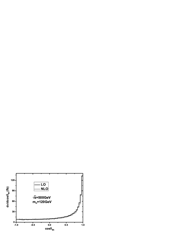
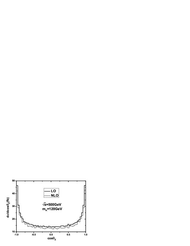
Figure 6: Distributions of the cosine of the $W^{-}$-boson ($Z^{0}$-boson) production angle with respect to z-axis for the $e^{+}e^{-}\to W^{+}W^{-}Z^{0}$ process at the LO and EW NLO with $\sqrt{s}=500~{}GeV$ and $m_{H}=120~{}GeV$. (a) for $\frac{d\sigma_{LO,NLO}}{d\cos\theta_{W^{-}}}$, (b) for $\frac{d\sigma_{LO,NLO}}{d\cos\theta_{Z}}$.

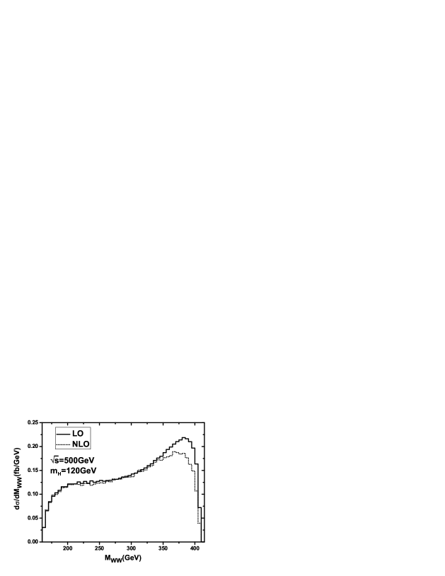
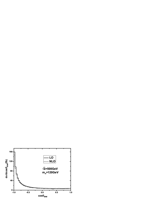
Figure 7: (a) Distributions of the invariant mass of $W$-pair at the LO and EW NLO when $m_{H}=120~{}GeV$ and $\sqrt{s}=500~{}GeV$. (b) Differential cross sections of the cosine of the angle between the produced $W$-pair at the LO and EW NLO with $m_{H}=120~{}GeV$ and $\sqrt{s}=500~{}GeV$.

On the analogy of the definitions of the LO and NLO forward-backward charge asymmetry for top-quark in Ref.[27], we define the LO and NLO forward-backward charge asymmetries of $W^{-}$-boson as,

$$A_{FB,LO}^{W^{-}}=\frac{\sigma_{tree}^{-}}{\sigma_{tree}^{+}},~{}~{}~{}~{}~{}A_{FB,NLO}^{W^{-}}=\frac{\sigma_{tree}^{-}}{\sigma_{tree}^{+}}\left(1+\frac{\Delta\sigma_{tot}^{-}}{\sigma_{tree}^{-}}-\frac{\Delta\sigma_{tot}^{+}}{\sigma_{tree}^{+}}\right).$$ (3.2)

The explicit expressions for $\sigma_{tree}^{\pm}$ are defined as

$$\sigma_{tree}^{\pm}=\sigma_{tree}(y_{W^{-}}>0)\pm\sigma_{tree}(y_{W^{-}}<0),$$ (3.3)

where $y_{W^{-}}$ is the rapidity of $W^{-}$-boson, the notations $\sigma_{tree}(y_{W^{-}}>0)$ and $\sigma_{tree}(y_{W^{-}}<0)$ represent the cross sections for the produced $W^{-}$-bosons in the forward and backward hemispheres at the LO respectively. The forward direction is along the orientation of z-axis. $\Delta\sigma_{tot}^{\pm}$ denote the EW NLO corrections to the cross sections $\sigma^{\pm}_{tree}$. In the conditions of $\sqrt{s}=500~{}GeV$ and $m_{H}=120~{}GeV$, we get $A_{FB,LO}^{W^{-}}=50.98(2)\%$ and $A_{FB,NLO}^{W^{-}}=53.28(3)\%$. Both the LO and NLO results show that most of the $W^{-}$-bosons are produced in the forward hemisphere, that feature has been already demonstrated in Fig.6(a).

IV. Summary

The $W^{+}W^{-}Z^{0}$ production via electron-positron collision at the ILC is an important process not only in probing the non-Abelian structures of the SM, but also in finding new physics. In this report we have shown that the phenomenological effects due to the one-loop EW radiative corrections, can be demonstrated in the $e^{+}e^{-}\to W^{+}W^{-}Z^{0}$ process for all colliding energies ranging from $300~{}GeV$ to $1~{}TeV$ at the ILC. Our results show the EW one-loop radiative corrections significantly suppress the LO cross sections, and the relative correction to the cross section varies from $-17.6\%$ to $-5.3\%$ when $m_{H}=120~{}GeV$ and $\sqrt{s}$ goes up from $300~{}GeV$ to $1~{}TeV$. We can see the obvious effects of the EW NLO correction on the physical observables, such as, the distributions of the transverse momenta of final $Z^{0}$- and $W$-bosons, the differential cross section of the invariant mass of $W$-pair, the distribution of the angle between $W$-pair, the production pole angle distributions of $W^{-}$- and $Z^{0}$-boson, and the forward-backward charge asymmetry of $W^{-}$-boson.

Acknowledgments: This work was supported in part by the National Natural Science Foundation of China(No.10875112, No.10675110), the National Science Fund for Fostering Talents in Basic Science(No.J0630319).

References

- [1] S. L. Glashow, Nucl. Phys. 22 (1961) 579; S. Weinberg, Phys. Rev. Lett. 1 (1967) 1264; A. Salam, Proc. 8th Nobel Symposium Stockholm 1968,ed. N. Svartholm (Almquist and Wiksells, Stockholm 1968) p.367; H. D. Politzer, Phys. Rep. 14 (1974) 129.
- [2] P. W. Higgs, Phys. Lett 12 (1964) 132, Phys. Rev. Lett. 13 (1964) 508; Phys. Rev. 145 (1966) 1156; F. Englert and R.Brout, Phys. Rev. Lett. 13 (1964) 321; G. S. Guralnik, C. R. Hagen and T. W. B. Kibble, Phys. Rev. Lett. 13 (1964) 585; T. W. B. Kibble, Phys. Rev. 155 (1967) 1554.
- [3] G. Gounaris et al., in Physics at LEP 2, Report CERN 96-01 (1996), eds G. Altarelli, T. Sjöstrand, F. Zwirner, Vol. 1, 525.
- [4] The LEP Collaborations, A combination of preliminary electroweak measurements and constraints on the standard model, CERN-PH-EP/2004-069, arXiv: hep-ex/0412015v2.
- [5] M. Lemoine and M. J. G. Veltman, Nucl. Phys. B164 (1980) 445; M. Bohm, A. Denner, T. Sack, W. Beenakker, F. A. Berends and H. Kuijf, Nucl. Phys. B304 (1988) 463; J. Fleischer, F. Jegerlehner and M. Zralek, Z. Phys. C42 (1989) 409; W. Beenakker, A. Denner, S. Dittmaier, R. Mertig and T. Sack, Nucl. Phys. B410 (1993) 245; A. Denner, S. Dittmaier, M. Roth and L. H. Wieders, Phys. Lett. B612 (2005) 223; Nucl. Phys. B724 (2005) 247.
- [6] W. Beenakker, F. A. Berends and A. P. Chapovsky, Nucl. Phys. B548 (1999) 3.
- [7] J. H. Kühn, F. Metzler and A. A. Penin, Nucl. Phys. B795 (2008) 277.
- [8] Mark S. Neubauer, FERMILAB-CONF-06-115-E, arXiv: hep-ex/0605066v2; Junjie Zhu, arXiv: 0907.3239v1; The D0 Collaboration, V. Abazov, et al., Combined measurements of anomalous charged trilinear gauge-boson couplings from diboson production in collisions at TeV, FERMILAB-PUB-09-380-E, arXiv: 0907.4952v1.
- [9] A. Lazopoulos, K. Melnikov and F. Petriello, Phys. Rev. D76 (2007) 014001; V. Hankele and D. Zeppenfeld, Phys. Lett. B661 (2008) 103; T. Binoth, G. Ossola, C. G. Papadopoulos and R. Pittau, JHEP 0806 (2008) 082.
- [10] Parameters for Linear Collider, http://www.fnal.gov/directorate/icfa/LC_parameters.pdf
- [11] Su Ji-Juan, Ma Wen-Gan, Zhang Ren-You, Wang Shao-Ming and Guo Lei, Phys. Rev. D78 (2008) 016007.
- [12] V. Barger, T. Han and R. J. N. Phillips, Phys. Rev. D39 (1989) 146; C. Grosse-Knetter and D. Schildknecht, Phys. Lett. B302 (1993) 309; S. Dawson, A. Likhoded, G. Valencia and O. Yushchenko, arXiv: hep-ph/9610299; T. Han, H. -J. He and C. -P. Yuan, Phys. Lett. B422 (1998) 294; M. Beyer, S. Christ, E. Schmidt and H. Schroeder, arXiv: hep-ph/0409305.
- [13] T. Hahn, Comput. Phys. Commun. 140 (2001) 418.
- [14] T. Hahn, M. Perez-Victoria, Comput. Phys. Commun. 118 (1999) 153.
- [15] A. Denner, Fortschr. Phys. 41 (1993) 307.
- [16] G. ’t Hooft and M. Veltman, Nucl. Phys. B44 (1972) 189.
- [17] D. A. Ross and J. C. Taylor, Nucl. Phys. B51 (1979) 25.
- [18] G. Passarino and M. Veltman, Nucl. Phys. B160 151 (1979).
- [19] A. Denner and S. Dittmaier, Nucl. Phys. B658 (2003) 175.
- [20] G.’t Hooft and M. Veltman, Nucl. Phys. B153 (1979) 365.
- [21] A. Denner, U Nierste and R Scharf, Nucl. Phys. B367 (1991) 637.
- [22] G. J. van Oldenborgh, Comput. Phys. Commun 58 (1991) 1.
- [23] C. Amsler, et al., Phys. Lett. B667 (2008) 1.
- [24] T. Kinoshita, J. Math. Phys. 3 (1962) 650; T. D. Lee and M. Nauenberg, Phys. Rev. 133 (1964) 1549.
- [25] B. W. Harris and J. F. Owens, Phys. Rev. D65 (2002) 094032.
- [26] F. Jegerlehner, Report No. DESY 01-029, arXiv: hep-ph/0105283.
- [27] S. Dittmaier, P. Uwer and S. Weinzierl, Eur. Phys. J. C59 (2009) 625.