Influence of energetically close orbitals on molecular high-order harmonic generation

Abstract

We investigate the contributions from the $3\sigma_{g}$ and $1\pi_{u}$ and molecular orbitals in high-order harmonic generation in $N_{2}$, with particular emphasis on quantum-interference effects. We consider both the physical processes in which the electron is freed and returns to the same orbital, and those in which it is ionized off one orbital and recombines with the other. We show that the quantum-interference patterns observed in the high-order harmonic spectra are predominantly determined by the $3\sigma_{g}$ orbital. This holds both for the situation in which only the $1\pi_{ux}$ orbital is considered, and the dynamics of the electron is restricted to the plane $p_{x}p_{z},$ or in the full three-dimensional case, if the azimuthal angle is integrated over and the degeneracy of $1\pi_{u}$ is taken into account.

I Introduction

In the past few years, high-order harmonic generation (HHG) has been extensively studied as a tool for attosecond imaging. In particular the possibility of bound-state reconstruction Itatani , the attosecond probing of dynamic processes in molecules attomol and quantum interference effects interfexp has attracted a great deal of attention. This is a consequence of the fact that HHG is the result of the recombination of an electron, freed by tunneling or multiphoton ionization at an instant $t^{\prime}$, with its parent molecule at a later instant $t$ tstep . Since, in principle, the electron may recombine with more than one center, high-harmonic emission at spatially separated sites takes place. Hence, information about the structure of the molecule in question is hidden in the HHG spectrum. In particular for diatomic molecules, this can be thought of as a microscopic counterpart of the double-slit experiment, in which maxima and minima arise due to the two-center interference doubleslit .

In many studies so far, it has been assumed that the electron is released from the highest-occupied molecular orbital (HOMO)MadsenN2 ; DM2009 ; DM2006 ; UsachenkoN2ion ; MoreN2 ; LinN2 ; McFar2008 . This, however, has been disputed in recent investigations, in which it was shown that multielectron effects and the quantum interference of different ionization channels may play an important role Multielectron . Such effects may constitute a serious obstacle towards ultra-fast molecular imaging. Apart from that, even if only the HOMO is considered as the initial state of the ionized electron, in many cases its degeneracy has a considerable influence on the HHG spectra degeneracy .

In this paper, we investigate the influence of different molecular orbitals on the high-order harmonic spectra of diatomic nitrogen $(N_{2})$. High-order harmonic generation MadsenN2 ; DM2009 ; Itatani ; Multielectron ; MoreN2 ; LinN2 and above-threshold ionization MadsenN2 ; UsachenkoN2ion ; DM2006 in $N_{2}$ have been extensively investigated in the literature, as, due to its large mass, its vibrational degrees of freedom do not play a very important role and may be ignored to first approximation. In fact, it has been shown that, whereas for lighter species, vibration may lead to a considerable blurring of the two-center interference patterns, and a reduction in the high-harmonic or photoelectron yield, for molecular nitrogen such effects are not significant MadsenN2 .

Furthermore, in $N_{2},$ the HOMO and the HOMO-1 orbitals are energetically very close. This has several consequences. First, since they possess opposite parity, one expects a strong coupling between them. Second, since the tunneling probability is related to the bound-state energy, the processes in which the electron starts in the HOMO and in the HOMO-1 are comparable. Third, the electron may also leave from one orbital and recombine with the other, and, quantum mechanically, the transition amplitude related to all physical processes involved will interfere. The influence of the HOMO-1 in the high-harmonic spectra of $N_{2}$ has been recently observed McFar2008 .

One should note, however, that, for $N_{2}$, the HOMO and the HOMO-1 exhibit very distinct shapes and symmetry. In fact, the former is a $3\sigma_{g}$ orbital and the latter a $1\pi_{u}$ orbital. Therefore, they are expected to behave differently as the alignment angle of the molecule with regard to the laser-field polarization is varied. Apart from that, the $1\pi_{u}$ orbital is doubly degenerate.

In our investigations, we employ the strong-field approximation hhgsfa , and saddle-point methods. The transition amplitudes obtained within this framework can be related to the classical orbits of an electron in a time-dependent field, and, yet, they retain information on the quantum interference between the possible physical processes orbitshhg . Throughout, we employ the length gauge. Even though there is considerable debate about which gauge to employ, and the length gauge SFA leads to potential-energy shifts whose meaning are not clear gauge , it has been recently shown that the two-center interference patterns are absent in SFA computations of the high-harmonic spectra using the velocity-gauge F2007 ; SSY2007 ; DM2009 .

This paper is organized as follows. In Sec. II, we provide the SFA transition amplitudes for the physical processes involved, for an exponential basis set involving Slater-type orbitals, and for a split-valence, gaussian basis set. Subsequently, in Sec. III, we compare the high-harmonic spectra obtained using both basis sets (Sec. III.1), and investigate quantum-interference effects between the $3\sigma_{g}$ and $1\pi_{u}$ orbital (Sec. III.2). Finally, in Sec. IV we summarize the paper and state our main conclusions.

II Transition amplitudes

Below we provide the HHG transition amplitudes, within the strong-field approximation. We base our approach on the explicit expression in Ref. hhgsfa , and employ atomic units throughout.

The HHG amplitude is generalized to the case in which the active electron is initially in a coherent superposition of the $3\sigma_{g}$ and the $1\pi_{u}$ orbitals.

Explicitly,

$$\left|\psi_{0}\right\rangle=C_{3\sigma_{g}}\left|3\sigma_{g}\right\rangle+C_{1\pi_{ux}}\left|1\pi_{ux}\right\rangle+C_{1\pi_{uy}}\left|1\pi_{uy}\right\rangle,$$

where the coefficients $C_{3\sigma_{g}}$, $C_{1\pi_{ux}}$ and $C_{1\pi_{uy}}$ give the weights of each state. One should note that the orbitals $1\pi_{ux}$ and $1\pi_{uy}$ are degenerate, and possess the energy $E_{1\pi u}$. In the present model, we will neglect the processes in which the electron, immediately before ionization, is excited from the $1\pi_{u}$ state to $3\sigma_{g},$ and, upon recombination, decays from $3\sigma_{g}$ to $1\pi_{u}.$

Under these assumptions, the overall transition amplitude will be the sum

$$M=\sum\limits_{j,\nu}M_{j\nu}+c.c.$$ (1)

of nine terms. Explicitly,

$$M_{11} = -i\left|C_{3\sigma_{g}}\right|^{2}\int_{-\infty}^{+\infty}dt\int\limits_{-\infty}^{t}dt^{\prime}\int d^{3}pd_{z}^{\ast(3\sigma_{g})}(\mathbf{p}+\mathbf{A}(t))$$ (2)

$$\times d_{z}^{(3\sigma_{g})}(\mathbf{p}+\mathbf{A}(t^{\prime}))\exp[iS_{11}(t,t^{\prime},\mathbf{p})],$$

$$M_{12} = -iC_{3\sigma_{g}}^{\ast}C_{1\pi_{ux}}\int_{-\infty}^{+\infty}dt\int\limits_{-\infty}^{t}dt^{\prime}\int d^{3}pd_{z}^{\ast(3\sigma_{g})}(\mathbf{p}+\mathbf{A}(t))$$ (3)

$$\times d_{z}^{(1\pi_{ux})}(\mathbf{p}+\mathbf{A}(t^{\prime}))\exp[iS_{12}(t,t^{\prime},\mathbf{p})],$$

$$M_{13} = -iC_{3\sigma_{g}}^{\ast}C_{1\pi_{uy}}\int_{-\infty}^{+\infty}dt\int\limits_{-\infty}^{t}dt^{\prime}\int d^{3}pd_{z}^{\ast(3\sigma_{g})}(\mathbf{p}+\mathbf{A}(t))$$ (4)

$$\times d_{z}^{(1\pi_{uy})}(\mathbf{p}+\mathbf{A}(t^{\prime}))\exp[iS_{13}(t,t^{\prime},\mathbf{p})],$$

$$M_{21} = -iC_{3\sigma_{g}}C_{1\pi_{ux}}^{\ast}\int_{-\infty}^{+\infty}dt\int\limits_{-\infty}^{t}dt^{\prime}\int d^{3}pd_{z}^{\ast(1\pi_{ux})}(\mathbf{p}+\mathbf{A}(t))$$ (5)

$$\times d_{z}^{(3\sigma_{g})}(\mathbf{p}+\mathbf{A}(t^{\prime}))\exp[iS_{21}(t,t^{\prime},\mathbf{p})],$$

$$M_{22} = -i\left|C_{1\pi_{ux}}\right|^{2}\int_{-\infty}^{+\infty}dt\int\limits_{-\infty}^{t}dt^{\prime}\int d^{3}pd_{z}^{\ast(1\pi_{ux})}(\mathbf{p}+\mathbf{A}(t))$$ (6)

$$\times d_{z}^{(1\pi_{ux})}(\mathbf{p}+\mathbf{A}(t^{\prime}))\exp[iS_{22}(t,t^{\prime},\mathbf{p})],$$

$$M_{23} = -iC_{1\pi_{ux}}^{\ast}C_{1\pi_{uy}}\int_{-\infty}^{+\infty}dt\int\limits_{-\infty}^{t}dt^{\prime}\int d^{3}pd_{z}^{\ast(1\pi_{ux})}(\mathbf{p}+\mathbf{A}(t))$$ (7)

$$\times d_{z}^{(1\pi_{uy})}(\mathbf{p}+\mathbf{A}(t^{\prime}))\exp[iS_{23}(t,t^{\prime},\mathbf{p})],$$

$$M_{31} = -iC_{3\sigma_{g}}C_{1\pi_{uy}}^{\ast}\int_{-\infty}^{+\infty}dt\int\limits_{-\infty}^{t}dt^{\prime}\int d^{3}pd_{z}^{\ast(1\pi_{uy})}(\mathbf{p}+\mathbf{A}(t))$$ (8)

$$\times d_{z}^{(3\sigma_{g})}(\mathbf{p}+\mathbf{A}(t^{\prime}))\exp[iS_{31}(t,t^{\prime},\mathbf{p})],$$

$$M_{32} = -iC_{1\pi_{uy}}^{\ast}C_{1\pi_{ux}}\int_{-\infty}^{+\infty}dt\int\limits_{-\infty}^{t}dt^{\prime}\int d^{3}pd_{z}^{\ast(1\pi_{uy})}(\mathbf{p}+\mathbf{A}(t))$$ (9)

$$\times d_{z}^{(1\pi_{ux})}(\mathbf{p}+\mathbf{A}(t^{\prime}))\exp[iS_{32}(t,t^{\prime},\mathbf{p})],$$

$$M_{33} = -i\left|C_{1\pi_{uy}}\right|^{2}\int_{-\infty}^{+\infty}dt\int\limits_{-\infty}^{t}dt^{\prime}\int d^{3}pd_{z}^{\ast(1\pi_{uy})}(\mathbf{p}+\mathbf{A}(t))$$ (10)

$$\times d_{z}^{(1\pi_{uy})}(\mathbf{p}+\mathbf{A}(t^{\prime}))\exp[iS_{33}(t,t^{\prime},\mathbf{p})],$$

where $d_{z}^{(3\sigma_{g})}(\mathbf{p})=\left\langle\mathbf{p}\right|\mathbf{r}.\hat{e}_{z}\left|3\sigma_{g}\right\rangle$ and $d_{z}^{(1\pi_{u\xi})}(\mathbf{p})=\left\langle\mathbf{p}\right|\mathbf{r}.\hat{e}_{z}\left|1\pi_{u\xi}\right\rangle,(\xi=x,y)$ are the components of the dipole matrix elements related to $3\sigma_{g}$ and $1\pi_{u}$ along the field-polarization axis.

In the above-stated equations, one may distinguish two types of contributions. The amplitudes $M_{jj}$ correspond to the processes in which the electron leaves a specific orbital, reaches a Volkov state $\left|\mathbf{p}+\mathbf{A}(t^{\prime})\right\rangle$, propagates in the continuum from $t^{\prime}$ to $t$, and recombines from a Volkov state $\left|\mathbf{p}+\mathbf{A}(t)\right\rangle$ to the same orbital it left from. The amplitudes $M_{j\nu},$ $j\neq\nu,$ on the other hand, give the processes in which the electron leaves from one orbital and returns to another. The corresponding actions read

$$S_{jj}(t,t^{\prime},\mathbf{p})=S(t,t^{\prime},\mathbf{p})-E_{\alpha}(t-t^{\prime}),$$ (11)

and

$$S_{j\nu}(t,t^{\prime},\mathbf{p})=S(t,t^{\prime},\mathbf{p})-(E_{\alpha}t-E_{\beta}t^{\prime}),\ j\neq\nu,$$ (12)

respectively, with

$$S(t,t^{\prime},\mathbf{p})=\Omega t-\frac{1}{2}\int_{t^{\prime}}^{t}d\tau\left[\mathbf{p}+\mathbf{A}(\tau)\right]^{2}.$$ (13)

In the above-stated equations, $E_{\alpha},E_{\beta}$ refer to the bound-state energies, $t$ to the recombination time, $t^{\prime}$ to the start time and $\mathbf{p}$ the intermediate momentum. For  $S_{11},\alpha=3\sigma_{g},$ while for  $S_{22}$ and $S_{33},\alpha=1\pi_{u}$. For $S_{12}(t,t^{\prime},\mathbf{p}),$ $E_{\alpha}=E_{3\sigma_{g}}$ and $E_{\beta}=E_{1\pi_{u}},$whilst, for $S_{21}(t,t^{\prime},\mathbf{p}),$ the situation is reversed, i.e., $E_{\alpha}=E_{{}_{1\pi_{u}}}$ and $E_{\beta}=E_{3\sigma_{g}}$. Note that, due to the fact that the $1\pi_{u}$ orbitals are degenerate, $S_{12}=S_{13},$ $S_{21}=S_{31}$ and $S_{32}=S_{22}=S_{33}=S_{23}.$

We will compute the transition amplitude $M$ employing the stationary phase approximation, i.e., we will look for values of $t,t^{\prime}$ and $\mathbf{p}$ that renders the actions in Eqs. (2)-(6) stationary. Apart from considerably simplifying the computations involved, this approach provides a physical interpretation of the amplitudes $M_{j\nu}$ in terms of electron trajectories. We compute the transition amplitudes employing a uniform saddle-point approximation. Details on the specific method used can be found in atiuni .

II.1 Saddle-point equations

Differentiating $S_{11}$, $S_{22}$ and $S_{33}$ with respect to the ionization time $t^{\prime}$ and the recombination time $t,$ we obtain the saddle-point equations

$$\frac{\left[\mathbf{p}+\mathbf{A}(t^{\prime})\right]^{2}}{2}+E_{\alpha}=0$$ (14)

and

$$\frac{\left[\mathbf{p}+\mathbf{A}(t)\right]^{2}}{2}+E_{\alpha}=\Omega,$$ (15)

where $\alpha=3\sigma_{g}$ for $S_{11}(t,t^{\prime},\mathbf{p})$ and $\alpha=1\pi_{u}$ for $S_{22}$ and $S_{33}.$ Physically, Eq. (14) gives the conservation of energy at the instant of tunneling, and Eq. (15) expresses the fact that the electron recombines to the same state (either $\left|3\sigma_{g}\right\rangle$ or $\left|1\pi_{u}\right\rangle$), releasing its kinetic energy upon return in form of a high-order harmonic of frequency $\Omega$. Finally, the condition $\partial S_{jj}/\partial\mathbf{p}=\mathbf{0}$ yields

$$\int_{t^{\prime}}^{t}d\tau\left[\mathbf{p}+\mathbf{A}(\tau)\right]=\mathbf{0}$$ (16)

Eq. (16) constrains the intermediate momentum of the electron, so that it returns to the site of its release. In the present model, this site is taken as the origin of our coordinate system, and is the geometric center of the molecule. Summarizing, the saddle-point equations (14)-(16) are related to the physical picture of an electron ionizing from either the HOMO or the HOMO-1 in $N_{2}$ and returning to the same state.

The remaining actions $S_{j\nu}(t,t^{\prime},\mathbf{p}),$ for $j\neq\nu,$ lead to the saddle-point equations

$$\frac{\left[\mathbf{p}+\mathbf{A}(t^{\prime})\right]^{2}}{2}+E_{\beta}=0$$ (17)

and

$$\frac{\left[\mathbf{p}+\mathbf{A}(t)\right]^{2}}{2}+E_{\alpha}=\Omega,$$ (18)

which indicate that the electron has left from one state and recombined with the other. For $S_{12}(t,t^{\prime},\mathbf{p})$ and $S_{13}(t,t^{\prime},\mathbf{p}),$ $E_{\alpha}=E_{3\sigma_{g}}$ and $E_{\beta}=E_{1\pi_{u}},$while, for $S_{21}(t,t^{\prime},\mathbf{p})$ and $S_{31}(t,t^{\prime},\mathbf{p}),$ the situation is reversed, i.e., $E_{\alpha}=E_{{}_{1\pi_{u}}}$ and $E_{\beta}=E_{3\sigma_{g}}$. For the remaining terms, $E_{\alpha}=E_{\beta}=E_{{}_{1\pi_{u}}}$ so that Eqs. (14) and (15) are recovered. Physically, this corresponds to the situation in which the electron leaves $\left|1\pi_{ux}\right\rangle$ and returns to $\left|1\pi_{uy}\right\rangle,$ or vice-versa. The return condition (16) remains the same in this case.

II.2 Orbital wavefunctions and dipole matrix elements

Within the framework of the strong-field approximation, all structural information about the molecule is embedded in the recombination prefactor $d_{z}^{(\Psi)}(\mathbf{p+A}(t))=\left\langle\mathbf{p+A}(t)\right|\mathbf{r}.\hat{e}_{z}\left|\Psi\right\rangle,$ with $\Psi=3\sigma_{g}$ or $1\pi_{u}.$ In position space, this prefactor is given by

$$d_{z}^{(\Psi)}(\mathbf{p})=\frac{1}{(2\pi)^{3/2}}\int d^{3}r\mathbf{p}\cdot\hat{e}_{z}\exp[-i\mathbf{p}\cdot\mathbf{r}]\Psi(\mathbf{r}),$$ (19)

i.e., the component of $i\partial_{\mathbf{p}}\Psi(\mathbf{p})$ along the laser-field polarization. In the following, we will construct  the momentum-space wavefunction $\Psi(\mathbf{p})$ for both orbitals. We will consider the linear combination of atomic orbitals (LCAO) approximation and frozen nuclei. This implies that the position-space wavefunction reads

$$\Psi(\mathbf{r})=\sum_{a}\psi_{a}(\mathbf{r+R}/2)+(-1)^{l_{a}-m_{a}+\lambda_{a}}\psi_{a}(\mathbf{r-R}/2),$$ (20)

where $\mathbf{R,}$ $l_{a}$ and $m_{a}$ denote the internuclear separation, the orbital and magnetic quantum numbers, respectively. For gerade and ungerade symmetry, $\lambda_{a}=\left|m_{a}\right|$ and $\lambda_{a}=\left|m_{a}\right|+1$, respectively.

Throughout, we will use the length form of the dipole operator and neglect the terms growing linearly with the internuclear separation. Such terms are artifacts and come from the lack of orthogonality between the Volkov states and the field-free bound states. For a more complete discussion see dressedSFA ; JMOCL2006 ; F2007 .

The wave functions $\psi_{a}(\mathbf{r})$ will be approximated by either exponentially decaying, Slater-type orbitals or by a gaussian basis set. In the former case,

$$\psi_{a}^{(HF)}(\mathbf{r})=\frac{c_{a}(2\zeta_{a})^{n_{a}+1/2}}{\sqrt{(2n_{a})!}}r^{n_{a}-1}e^{-\zeta_{a}r}Y_{l_{a}}^{m_{a}}(\theta,\phi),$$ (21)

where $n_{a}$ refers to the principal quantum number, and, in the latter,

$$\psi_{a}^{(G)}(\mathbf{r})=\sum\limits_{j}\tilde{c}_{aj}\varphi_{j}^{(G)}(\mathbf{r})$$ (22)

with

$$\varphi_{j}^{(G)}(\mathbf{r})=\sum_{\nu}b_{\nu}x^{\beta_{x}}y^{\beta_{y}}z^{\beta_{z}}\exp[-\zeta_{\nu}r^{2}].$$ (23)

The coefficients $c_{a},$ $\tilde{c}_{aj}$ and $b_{\nu}$ and the exponents $\zeta$ are extracted either from quantum chemistry codes, or from existing literature.

An exponential basis set has been recently employed in the literature MadsenN2 ; DM2006 ; DM2009 , while the use of gaussians is more widespread within the quantum chemistry community. In particular, a gaussian basis set exhibits several advantages.

First, it allows an easier evaluation of the momentum-space wavefunction, which will be a central ingredient for computing the matrix elements $d_{z}^{(\Psi)}(\mathbf{p+A}(t)).$ Second, within the SFA framework, for exponentially decaying states, the ionization prefactor $d_{z}^{(\Psi)}(\mathbf{p+A}(t^{\prime}))$ exhibits a singularity, according to the saddle-point equations (14) and (17). In previous work, we have eliminated this singularity by incorporating the prefactor $d_{z}^{(\Psi)}(\mathbf{p+A}(t^{\prime}))$ in the action, and found out that it did not play a considerable role singularity . This singularity, however, is absent if gaussian wavefunctions are taken. Finally, in Hartree Fock computations there is an artifact that renders the $1\pi_{u}$ orbital more loosely bound than $3\sigma_{g}.$

Explicitly, the Fourier transform of  Eq. (20) reads

$$\Psi(\mathbf{p})=\sum_{a}\eta(l_{a},m_{a},\mathbf{p}+\mathbf{A}(t))\psi_{a}(\mathbf{p}),$$ (24)

with

$$\eta(l_{a},m_{a},\mathbf{p})=\mathcal{C}_{+}\cos\left[\frac{\mathbf{p\cdot R}}{2}\right]+i\mathcal{C}_{-}\sin\left[\frac{\mathbf{p\cdot R}}{2}\right]$$ (25)

and

$$\mathcal{C}_{\pm}=\pm 1+(-1)^{l_{a}-m_{a}+\lambda_{a}}.$$ (26)

A generalized interference condition, which takes into account the structure of the orbitals in question, such as, for instance the $s$-$p$ mixing in the $3\sigma_{g}$ orbital, can be inferred from Eq. (24). Indeed, if we consider $\vartheta=\arctan(i\mathcal{C}_{+}/\mathcal{C}_{-}),$ then

$$\eta(l_{a},m_{a},\mathbf{p})=\sqrt{\mathcal{C}_{+}^{2}-\mathcal{C}_{-}^{2}}\sin[\vartheta+\mathbf{p\cdot R}/2].$$ (27)

For $\eta(l_{a},m_{a},\mathbf{p}+\mathbf{A}(t))$, interference minima are present if

$$\vartheta+[\mathbf{p}+\mathbf{A}(t)]\cdot\mathbf{R}/2=\kappa\pi,$$ (28)

where $\kappa$ denotes an integer number. This interference condition has been first derived in DM2009 .

For Slater-type orbitals the individual wavefunctions are given by

$$\psi_{a}^{(HF)}(\mathbf{p}) = \frac{(-ip)^{l_{a}}2^{n_{a}-l_{a}}\zeta_{a}^{-(l_{a}+3/2)}}{\sqrt{(2n_{a})!}}\frac{\Gamma(2+l_{a}+n_{a})}{\Gamma(3/2+n_{a})}$$ (29)

$$\times_{2}F_{1}(\alpha_{1},\alpha_{2},\alpha_{3},\alpha_{4})Y_{l_{a}}^{m_{a}}(\theta_{p},\phi_{p}),$$

and the arguments of the hypergeometric functions read $\alpha_{1}=$ $1+(l_{a}+n_{a})/2,$ $\alpha_{2}=$ $\alpha_{1}+1/2,$ $\alpha_{3}=l_{a}+3/2,\alpha_{4}=-p^{2}/\zeta_{a}^{2}.$ The angles are given by $\theta_{p}=\cos^{-1}(p_{z}/p)$ and $\phi_{p}=\tan^{-1}(p_{y}/p_{x})$.

It is worth noticing that Eq. (29) is mainly employed in the description of $\sigma$ orbitals, since the spherical harmonics $Y_{l_{a}}^{m_{a}}(\theta_{p},\phi_{p})$ are real for $m_{a}=0.$ For $\pi$ orbitals, it makes physically more sense to employ real spherical harmonics, which are linear combinations of $Y_{l_{a}}^{m_{a}}(\theta_{p},\phi_{p})$ and $Y_{l_{a}}^{-m_{a}}(\theta_{p},\phi_{p}).$ The explicit expressions for the real spherical harmonics are provided in DM2009 .

For a gaussian basis set the wavefunction $\psi_{a}(\mathbf{p})$ reads

$$\psi_{a}^{(G)}(\mathbf{p})=\sum\limits_{j,\nu}\tilde{c}_{aj}b_{\nu}\tilde{\varphi}_{\nu}(\mathbf{p}),$$ (30)

with

$$\tilde{\varphi}_{\nu}(\mathbf{p})=\prod\limits_{k}\tilde{\varphi}_{\nu}(p_{k})$$ (31)

and $k=x,y,z.$ Explicitly,

$$\tilde{\varphi}_{\nu}(p_{k})=\frac{1}{2}\zeta^{-\frac{\beta k}{2}-1}\left(\chi(p_{k})+\Xi(p_{k})\right),$$ (32)

$\tilde{\xi}$with

$$\chi(p_{k}) = i\left(-1+(-1)^{\beta_{k}}\right)p_{k}\Gamma\left(\xi_{k}+\frac{1}{2}\right)\,$$ (33)

$$\times_{1}F_{1}\left(\xi_{k}+\frac{1}{2};\frac{3}{2};\tilde{\xi}_{k}\right)$$

and

$$\Xi(p_{k})=\left(1+(-1)^{\beta_{k}}\right)\sqrt{\zeta_{\nu}}\Gamma\left(\xi_{k}\right)\,_{1}F_{1}\left(\xi_{k};\frac{1}{2};\tilde{\xi}_{k}\right).$$ (34)

The arguments of the Hypergeometric functions are denoted by $\xi_{k}=(\beta_{k}+1)/2$ and $\tilde{\xi}_{k}=-p_{k}^{2}/(4\zeta_{\nu}).$ In this work, we will be using $p$ and $s$ states, so that Eq. (31) will reduce to

$$\tilde{\varphi}_{\nu}(\mathbf{p})=(-ip_{k})^{l_{a}}\frac{\pi^{3/2}}{2^{l_{a}}\zeta_{\nu}^{3/2+l_{a}}}\exp[-p^{2}/(4\zeta_{\nu})].$$ (35)

Therein, $k=z,$ $k=x$ and $k=y$ for $\sigma,$ $\pi_{x}$ and $\pi_{y}$ states, respectively. The return condition (16) guarantees that the momentum $\mathbf{p}$ and the external field are collinear. Hence, for a linearly polarized field $\theta_{p}$ is equal to the alignment angle $\theta_{L}.$

III Harmonic spectra

In the following, we will present the high-order harmonic spectra. We choose the driving field as a linearly polarized monochromatic wave of frequency $\omega$ and amplitude $\omega A_{0}$ directed along the axis $z.$ Hence, the corresponding vector potential is

$$\mathbf{A}(t)=A_{0}\cos(\omega t)\hat{e}_{z}$$ (36)

For all situations, we consider starting times $0<t^{\prime}<\omega\pi$ confined to the first half cycle and the three shortest pairs of orbits. For this particular field, using the saddle-point equation (15), the generalized interference condition (28) may be expressed in terms of the harmonic order $n$ as

$$n=\frac{E_{\alpha}}{\omega}+\frac{2(\kappa-\vartheta)^{2}}{\omega R^{2}\cos^{2}\theta_{L}},$$ (37)

where $E_{\alpha}$ is the absolute value of the bound-state energy in question, $\kappa$ is an integer number, $\theta_{L}$ is the alignment angle, $R$ is the internuclear distance and $\vartheta$ is defined in Eq. (27).

III.1 HOMO and HOMO-1 contributions

In this section, we will make an assessment of the main differences encountered in the HHG spectra if the orbitals are built employing a split valence, gaussian basis set, or exponentially decaying, Slater-type orbitals. For that purpose, we will concentrate on the recombination prefactor $d_{z}^{(\Psi)}(\mathbf{p+A}(t))$ and assume that the ionization prefactor $d_{z}^{(\Psi)}(\mathbf{p+A}(t^{\prime}))$ is constant and unitary.

As a starting point, a direct comparison with the results reported in DM2009 for the $3\sigma_{g}$ orbital will be performed. This orbital is known to exhibit a strong mixing between $s$ and $p$ states. Therefore, we will address the question of how such a mixing influences the overall interference patterns. In the context of the present article, this implies that we will consider the transition amplitude $M_{11}$, for which the electron leaves and recombines with the $3\sigma_{g}$ orbital.

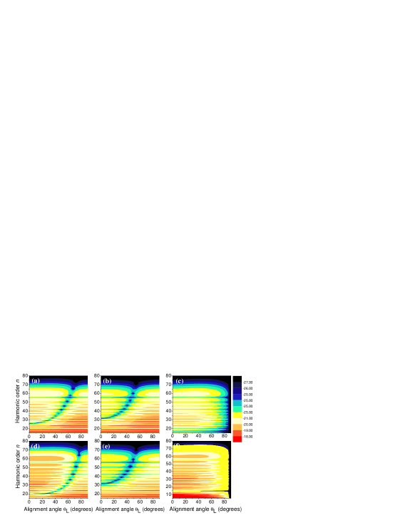
Figure 1: High-order harmonic spectra for the HOMO in $N_{2}$ subject to a linearly polarized laser field of frequency $\omega=0.057$ a.u. and intensity $I=4\times 10^{14}\mathrm{W/cm}^{2}$, as a function of the alignment angle $\theta_{L}$ between the molecule and the field. The spectra in the upper panels have been constructed using a gaussian basis set and coefficients obtained from GAMESS-UK GAMESS , while those in the lower panels have been built using Slater-type orbitals, and the coefficients in Cade66 . From left to right, we display the spectra from the full $3\sigma_{g}$ orbital [panels (a) and (d)], the contributions from the $s$ states [panels (b) and (e)], and those from the $p$ states [panels (c) and (f)]. The bound-state energy of the HOMO and the equilibrium internuclear distance have been taken from the respective computations. For the upper panels, $E_{3\sigma_{g}}=0.63485797$ a.u., while for the lower panels $E_{3\sigma_{g}}=0.63495$ a.u. In both cases, $R=2.068$ a.u.

In Fig. 1, we display such results, either computed with a 6-31G gaussian basis set and coefficients obtained from GAMESS-UK GAMESS , or with Slater-type orbitals (29), and the coefficients in Cade66 [upper and lower panels, respectively]. The outcome of the split-valence computation, displayed in Fig. 1.(a), exhibits a minimum which, for parallel molecular alignment, is near $\Omega=25\omega$. This is a slightly higher harmonic order than that observed in DM2009 (see Fig. 4 therein). The minima observed for the individual $s$ and $p$ contributions, in contrast, agree with the results presented in DM2009 (c.f. Fig. 1.(b) and Fig. 1.(c), respectively). This suggests that the $s$-$p$ mixing possesses different weights in the present case and in DM2009 .

The spectra obtained with the Slater-type orbitals, on the other hand, are practically identical to the results in DM2009 . This holds both for the minimum in the full $3\sigma_{g}$ spectrum [Fig. 1.(d)], which, for parallel alignment, is close to $\Omega=21\omega$, and for the patterns present in the $s$ and $p$ contributions [Fig. 1.(e) and Fig. 1.(f), respectively]. We have ruled out that this discrepancy is due to the slightly different ionization potentials employed in the two computations by performing a direct comparison for the same set of parameters (not shown). We have also found, employing GAMESS-UK and several types of basis sets, that the minimum at $\Omega=25\omega$ is rather robust with respect to small variations of $E_{3\sigma_{g}}$ and $R$. . Hence, in comparison to our computations, it seems that the contributions of the $s$ states to the spectra are slightly underestimated in Cade66 .

In Fig. 2, we present the high-harmonic spectra computed assuming, instead, that the electron comes back and returns to the $1\pi_{ux}$ orbital, i.e., employing the transition amplitude $M_{22}$. The $1\pi_{uy}$ orbital should behave in a similar way and lead to the same spectrum, as it exhibits the same dependence with regard to the alignment angle.

As in the $3\sigma_{g}$ case, we construct the bound-state wavefunction either from Slater-type orbitals and the data in Cade66 or from a 6-31G basis set obtained from GAMESS-UK GAMESS . These results are displayed in Figs. 2.(a) and 2.(b), respectively. In both cases, we find that the two-center interference occurs at the very same harmonic order. Furthermore, apart from discrepancies in the overall intensity, the spectra exhibit a very similar substructure. Finally, in both cases, the yield drops considerably for parallel-aligned molecules. This is expected, as, if the angle $\theta_{L}=0$, the $\pi$ orbitals exhibit a nodal plane along the polarization axis. If the alignment angle increases, this nodal plane moves further and further away from the field-polarization axis, and the high-order harmonic yield increases.

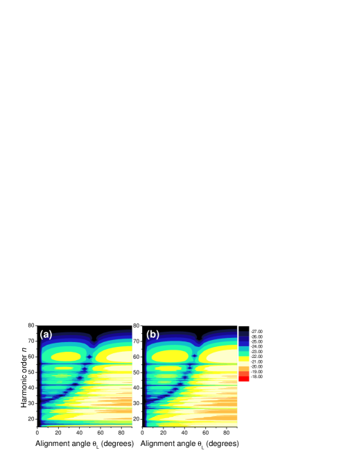
Figure 2: High-order harmonic spectra computed using the $1\pi_{ux}$ (HOMO-1) orbital in $N_{2}$ as a function of the alignment angle $\theta_{L}$, for the same laser-field parameters as in the previous figure. In panel (a), we considered a gaussian basis set and computed the coefficients with GAMESS-UK GAMESS , while in panel (b) we took Slater-type orbitals and the data from Cade66 . The bound-state energy of the HOMO and the equilibrium internuclear distance have been taken from the respective computations. For panel (a), $E_{1\pi_{u}}=0.61544$ a.u., while for panel (b) $E_{1\pi_{u}}=0.65087981$ a.u. In both cases, the internuclear distance is $R=2.068$. Note that in the Slater-type case the $1\pi_{u}$ orbitals are more loosely bound than the $3\sigma_{g}$ orbital.

III.2 Quantum interference of HOMO and HOMO-1

We will now investigate which signatures the interference between the $3\sigma_{g}$ and $1\pi_{u}$ leave on the high-order harmonic spectra. In all cases, we will consider both the recombination prefactor $d_{z}^{(\Psi)}(\mathbf{p+A}(t))$ and the ionization prefactor $d_{z}^{(\Psi)}(\mathbf{p+A}(t^{\prime}))$. The ionization prefactor is important in this context due to the fact that an electron reaching the continuum from a $\sigma$ or a $\pi$ orbital behaves in very different ways, with regard to the alignment angle $\theta_{L}$. In fact, for $\sigma$ orbitals, one expects ionization to be significant for small $\theta_{L}$ and to be negligible for large values of this parameter. For $\pi$ orbitals, due to the presence of the nodal plane, the opposite behavior is expected to occur.

III.2.1 Two-dimensional model

We will commence by addressing the situation for which $\phi_{p}=0$, i.e., we are restricting the dynamics of the problem to the $p_{x}p_{z}$ plane. In this case, the initial wavefunction is a superposition of the $3\sigma_{g}$ and $1\pi_{ux}$ states only, i.e., $C_{1\pi_{uy}}=0$. We consider that it is equally probable that the electron leaves from each of these states, i.e., $C_{3\sigma_{g}}=C_{1\pi_{ux}}=1/\sqrt{2}$.

In Fig. 3.(a), we show the full spectrum, in which all the transition amplitudes  $M_{j\nu},(j,\nu=1,2)$ are summed coherently. Especially for small alignment angles, this spectrum exhibits a minimum very close to that obtained if only the $3\sigma_{g}$ state is taken. This minimum gets more and more blurred as the alignment angle $\theta_{L}$ increases. Possibly, this is the main influence of the $1\pi_{ux}$ orbital, as its contributions increase with $\theta_{L}$. In the following, we will investigate these patterns in more detail. For that purpose, we consider the quantum interference between specific processes. These results are depicted in the remaining panels of Fig. 3.

If the electron recombines with the $1\pi_{ux}$ orbital, regardless of where it started from [Fig. 3.(b)], a very pronounced interference minimum is observed. This minimum occurs for the same harmonic orders as if only $\pi$ states are taken (c.f. Fig. 2). This is expected, as high-order harmonic generation in the former case is only due to recombination with the $1\pi_{ux}$ orbital, even if two orbitals are involved.

Apart from that, the yield practically vanishes at $\theta_{L}=0.$ This behavior is caused by the nodal plane which exists along the internuclear axis for the $\pi_{ux}$ orbital. In this case, recombination for both the transition amplitudes $M_{12}$ and $M_{22}$, and ionization for the transition amplitude $M_{22},$ are strongly suppressed. For parallel alignment, this plane is along the laser-field polarization. As the alignment angle increases, this plane moves away from the field-polarization axis. Consequently, the yield increases. This explains why, in the overall spectrum, the minimum is determined by the $3\sigma_{g}$ orbital. For the parameters considered in this work, such a minimum lies mostly in the region of small alignment angles.

In contrast, if only processes involving ionization from $1\pi_{ux}$ and recombination with $3\sigma_{g},$ or vice-versa, are taken, the double-slit interference minimum is completely blurred [c.f. Fig. 3.(c)]. This is due to the fact that both contributions are comparable, and exhibit minima for different harmonic orders. Furthermore, since either recombination with or ionization from a $\pi$ state is taking place, a strong suppression for $\theta_{L}=0$ is present. In Fig. 3, this is the only case for which we observed a complete disappearance of the double-slit minimum. Indeed, neither for the processes involving only one state [3.(d)], or starting at $3\sigma_{g}$ regardless of the end state [Fig. 3.(e)] does the minimum completely vanish. However, a sharp minimum is only present if we take into account the processes in which the electron recombines with the same state. Concrete examples are Fig. 3.(b), and Fig. 3.(f), where the processes finishing at $1\pi_{ux}$ and $3\sigma_{g}$, respectively, are presented. In Fig. 3.(f), we also notice that, for $0\leq\theta_{L}\leq 45^{\circ}$, the contributions from the $\sigma$ orbital are up to two orders of magnitude larger than those from the $\pi$ orbital [i.e., Fig. 3.(b)]. This is further evidence that the minimum is determined by the $3\sigma_{g}$ state.

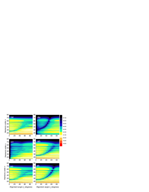
Figure 3: Contribution of different processes to the high-harmonic spectra, as functions of the alignment angle $\theta_{L}$, for the same field parameters in the previous figure. We chose $\phi_{p}=0$ so that the $1\pi_{uy}$ orbital does not contribute. The dipole matrix elements have been computed using a gaussian basis set and GAMESS-UK GAMESS . In this case, $E_{3\sigma_{g}}=0.63485797$ a.u, $E_{1\pi_{u}}=0.65087981$ a.u. and $R=2.068$ a.u. Panel (a): $|M_{11}+M_{22}+M_{12}+M_{21}|^{2}$; panel (b): processes finishing at the $1\pi_{ux}$ orbital, i.e., $|M_{21}+M_{22}|^{2}$; panel (c): processes in which the electron starts at one orbital and recombines with the other, i.e., $|M_{12}+M_{21}|^{2}$; panel (d): processes in which the electron starts from and returns to the same orbital, i.e., $|M_{11}+M_{22}|^{2}$; panel (e): processes starting at the $3\sigma_{g}$ orbital, i.e., $|M_{21}+M_{11}|^{2}$; panel (f): processes finishing at the $3\sigma_{g}$ orbital, i.e., $|M_{12}+M_{11}|^{2}$.

III.2.2 Three-dimensional case

In a more realistic situation, one cannot restrict the electron dynamics only to the $p_{x}p_{z}$ plane. In fact, there exist two $\pi$ orbitals which, even though they behave in the same way with respect to the alignment angle $\theta_{L},$ are degenerate. Hence, they provide a completely different weight to the states $\left|\psi_{0}\right\rangle$ from which the electron is released and to which it returns. Furthermore, under many experimental conditions, the azimuthal angle $\phi_{p}$ cannot be resolved. Thus, this parameter must be integrated over.

Explicitly, the resulting spectrum is given by

$$S(\Omega)=\int_{0}^{2\pi}|\sum\limits_{j,\nu}M_{j\nu}|^{2}d\phi_{p}.$$ (38)

For the specific problem addressed in this work, the above-stated sum consists of 81 terms. In general, the integrand in Eq (38) is of the form $M_{\alpha\beta}^{\ast}M_{j\nu}.$ Its general dependence on the azimuthal angle $\phi_{p}$ is given by $(\sin\phi_{p})^{\eta_{1}}(\cos\phi_{p})^{\eta_{2}},$ where the exponents $\eta_{1},\eta_{2}$ are integers. Depending on such exponents, the contributions to the full harmonic spectrum carry different weights. For $\eta_{1}$ or $\eta_{2}$ odd, the contributions to the spectrum vanish. This implies that only the terms $M_{jj}^{\ast}M_{\nu\nu},$ for any $j,\nu,$ and $M_{\nu j}^{\ast}M_{j\nu},$ $M_{j\nu}^{\ast}M_{j\nu},$ for $j\neq\nu,$ survive.

If the integral in (38) is carried out, one obtains

$$S(\Omega) \sim \sum\limits_{\alpha,\beta,\nu,j}\mathcal{W}(\alpha,\beta,\nu,j)\mathcal{M}_{\alpha\beta}^{\ast}(p+A(t),\theta_{p})$$ (39)

$$\times\mathcal{M}_{j\nu}(p+A(t^{\prime}),\theta_{p}),$$

where $\mathcal{M}_{j\nu}(p+A(\tau),\theta_{p})$, $\tau=t,t^{\prime}$ is the transition amplitude without the dependence on $\phi_{p}.$ In Table 1, we provide it the weights $\mathcal{W}(\alpha,\beta,\nu,j)$ for each term in the sum (38), after integration over $\phi_{p}.$

$M_{11}$ $M_{12}$ $M_{13}$ $M_{21}$ $M_{22}$ $M_{23}$ $M_{31}$ $M_{32}$ $M_{33}$ $M_{11}$ $2\pi$ 0 0 0 $\pi$ 0 0 0 $\pi$ $M_{12}$ 0 $\pi$ 0 $\pi$ 0 0 0 0 0 $M_{13}$ 0 0 $\pi$ 0 0 0 $\pi$ 0 0 $M_{21}$ 0 $\pi$ 0 $\pi$ 0 0 0 0 0 $M_{22}$ $\pi$ 0 0 0 $3\pi/4$ 0 0 0 $\pi/4$ $M_{23}$ 0 0 0 0 0 $\pi/4$ 0 $\pi/4$ 0 $M_{31}$ 0 0 $\pi$ 0 0 0 $\pi$ 0 0 $M_{32}$ 0 0 0 0 0 $\pi/4$ 0 $\pi/4$ 0 $M_{33}$ $\pi$ 0 0 0 $\pi/4$ 0 0 0 $3\pi/4$

Table 1: Weights $\mathcal{W}(\alpha,\beta,\nu,j)$ for the contributions of the terms $M_{\alpha\beta}^{\ast}M_{j\nu}$ to the spectra, when integrated over the azimuthal angle $\phi_{p}$.

In Fig. 4, we depict the high-order harmonic spectra obtained employing Eq. (38), starting by the full spectrum [Fig. 4.(a)]. Therein, the minimum caused by the recombination of the electron with the $3\sigma_{g}$ orbital is clearly visible, and the blurring due to the influence of the degenerate $1\pi_{u}$ orbitals is even less pronounced than for its two-dimensional counterpart. At first sight, this is a counterintuitive finding, as, in the three-dimensional case, there are many more processes involving the latter orbitals. Possibly, this is a consequence of two main effects. First, due to the presence of the nodal plane, for a broad range of alignment angles the contributions of the $\pi$ orbitals are strongly suppressed. Second, in general, the weights $\mathcal{W}(\alpha,\beta,\nu,j)$ involving the $3\sigma_{g}$ orbitals are larger than those involving the $1\pi_{u}$ orbitals only. This is, once more, a consequence of the geometry of the latter orbitals.

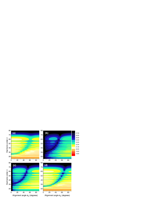
Figure 4: Contribution of different processes to the high-harmonic spectra, as functions of the alignment angle $\theta_{L}$, for the same field parameters in the previous figure, taking into account the degeneracy of the $1\pi_{u}$ orbitals in a three-dimensional scenario, and non-resolved angle $\phi_{p}$. The dipole matrix elements have been computed using a gaussian basis set and GAMESS-UK GAMESS . In this case, $E_{3\sigma_{g}}=0.63485797$ a.u, $E_{1\pi_{u}}=0.65087981$ a.u. and $R=2.068$ a.u. Panel (a): all processes,i.e., the full sum in Eq. 38; panel (b): processes incorporating the $1\pi_{u}$ orbitals only, i.e., $|M_{22}+M_{23}+M_{32}+M_{33}|^{2}$ in 38; panel (c): processes in which the electron starts at any orbital and recombines with the $1\pi_{u}$ orbitals, i.e.,$|M_{22}+M_{23}+M_{32}+M_{33}+M_{21}+M_{31}|^{2}$; panel (d): processes in which the electron recombines with the $3\sigma_{g}$ orbital, i.e., $|M_{11}+M_{12}+M_{13}|^{2}$.

In order to investigate this fact, we computed the high-order harmonic spectrum taking into account only the latter contributions. Such results are displayed in Fig. 4.(b). Qualitatively, the spectrum obtained in this way is in perfect agreement with those displayed in Fig. 2, which have been computed using $1\pi_{ux}$ only, or with that shown in Fig. 3.(b), which incorporates the processes in which the electron recombines at $1\pi_{ux}$ in a two-dimensional scenario. In fact, all such spectra exhibit a minimum above $\Omega=31\omega$ for $\theta_{p}$ in the vicinity of zero, which moves towards the cutoff for $\theta_{L}=45^{\circ}$. The harmonic yield in Fig. 4.(b), especially in the region of small alignment angles, is up to the three orders of magnitude weaker than the full spectrum. This huge discrepancy, however, would not cause any blurring in the full spectrum.

Potentially, the blurring may also be caused by the processes in which the electron is released from the $3\sigma_{g}$ orbital and recombines with any of the $1\pi_{u}$ orbitals. In this latter case, a minimum near $\Omega=31\omega$ for $\theta_{L}$ in the vicinity of zero would also be present. Therefore, such processes must be incorporated. In Fig. 4.(c), we consider the contributions from all possible processes finishing at the $1\pi_{u}$ orbitals, regardless of where the electron left from. As expected, there is a substantial increase in the yield for small angles, in comparison to Fig. 4.(b).

Such increase is however not sufficient to match the contributions from the $3\sigma_{g}$ states to the full spectrum. In Fig. 4.(d), we show that, for small alignment angles, the processes for which the electron recombines with the $3\sigma_{g}$ state dominate. In fact, for $0<\theta_{L}<45^{\circ}$ the yield in Fig. 4.(d) is roughly one order of magnitude larger than that displayed in Fig. 4.(c). This is not obvious, as there are twice as many more processes contributing to the yield in this latter case, namely six against three. A direct comparison of Figs. 4.(a) and  4.(d) also shows the above-mentioned dominance for small angles. For larger angles, the contributions from the $1\pi_{u}$ orbitals start to play a more significant role and there is an increase in the blurring. In all cases for which the electron only starts from or recombines with the $1\pi_{u}$ orbitals [Figs. 4.(b) and 4.(c)], there is a strong suppression of the yield for parallel alignment. This is due to the fact that the nodal plane along the molecular axis coincides with the laser-polarization axis in this case.

IV Conclusions

We considered the influence of two closely lying molecular orbitals on the high-order harmonic spectrum from $N_{2}$: the $1\pi_{u}$ and $3\sigma_{g}$ orbitals. We employed a very simple model, in which the strong-field approximation has been modified in order to incorporate the situations in which an electron leaves from the $3\sigma_{g}$ orbital and recombines with $1\pi_{u}$ and vice-versa. We have also included the degeneracy of the $1\pi_{u}$ orbital. We made a detailed assessment of the contributions of all possible processes to the high-order harmonic spectra.

The main conclusion to be drawn from this work is that the shape and the two-center interference patterns observed for the high-order harmonic spectra from $N_{2}$ are mainly determined by the $3\sigma_{g}$ orbital, even though the $1\pi_{u}$ orbitals are energetically very close. The main effect of the latter orbitals is to introduce some blurring in the interference minimum determined by $3\sigma_{g}$.

Physically, this is due to the particular geometry of the $1\pi_{u}$ orbitals. Indeed, for small alignment angles $\theta_{L}$, these orbitals exhibit a nodal plane close to the polarization axis, so that tunneling and recombination are strongly suppressed. Hence, in this region, the high-order harmonic spectra are mainly dominated by the $3\sigma_{g}$ orbital. We have verified that this dominance extends up to approximately $\theta_{L}=45^{\circ}$. For the parameters considered in this paper, the two-center minimum occurs within this region, so that it is mainly determined by the $3\sigma_{g}$ state.

Furthermore, due to their nontrivial dependence on the azimuthal angle, the $1\pi_{u}$ orbitals carry less weight when this parameter is integrated over. Interestingly, even if a three-dimensional computation is carried out and the degeneracy of the $1\pi_{u}$ orbitals is considered, this angular dependence outweighs the fact that there are more processes in which the electron recombines with one of the $1\pi_{u}$ orbitals.

We have also shown that, due to the above-mentioned non-trivial angular dependence, the influence of such orbitals is over-estimated if the dynamics of the problem is reduced to the $p_{x}p_{z}$ plane, i.e., if the azimuthal angle $\phi_{p}$ is chosen to be vanishing. Such an approximation has been extensively used in the literature (see, e.g., DM2009 in with HHG from the $\pi_{g}$ orbital of the $O_{2}$ molecule has been computed). This is not an obvious result, as two-dimensional models do not consider the degeneracy of the $1\pi_{u}$ orbital.

Finally, it is worth mentioning that the findings of this paper agree qualitatively with recent results obtained employing more sophisticated methods, such as Dyson orbitals and many-body perturbation theory Multielectron . Therein, it has been shown that many-electron effects did not play a significant role in the bound-state reconstruction of $N_{2}$, and that the information retrieved from the spectra was mostly related to the $3\sigma_{g}$ orbital.

It may, however, be possible to identify the influence of the $1\pi_{u}$ orbitals by looking at effects for perpendicular-aligned molecules, or relatively large alignment angles. In this case, the contributions from $3\sigma_{g}$ to the high-order harmonic spectrum are not expected to obfuscate those from $1\pi_{u}$. In fact, recently, the influence of the latter orbitals on the HHG spectrum of $N_{2}$ has been identified experimentally for perpendicular-aligned molecules, in form of a maximum at the rotational half-revival McFar2008 .

- (1) J. Itatani, J. Levesque, D. Zeidler, H. Niikura, H. Pépin, J. C. Kieffer, P. B. Corkum and D. M. Villeneuve, Nature 432, 867 (2004); W. Boutu, S. Haessler, H. Merdji, P. Breger, G. Waters, M. Stankiewicz, L. J. Frasinski, R. Taieb, J. Caillat, A. Maquet, P. Monchicourt, B. Carré and P. Salières, Nature Physics 4, 545 (2008).
- (2) H. Niikura, F. Légaré, R. Hasbani, A. D. Bandrauk, M. Yu. Ivanov, D. M. Villeneuve and P. B. Corkum, Nature 417, 917 (2002); H. Niikura, F. Légaré, R. Hasbani, M. Yu. Ivanov, D. M. Villeneuve and P. B. Corkum, Nature 421, 826 (2003); S. Baker, J. S. Robinson, C. A. Haworth, H. Teng, R. A. Smith, C. C. Chirilă, M. Lein, J. W. G. Tisch, J. P. Marangos, Science 312, 424 (2006).
- (3) B. Shan, X. M. Tong, Z. Zhao, Z. Chang, and C. D. Lin, Phys. Rev. A 66, 061401(R) (2002); F. Grasbon, G. G. Paulus, S. L. Chin, H. Walther, J. Muth-Böhm, A. Becker and F. H. M. Faisal, Phys. Rev. A 63, 041402(R)(2001); C. Altucci, R. Velotta, J. P. Marangos, E. Heesel, E. Springate, M. Pascolini, L. Poletto, P. Villoresi, C. Vozzi, G. Sansone, M. Anscombe, J. P. Caumes, S. Stagira, and M. Nisoli, Phys. Rev. A 71, 013409 (2005); T. Kanai, S. Minemoto and H. Sakai, Nature 435, 470 (2005).
- (4) P. B. Corkum, Phys. Rev. Lett. 71, 1994 (1993); K. C. Kulander, K. J. Schafer, and J. L. Krause in: B. Piraux et al. eds., Proceedings of the SILAP conference, (Plenum, New York, 1993).
- (5) M. Lein, N. Hay, R. Velotta, J. P. Marangos, and P. L. Knight, Phys. Rev. Lett. 88, 183903 (2002); Phys. Rev. A 66, 023805 (2002); M. Spanner, O. Smirnova, P. B. Corkum and M. Y. Ivanov, J. Phys. B 37, L243 (2004).
- (6) R. Torres and J. P. Marangos, J. Mod. Opt. 54, 1883 (2007); M. Gühr, B. K. McFarland, J. P. Farrel and P. H. Bucksbaum, J. Phys. B 40, 3745 (2007).
- (7) See, e.g., C. B. Madsen and L.B. Madsen, Phys. Rev. A 74, 023403 (2006); C. B. Madsen, A. S. Mouritzen, T. K. Kjeldsen, L. B. Madsen, Phys. Rev. A 76, 035401 (2007).
- (8) S. Odžak and D. B. Milošević, Phys. Rev. A 79, 023414 (2009); J. Phys. B 42, 071001 (2009).
- (9) V. I. Usachenko, and S. I. Chu, Phys. Rev. A 71, 063410 (2005); Vladimir I. Usachenko, Phys. Rev. A 73, 047402 (2006); V. I. Usachenko, P. E. Pyak, and Shih-I Chu, Laser Phys. 16, 1326 (2006); Vladimir I. Usachenko, Pavel E. Pyak, and Vyacheslav V. Kim, Phys. Rev. A 79, 023415 (2009).
- (10) D. B. Milošević, Phys. Rev. A 74, 063404 (2006); M. Busuladžić, A. Gazibegović-Busuladžić,D. B. Milošević, and W. Becker, Phys. Rev. Lett. 100, 203003 (2008); Phys. Rev. A 78, 033412 (2008).
- (11) A. T. Le, R. R. Lucchese, S. Tonzani, T. Morishita, and C. D. Lin, Phys. Rev. A 80, 013401 (2009).
- (12) Brian K. McFarland, Joseph P. Farrell, Philip H. Bucksbaum, Markus Gühr, Science 322 (5905), 1194 (2008).
- (13) S. Patchkovskii, Z. Zhao, T. Brabec and D. M. Villeneuve, Phys. Rev. Lett. 97, 123003 (2006); S. Patchkovskii, Z. Zhao, T. Brabec, and D.M. Villeneuve, J. Chem. Phys. 126, 114306 (2007); O. Smirnova, S. Patchkovskii, Y. Mairesse, N. Dudovich, D. Villeneuve, P. Corkum, and M. Yu. Ivanov, Phys. Rev. Lett. 102, 063601 (2009).
- (14) C.B. Madsen and L.B. Madsen, Phys Rev. A 76, 043419 (2007).
- (15) C. C. Chirilă and M. Lein, Phys. Rev. A 73, 023410 (2006).
- (16) O. Smirnova, M. Spanner and M. Ivanov, J. Phys. B 39, S307 (2006).
- (17) C. C. Chirilă and M. Lein, J. Mod. Opt. 54, 1039 (2007); G. N. Gibson and J. Biegert, Phys. Rev. A 78, 033423 (2008).
- (18) C. Figueira de Morisson Faria, Phys. Rev. A 76, 043407 (2007).
- (19) O. Smirnova, M. Spanner and M. Ivanov, J. Mod. Opt. 54, 1019 (2007).
- (20) M. Lewenstein, Ph. Balcou, M. Yu. Ivanov, A. L’Huillier and P. B. Corkum, Phys. Rev. A 49, 2117 (1994);W. Becker, A. Lohr, M. Kleber, and M. Lewenstein, Phys. Rev. A 56, 645 (1997).
- (21) P. Salières, B. Carré, L. LeDéroff, F. Grasbon, G. G. Paulus, H. Walther, R. Kopold, W. Becker, D. B. Milošević, A. Sanpera and M. Lewenstein, Science 292, 902 (2001).
- (22) C. Figueira de Morisson Faria, H. Schomerus and W. Becker, Phys. Rev. A 66, 043413 (2002).
- (23) C. Figueira de Morisson Faria and M. Lewenstein, J. Phys. B 38, 3251 (2005).
- (24) P. E. Cade, K. D. Sales and A. C. Wahl, J. Chem. Phys. 44, 1973 (1966).
- (25) GAMESS-UK is a package of ab initio programs. See: ”http://www.cfs.dl.ac.uk/gamess-uk/index.shtml”, M.F. Guest, I. J. Bush, H.J.J. van Dam, P. Sherwood, J.M.H. Thomas, J.H. van Lenthe, R.W.A Havenith, J. Kendrick, Mol. Phys. 103, 719 (2005).