Numerical Solution of the Small Dispersion Limit of the Camassa-Holm and Whitham Equations and Multiscale Expansions

Abstract

The small dispersion limit of solutions to the Camassa-Holm (CH) equation is characterized by the appearance of a zone of rapid modulated oscillations. An asymptotic description of these oscillations is given, for short times, by the one-phase solution to the CH equation, where the branch points of the corresponding elliptic curve depend on the physical coordinates via the Whitham equations. We present a conjecture for the phase of the asymptotic solution. A numerical study of this limit for smooth hump-like initial data provides strong evidence for the validity of this conjecture. We present a quantitative numerical comparison between the CH and the asymptotic solution. The dependence on the small dispersion parameter $\epsilon$ is studied in the interior and at the boundaries of the Whitham zone. In the interior of the zone, the difference between CH and asymptotic solution is of the order $\epsilon$, at the trailing edge of the order $\sqrt{\epsilon}$ and at the leading edge of the order $\epsilon^{1/3}$. For the latter we present a multiscale expansion which describes the amplitude of the oscillations in terms of the Hastings-McLeod solution of the Painlevé II equation. We show numerically that this multiscale solution provides an enhanced asymptotic description near the leading edge.

1 Introduction

The Camassa-Holm (CH) equation

$$u_{t}+(3u+2\nu)u_{x}-\epsilon^{2}(u_{xxt}+2u_{x}u_{xx}+uu_{xxx})=0,\quad x\in\mathbb{R},\quad t>0,$$ (1)

was discovered by Camassa and Holm [5] as a model for unidirectional propagation of waves in shallow water, $u(x,t)$ representing the height of the free surface about a flat bottom, $\nu$ being a constant related to the critical shallow water speed and $\epsilon$ a constant proportional to the mean water depth [13]. Equation (1) had been previously found by Fokas and Fuchssteiner [15] using the method of recursion operators and shown to be a bi-hamiltonian equation with an infinite number of conserved functionals. It was also rediscovered by Dai [9] as a model for nonlinear waves in cylindrical hyperelastic rods, with $u(x,t)$ representing the radial stretch relative to a pre-stressed state. Equation (1) finally also arises in the study of the motion of a non-Newtonian fluid of second grade in the limit when the viscosity tends to zero [4]. A class of two–component generalizations of the CH equation has been recently obtained in [14].

The initial value problem for (1)

$$u(x,0)=u_{0}(x),\quad\quad x\in\mathbb{R},$$

presents interesting features: first for $\nu=0$ there may exist peakons, i.e., non–smooth solutions, second even for a smooth initial datum $u_{0}(x)$ the wave-breaking phenomenon may occur, that is the solution $u(x,t)$ remains bounded while its slope becomes unbounded in finite time. This phenomenon was first noticed for $\nu=0$ by Camassa and Holm [5] who showed that for smooth and odd initial datum $u_{0}(x)$ such that $u_{0}(x)>0$ for $x<0$ and $u_{0}^{\prime}(0)<0$, the slope $u_{x}(x,t)$ is driven to $-\infty$ in finite time. In the case $\nu=0$, under the hypothesis that

$$m_{0}(x):=u_{0}(x)-\epsilon^{2}\partial_{xx}u_{0}(x)$$

is smooth and summable, McKean [23] proves that the wave-breaking phenomenon occurs if and only if some portion of the positive part of $m_{0}(x)$ lies to the left of some portion of the negative part of $m_{0}(x)$. The wave breaking phenomenon occurs also for $\nu\not=0$ and, in particular Constantin [6] shows that for initial data $u_{0}(x)$ in the Sobolev space $H^{s}(\mathbb{R})$, $s\geq 3$ there exists a unique solution to (1) $u\in{\cal C}^{0}([0,T[,H^{s}(\mathbb{R}))\cap{\cal C}^{1}([0,T[,H^{s-1}(\mathbb{R}))$ defined for some maximal time $T>0$; moreover $T<\infty$ if and only if $\liminf_{t\to T}\{\min_{x\in\mathbb{R}}u_{x}(x,t)\}=-\infty$, i.e., for $\nu\not=0$, singularities in the solution may arise only in the form of wave breaking.

In this manuscript we are interested in studying the behaviour of the solution $u(x,t,\epsilon)$ of the Cauchy problem of the CH equation as $\epsilon\rightarrow 0$ for smooth initial data for which breaking does not occur. To this end, we suppose that $u_{0}(x)$ is in the Schwartz class, has a single negative hump and satisfies the following non–breaking condition

$$m_{0}(x)+\nu>0,\quad x\in\mathbb{R}.$$ (2)

In this case for any $t>0$, $m(x,t;\epsilon)=u(x,t)-\epsilon^{2}\partial_{xx}u(x,t)$ is in the Schwartz class and $m(x,t;\epsilon)+\nu>0$ [7].

For initial data in this class and $\epsilon\ll 1$, Grava and Klein [17] show that the numerical solution $u(x,t,\epsilon)$ of (1) develops a zone of fast oscillations, as for the small dispersion limit of the Korteweg-de Vries (KdV) equation, see Fig. 1.

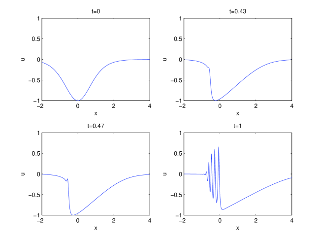
Fig. 1: Solution to the CH equation for $u_{0}=-\mbox{sech}^{2}x$, $\nu=1.2$ and $\epsilon=10^{-1.5}$ for several values of $t$.

In this paper, following the works of Gurevich and Pitaevskii [20], Lax and Levermore [25], Deift, Venakides and Zhou [10], we claim and give numerical support for our claim that the description of the small dispersion limit of the CH equation follows 1)-3) below:

1) For $0\leq t<t_{c}$, where $t_{c}$ is a critical time, the solution $u(x,t,\epsilon)$ of the CH Cauchy problem is approximated as $\epsilon\rightarrow 0$, by $u(x,t)$ which solves the Hopf equation

$$u_{t}+(3u+2\nu)u_{x}=0.$$ (3)

Here $t_{c}$ is the time when the first point of gradient catastrophe appears in the solution to the Hopf equation

$$u(x,t)=u_{0}(\xi),\quad\quad x=(3u_{0}(\xi)+2\nu)t+\xi,$$

and it is given by the relation

$$t_{c}=\frac{1}{\max_{\xi\in{\mathbb{R}}}[-3u^{\prime}_{0}(\xi)]}.$$

2) There exists $T>t_{c}$ such that for $t_{c}<t<T$, the solution of the CH equation is characterized by the appearance of an interval of rapid oscillations. If $f^{\prime\prime\prime}_{-}(u)<0$ where $f_{-}$ is the inverse of the decreasing part of the initial datum $u_{0}(x)$ and $u_{c}$ is the critical point, these oscillations are described in the following way. As $\epsilon\rightarrow 0$, the interval of the oscillatory zone is given by $[x^{-}(t),x^{+}(t)]$ where $x^{\pm}(t)$ are determined from the initial datum and satisfy the condition $x^{-}(t_{c})=x^{+}(t_{c})=x_{c}$, with $x_{c}$ the coordinate of the point of the gradient catastrophe of the Hopf solution. In the (x,t) plane $x^{\pm}(t)$ describe a cusp-shape region. Outside the interval $[x^{-}(t),x^{+}(t)]$ the leading order asymptotics is given by the solution of the Hopf equation. Inside the interval $(x^{-}(t),x^{+}(t))$ we claim that the solution $u(x,t,\epsilon)$ is approximately described, for small $\epsilon$ by the one–phase solution of CH which may be expressed in implicit form in terms of elliptic functions as

$$\left\{\begin{split}\displaystyle u(x,t,\epsilon)&\simeq\beta_{1}+\beta_{2}+\beta_{3}+2\nu-2(\beta_{3}+\nu)\frac{\Lambda(s,\rho)}{K(s)}+\frac{2}{I_{0}}\frac{d}{dz}\log\frac{\vartheta_{3}(z-p,\tau)}{\vartheta_{3}(z+p,\tau)},\\ \displaystyle\zeta&=\frac{k}{\epsilon}\left(x-(\beta_{1}+\beta_{2}+\beta_{3}+2\nu)t-q\right)=2\pi z-k\log\frac{\vartheta_{3}(z-p,\tau)}{\vartheta_{3}(z+p,\tau)},\end{split}\right.$$ (4)

with $\beta_{1}>\beta_{2}>\beta_{3}>-\nu$, $K(s)$ and $\Lambda(s,\rho)$ the complete Jacobi elliptic integrals of the first and third kind of modulus $s$, respectively, where

$$s^{2}=\frac{(\beta_{1}+\nu)(\beta_{2}-\beta_{3})}{(\beta_{2}+\nu)(\beta_{1}-\beta_{3})},\quad\quad\rho=\frac{\beta_{2}-\beta_{3}}{\beta_{2}+\nu}.$$ (5)

The quantities $I_{0}$, $p$ and the wave-number $k$ are Abelian integrals defined respectively in (10), (15) and (17), the phase shift $q(\boldsymbol{\beta})$ is defined in (24). $\vartheta_{3}(z,\tau)$ is the third Jacobi theta function of modulus $\tau=iK(\sqrt{1-s^{2}})/K(s)$ (see [32] and (14)).

For constant values of the $\beta_{i}$, (4) is an exact solution to CH in implicit form (see [2] and section 2). Moreover, for $-\nu<\beta_{3}<\beta_{2}<\beta_{1}$, such solution is real–periodic and analytic in $\zeta$, so it is appropriate to call it the one–phase solution. However, unlike the KdV case, it cannot be extended to meromorphic function on the $\zeta$ complex plane. Indeed, the r.h.s of the first equation in (4) is an elliptic function in $z$, while $\zeta=\zeta(z)$ is real analytic and invertible for real $z$, but not meromorphic in $\mathbb{C}$.

In the description of the leading order asymptotics of $u(x,t,\epsilon)$, as $\epsilon\to 0$, the quantities $\beta_{i}$ depend on $x,t$ and evolve according to the CH modulation equations which were derived in [1] for the one–phase periodic solution. In terms of the Riemann invariants $\beta_{3}<\beta_{2}<\beta_{1}$ they take the form

$${\partial_{t}}\beta_{i}+C_{i}(\boldsymbol{\beta}){\partial_{x}}\beta_{i}=0,\quad\quad C_{i}(\boldsymbol{\beta})=\frac{\partial_{\beta_{i}}\omega(\boldsymbol{\beta})}{\partial_{\beta_{i}}k(\boldsymbol{\beta})},\;\;i=1,2,3,$$ (6)

with $\boldsymbol{\beta}=(\beta_{1},\beta_{2},\beta_{3})$ and $\omega=(\beta_{1}+\beta_{2}+\beta_{3}+2\nu)k$. Unlike the KdV case, the Whitham equations for CH are not strictly hyperbolic and this fact gives some technical difficulties in their numerical and analytical treatment.

3) Near the left boundary of the cusp-shape region, in the double–scaling limit $x\rightarrow x^{-}(t)$ and $\epsilon\rightarrow 0$, in such a way that

$$(x-x^{-}(t))\epsilon^{-2/3}$$

remains finite, the asymptotic solution of the CH equation is given by

$$u(x,t,\epsilon)=u(x^{-}(t),t)+\epsilon^{\frac{1}{3}}a(x,t)\cos(\psi(x,t,\epsilon)/\epsilon)+O(\epsilon^{\frac{2}{3}}),$$

where $u(x,t)$ is the solution of the Hopf equation (3), the phase $\psi$ is given in (46) and the function $a(x,t,\epsilon)$ is, up to shifts and rescalings, the Hastings-Mcleod solution to the Painlevé-II equation [21]

$$A_{zz}=zA+2A^{3},\quad A,z\in\mathbb{C},$$

determined uniquely by the boundary conditions

$$A(z)\approx Ai(z)\quad(z\to+\infty),\quad\quad A(z)\approx\sqrt{-z/2}\quad(z\to-\infty)$$

with $Ai(z)$ the Airy function. Such a solution is real and pole free for real values of $z$.

We verify numerically the validity of the above asymptotic expansions 1), 2) and 3) for the initial datum $u_{0}(x)=-1/\cosh^{2}x$ and different values of $\nu$, see for instance Fig. 2.
Remark. The asymptotic description of $u(x,t,\epsilon)$ as $\epsilon\rightarrow 0$ near the critical time $t=t_{c}$ has been conjectured in [11] and studied numerically in [16]. The asymptotic description of $u(x,t,\epsilon)$ as $\epsilon\rightarrow 0$ at the right boundary of the cusp-shape region, namely near $x^{+}(t)$ has not yet been studied even for the KdV case.

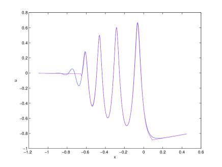
Fig. 2: Solution to the CH equation for the initial datum $u_{0}=-\mbox{sech}^{2}x$ and $\nu=1.2$ at $t=1$ in blue and the corresponding asymptotic solution via the Hopf equation and the one-phase CH solution solution.

The paper is organized as follows: In the next section we compute the one–phase solution to CH, in section 3 we obtain the small amplitude limit of the one–phase solution to the CH equation. In section 4 we perform a multiple scale analysis of the CH equations near the leading edge $x^{-}(t)$ of the oscillatory zone. In section 5 we present a numerical comparison of the small dispersion limit of the CH solution with the asymptotic formula (4). A quantitative numerical comparison of the CH solution and the multiscale solution is presented in section 6.

2 The one-phase solution to the Camassa–Holm equation

Let us look for a one–phase real–periodic travelling wave solution to (1) of the form

$$u(x,t)=(c-2\nu)-2\eta(\zeta),\quad\quad\zeta=\frac{kx-\omega t+\phi_{0}}{\epsilon},\quad\quad c=\frac{\omega}{k}$$

where $k$ is the wave number, $\omega$ the frequency and $\phi_{0}$ is a phase to be determined from the initial conditions. When we plug $\eta(\zeta)$ into the CH equation (1), after integration we get

$$k^{2}(\eta+\nu)\eta_{\zeta}^{2}-\eta^{3}+(c-2\nu)\eta^{2}-2B\eta+2A=0,$$ (7)

where $A$ and $B$ are constants of integration. The CH one-phase solution $u(x,t)=(c-2\nu)-2\eta(\zeta)$ is then obtained by inverting the differential of the third kind

$$\zeta=k\int_{\eta_{0}}^{\eta}\displaystyle\frac{(\xi+\nu)d\xi}{\sqrt{((\xi+\nu)(\xi^{3}+(2\nu-c)\xi^{2}+2B\xi-2A)}}=k\int_{\eta_{0}}^{\eta}\frac{(\xi+\nu)d\xi}{\sqrt{(\xi+\nu)\prod_{i=1}^{3}(\xi-\beta_{i})}},$$ (8)

where $\beta_{1}+\beta_{2}+\beta_{3}=c-2\nu$. Let $-\nu<\beta_{3}<\beta_{2}<\beta_{1}$, so that $\eta(\zeta)$ is real periodic in the interval $[\beta_{3},\beta_{2}]$. Since $\displaystyle\frac{d\zeta}{d\eta}$ has constant sign for $\eta\in[\beta_{3},\beta_{2}]$, by a standard argument, the (real) inverse function $\eta(\zeta)$ exists and is monotone in $\zeta\in[0,Z]$, where $Z$ is the half period of the travelling wave solution. To invert (8) and obtain $\eta=\eta(\zeta)$ let us introduce the elliptic curve

$${\mathcal{E}}:\;\{w^{2}=R(\xi)=(\xi+\nu)\prod_{i=1}^{3}(\xi-\beta_{i})\},$$ (9)

with homology basis of cycles $a,b$ as in the figure below and let

Fig. 3: The homology basis

$${\phi}=\frac{d\xi}{I_{0}w},\quad I_{0}=\oint_{a}\frac{d\xi}{w}=\frac{4K(s)}{\sqrt{(\beta_{2}+\nu)(\beta_{1}-\beta_{3})}},$$ (10)

be the normalized holomorphic differential on ${\mathcal{E}}$, with $K(s)$ the complete Jacobi elliptic integral of modulus $s$

$$s^{2}=\frac{(\beta_{1}+\nu)(\beta_{2}-\beta_{3})}{(\beta_{2}+\nu)(\beta_{1}-\beta_{3})}.$$ (11)

Then inversion of the normalized holomorphic differential

$$z=\int_{-\nu}^{\eta}\phi$$

is given by the Jacobi theorem [12] and takes the form

$$\eta(z)=\oint_{a}\xi\phi-\dfrac{1}{I_{0}}\dfrac{d}{dz}\log\dfrac{\vartheta_{3}(z-p_{0}+\frac{\tau}{2}+\frac{1}{2})}{\vartheta_{3}(z+p_{0}+\frac{\tau}{2}+\frac{1}{2})},$$ (12)

where

$$\oint_{a}\xi\phi=-\nu+(\nu+\beta_{3})\frac{\Lambda(s,\rho)}{K(s)},$$

$$\Lambda(s,\rho)=\int_{0}^{1}\frac{dz}{(1-\rho z^{2})\sqrt{(1-z^{2})(1-s^{2}z^{2})}},\quad\quad\rho=\frac{\beta_{2}-\beta_{3}}{\beta_{2}+\nu},$$ (13)

$\vartheta_{3}(z)$ is the third Jacobi-theta function defined by the Fourier series

$$\vartheta_{3}(z,\tau)=\sum_{n=-\infty}^{+\infty}\exp\left[i\pi n^{2}\tau+2\pi inz\right],\quad\quad\tau=i\frac{K^{\prime}(s)}{K(s)},$$ (14)

$K^{\prime}(s)=K(\sqrt{1-s^{2}})$ and $p_{0}$ is defined by

$$p_{0}=\int_{-\nu}^{\infty^{+}}\phi=\frac{1}{2}+p,\quad\quad p=\int_{\beta_{1}}^{\infty^{+}}\phi=\frac{1}{2K(s)}\int_{0}^{\sqrt{\frac{\beta_{2}+\nu}{\beta_{1}+\nu}}}\frac{dz}{\sqrt{(1-z^{2})(1-s^{2}z^{2})}}.$$ (15)

The function $\eta(z)$ is an elliptic function in $z$ with periods $1$ and $\displaystyle\tau$ and it is real periodic in $z$ along the complex line $z=\tau/2+z^{\prime}$, $z^{\prime}\in\mathbb{R}$.

Finally, inserting (12) into (8), we get

$$\zeta=kI_{0}\int^{z+\tau/2}_{\tau/2}(\eta+\nu)dz=kI_{0}(\nu+\beta_{3})\frac{\Lambda(s,\rho)}{K(s)}z-k\log\frac{\vartheta_{3}(z-p,\tau)}{\vartheta_{3}(z+p,\tau)}.$$ (16)

Equations (12) and (16) give the one–phase solution $u(\zeta)$ in implicit form. The real half period, $Z$, of $u(\zeta)$ is

$$Z=kI_{0}\int^{(\tau+1)/2}_{\tau/2}(\eta(z)+\nu)dz.$$ (17)

Normalizing the half period $Z$ to $\pi$, from (17) we obtain the wave number and the frequency

$$\begin{split}k&=2\pi\left(\oint_{a}\displaystyle\frac{(\xi+\nu)d\lambda}{\sqrt{R(\xi)}}\right)^{-1}=\frac{\pi\sqrt{(\beta_{2}+\nu)(\beta_{1}-\beta_{3})}}{2(\beta_{3}+\nu)\Lambda(s,\rho)},\\ \omega&=(2\nu+\beta_{1}+\beta_{2}+\beta_{3})k.\end{split}$$ (18)

Summarizing, the one–phase real nonsingular solution to the CH equation takes the form

$$\left\{\begin{array}[]{l}\displaystyle u(x,t,\epsilon)=\beta_{1}+\beta_{2}+\beta_{3}+2\nu-2(\beta_{3}+\nu)\frac{\Lambda(s,\rho)}{K(s)}+\frac{2}{I_{0}}\frac{d}{dz}\log\frac{\vartheta_{3}(z-p,\tau)}{\vartheta_{3}(z+p,\tau)},\\ \displaystyle\frac{1}{\epsilon}\left(x-(\beta_{1}+\beta_{2}+\beta_{3}+2\nu)t-q\right)=\frac{2\pi z}{k}-\log\frac{\vartheta_{3}(z-p,\tau)}{\vartheta_{3}(z+p,\tau)}.\end{array}\right.$$ (19)

Observe from the above formula that $u(x,t,\epsilon)$ is not a meromorphic function of $x$ and $t$. An alternative method to obtain $u(x,t,\epsilon)$ is discussed in [3] where the solution is expressed in terms of conveniently generalized theta-functions in two variables, which are constrained to the generalized theta-divisor of a 2–dimensional generalized Jacobian.

The envelope of the oscillations is obtained by the maximum and minimum values of the theta function and gives

$$\begin{split}u_{max}&=\beta_{1}+\beta_{2}+\beta_{3}+2\nu-2(\beta_{3}+\nu)\frac{\Lambda(s,\rho)}{K(s)}+\frac{4}{I_{0}}\frac{\vartheta^{\prime}_{3}(p+\frac{1}{2})}{\vartheta_{3}(p+\frac{1}{2})},\\ u_{min}&=\beta_{1}+\beta_{2}+\beta_{3}+2\nu-2(\beta_{3}+\nu)\frac{\Lambda(s,\rho)}{K(s)}+\frac{4}{I_{0}}\frac{\vartheta^{\prime}_{3}(p)}{\vartheta_{3}(p)}.\end{split}$$

3 Small amplitude limit of the one-phase solution

We analyze the one-phase solution (19) near the leading edge $x^{-}(t)$, namely when the oscillations go to zero. For this purpose we need to study the CH modulation equations more in detail.

3.1 Camassa-Holm modulation equations

In [1], Abenda and Grava constructed the one-phase CH modulation equations and showed that $\beta_{i}$, $i=1,2,3$ are the Riemann invariants. The CH modulation equations take the Riemann invariant form

$$\partial_{t}\beta_{i}+C_{i}({\boldsymbol{\beta}})\partial_{x}\beta_{i}=0,\quad\quad i=1,\dots,3,$$ (20)

where the speeds $C_{i}(\boldsymbol{\beta})$ in (6) are explicitly given by the formula [1]

$$\begin{split}&C_{1}(\boldsymbol{\beta})=\beta_{1}+\beta_{2}+\beta_{3}+2\nu+2\displaystyle\frac{(\beta_{3}+\nu)(\beta_{1}-\beta_{2})\Lambda(s,\rho)}{(\beta_{2}+\nu)E(s)},\\ &C_{2}(\boldsymbol{\beta})=\beta_{1}+\beta_{2}+\beta_{3}+2\nu+\displaystyle\frac{2(\beta_{2}-\beta_{3})\Lambda(s,\rho)}{K(s)-\displaystyle\frac{(\beta_{2}+\nu)(\beta_{1}-\beta_{3})}{(\beta_{3}+\nu)(\beta_{1}-\beta_{2})}E(s)}\\ &C_{3}(\boldsymbol{\beta})=\beta_{1}+\beta_{2}+\beta_{3}+2\nu+2\displaystyle\frac{(\beta_{3}+\nu)(\beta_{3}-\beta_{2})\Lambda(s,\rho)}{(\beta_{2}+\nu)[K(s)-E(s)]},\end{split}$$ (21)

with $\boldsymbol{\beta}=(\beta_{1},\beta_{2},\beta_{3})$, $K(s)$, $\Lambda(s,\rho)$ as before and $E(s)$ the complete elliptic integral of the second kind with modulus $s^{2}$. In the limit when two Riemann invariants coalesce, the modulation equations reduce to the Hopf equation

$$\partial_{t}u+(3u+2\nu)\partial_{x}u=0.$$

The CH modulation equations are integrable via the generalized hodograph transform introduced by Tsarev [30] ,

$$x=-C_{i}(\boldsymbol{\beta})\,t+w_{i}(\boldsymbol{\beta})\,\quad i=1,2,3\,,$$ (22)

which gives the solution of (20) in implicit form. The formula of the $w_{i}(\boldsymbol{\beta})$ for the specific CH case, has been obtained in [1], [19]:

$$w_{i}(\boldsymbol{\beta})=q(\boldsymbol{\beta})+\left(C_{i}(\boldsymbol{\beta})-(\beta_{1}+\beta_{2}+\beta_{3}+2\nu)\right)\partial_{\beta_{i}}q(\boldsymbol{\beta}),\quad\quad i=1,2,3,$$ (23)

where the function $q=q(\boldsymbol{\beta})$ is given by

$$q(\beta_{1},\beta_{2},\beta_{3})=\frac{1}{2\sqrt{2}}\int_{-1}^{1}\int_{-1}^{1}d\mu d\lambda\frac{f_{-}\left(\frac{1+\mu}{2}\left(\frac{1+\lambda}{2}\beta_{3}+\frac{1-\lambda}{2}\beta_{2}\right)+\frac{1-\mu}{2}\beta_{1}\right)}{\sqrt{1-\mu}\sqrt{1-\lambda^{2}}},$$ (24)

with $f_{-}$ the inverse of the decreasing part of the initial datum $u_{0}(x)$. The above formula of $q$ is valid for $x<x_{M}(t)$ where $x_{M}(t)$ is the coordinate of the minimum value of the solution $u(x,t)$ of the Hopf equation. For $x>x_{M}(t)$ the corresponding formula for $q$ contains also the increasing part of the initial datum (see [28]). In [19] it is shown that if $f_{-}^{\prime\prime\prime}(u_{c})<0$, then the solution $\beta_{1}(t)>\beta_{2}(t)>\beta_{3}(t)$ of the system (23) exists for some time $t>t_{c}$.

In order to take the small amplitude limit of the solution (4), we rewrite the system (22) in the equivalent form [19]

$$\left\{\begin{array}[]{l}(C_{1}t+w_{1}-x)\alpha=0,\\ \\ C_{2}t+w_{2}-x=0,\\ \\ \displaystyle\frac{(C_{2}-C_{3})t+(w_{2}-w_{3})}{\beta_{2}-\beta_{3}}=0,\end{array}\right.$$ (25)

where

$$\alpha=\frac{(\beta_{2}+\nu)E(s)}{(\beta_{1}-\beta_{2})(\beta_{3}+\nu)\Lambda(\rho,s)}\left(\beta_{1}-\frac{\beta_{2}+\beta_{3}}{2}\right),$$ (26)

with $s$ and $\rho$ as in (5) and (13), and we perform the limit $\delta\to 0$, where

$$\beta_{2}=v+\delta,\quad\quad\beta_{3}=v-\delta,\quad\quad\beta_{1}=u.$$

Let

$$\begin{split}Q(u,v)&=q(u,v,v)=\frac{\sqrt{2}}{4}\int_{-1}^{1}\frac{d\mu}{\sqrt{1-\mu}}f_{-}\left(\frac{1+\mu}{2}v+\frac{1-\mu}{2}u\right),\\ \Phi(u,v)&=\partial_{u}Q(u,v)+\partial_{v}Q(u,v)=\frac{\sqrt{2}}{4}\int_{-1}^{1}\frac{d\mu}{\sqrt{1-\mu}}f_{-}^{\prime}\left(\frac{1+\mu}{2}v+\frac{1-\mu}{2}u\right),\end{split}$$ (27)

then the following identities hold

$$\begin{split}f_{-}(u)&=Q(u,v)+2(u-v)\partial_{u}Q(u,v),\\ \partial_{uv}Q(u,v)&=\frac{2\partial_{u}Q(u,v)-\partial_{v}Q(u,v)}{2(u-v)},\\ \partial_{uvv}Q(u,v)&=\frac{4\partial_{uv}Q(u,v)-\partial_{vv}Q(u,v)}{2(u-v)},\end{split}$$ (28)

Substituting (27), (28) and the expansion of the elliptic integrals $E(s)$, $K(s)$ and $\Lambda(s,\rho)$ as $s,\rho\rightarrow 0$ [19] into (25), we arrive to the system

$$\begin{split}x=&(3u+2\nu)t+f_{-}(u)-\frac{\delta^{2}}{2}\frac{(3t+\Phi(u,v))(2v+u+3\nu)}{(u-v)^{2}}+O(\delta^{3}),\\ \displaystyle x=&(3u+2\nu)t+f_{-}(u)-2\frac{u-v}{u+\nu}\left(t(u+2v+3\nu)+\Phi(u,v)(v+\nu)+\partial_{u}Q(u,v)(u-v)\right)\\ &+\delta\left(\frac{(2v-u+\nu)(3t+\Phi(u,v))-2(u-v)(v+\nu)\partial_{v}\Phi(u,v)}{2(u+\nu)}\right)-\delta^{2}\left(\partial_{vv}\Phi(u,v)\cdot\right.\\ &\left.\cdot\frac{(u-v)(v+\nu)}{2(u+\nu)}-\frac{8v^{2}-8uv+8v\nu-2u\nu+3\nu^{2}+3u^{2}}{8(u+\nu)(v+\nu)(u-v)}(3t+\Phi(u,v))\right)+O(\delta^{3}),\\ \displaystyle 0=&\frac{(2v-u+\nu)(3t+\Phi(u,v))-2(u-v)(v+\nu)\partial_{v}\Phi(u,v)}{2(u+\nu)}+O(\delta^{2}).\end{split}$$ (29)

From the above, we deduce that, in the limit $\delta\to 0$, the hodograph transform (22) reduces to the form

$$\left\{\begin{split}0&=(3u(t)+2\nu)t+f_{-}(u)-x,\\ 0&=(u-v)(t+\partial_{u}Q(u,v))+(v+\nu)(3t+\Phi(u,v)),\\ 0&=(u-2v-\nu)(\Phi(u,v)+3t)+2(v+\nu)(u-v)\partial_{v}\Phi(u,v).\end{split}\right.$$ (30)

The above system of equations enables one to determine $x$, $u$ and $v$ as functions of time. We denote this time dependence as $x=x^{-}(t)$, $v=v(t)$ and $u=u(t)$. Observe that $u(t)=u(x^{-}(t),t)$ where $u(x,t)$ is the solution of the Hopf equation. In what follows we will always denote by $u$ or $u(t)$ the solution of the Hopf equation $u(x,t)$ at the leading edge $x=x^{-}(t)$ while we will refer to the solution of the CH equation as $u(x,t,\epsilon)$. The derivatives with respect to time of these quantities are given by

$$\begin{split}x^{-}_{t}&=3u+2\nu+(3t+f^{\prime}(u))u_{t},\\ u_{t}&=-2\frac{(u-v)(u+2v+3\nu)}{(u+\nu)(3t+f^{\prime}_{-}(u))},\\ v_{t}&=-\frac{4(u-3\nu-4v)(v+\nu)(u-v)}{V},\end{split}$$ (31)

with

$$V=4(v+\nu)^{2}(u-v)^{2}\partial_{vv}\Phi(u,v)-(3t+\Phi(u,v))(8v\nu+3u^{2}-8uv-2u\nu+3\nu^{2}+8v^{2}).$$ (32)

We are interested in studying the behaviour of the one–phase solution (19) near the leading edge, namely when $0<x-x^{-}(t)\ll 1$. To this aim, we introduce two unknown functions of $x$ and $t$,

$$\delta=\delta(x-x^{-}(t)),\quad\quad\quad\Delta=\Delta(x-x^{-}(t)),$$

which tend to zero as $x\to x^{-}(t)$. We now derive the dependence of $\Delta$ as a function of $x-x^{-}(t)$. Let us fix

$$\beta_{2}=v+\delta,\quad\quad\beta_{3}=v-\delta,\quad\quad\beta_{1}=u+\Delta,\quad\quad\Delta\to 0.$$ (33)

For the first equation in (25) near $\delta=0$, we find

$$x=(3\beta_{1}+2\nu)t+f_{-}(\beta_{1})-\frac{\delta^{2}}{2}\frac{(3t+\Phi(\beta_{1},v))(2v+\beta_{1}+3\nu)}{(\beta_{1}-v)^{2}}+O(\delta^{3}).$$

We then substitute $\beta_{1}=u+\Delta$ in the above equation, we insert (27), (28) and (30) into it, and we get

$$x-x^{-}(t)\approx\Delta(f^{\prime}_{-}(u)+3t)-\frac{\delta^{2}}{4}\frac{(u+2v+3\nu)(x-x^{-}(t))}{(u-v)^{2}(v+\nu)},$$ (34)

so that

$$\Delta\approx\frac{x-x^{-}(t)}{3t+f^{\prime}_{-}(u)}.$$ (35)

Similarly, using the second equation in (25), we arrive at

$$x-x^{-}(t)\approx\delta^{2}c,\quad\quad c=-\frac{V}{8(u+\nu)(v+\nu)(u-v)}>0,$$ (36)

with $V$ defined in (32).

Theorem 1.

In the limit

$$\beta_{2}=v+\delta,\quad\quad\beta_{3}=v-\delta,\quad\quad\beta_{1}=u+\Delta,\quad\quad\delta,\Delta\to 0,$$

the one-phase solution of the CH equation, implicitly defined by (4), has the following trigonometric expansion

$$u(x,t,\epsilon)\approx u(t)+\frac{x-x^{-}(t)}{3t+f^{\prime}_{-}(u)}+2\delta\cos\left(\frac{\xi}{\epsilon}\right)-\frac{\delta^{2}}{2}\frac{u+\nu}{(u-v)(v+\nu)}\left(1-\cos\left(2\frac{\xi}{\epsilon}\right)\right),$$ (37)

with

$$\begin{split}&\xi=\xi_{0}+\xi_{1}+O((x-x_{-}(t))^{2}),\\ &\xi_{0}=-2\sqrt{(u-v)(v+\nu)}(\Phi(u,v)+3t)\quad\quad\xi_{1}=\sqrt{\frac{u-v}{v+\nu}}(x-x_{-}(t)).\end{split}$$ (38)

Proof: We first prove (38). Let $\zeta=\xi/\epsilon$ in (4), so that

$$\xi=k\left[x-(\beta_{1}+\beta_{2}+\beta_{3}+2\nu)t-q(\beta_{1},\beta_{2},\beta_{3})\right],$$

with $k$ as is (10), $q$ as in (24). In the limit $\delta,\Delta\to 0$, with $\beta_{2}=v+\delta$, $\beta_{3}=v-\delta$, $\beta_{1}=u+\Delta$, we get

$$\begin{split}\xi&=\sqrt{\frac{u-v}{v+\nu}}\left(1+\frac{\Delta}{2(u-v)}\right)\left(1-\frac{\delta^{2}}{16}\frac{(u+\nu)(3\nu+4v-u)}{(v+\nu)^{2}(u-v)^{2}}\right)\bigg{(}x-\\ &\left.-(u+2\nu+2v+\Delta)t-Q(u,v)-\Delta\partial_{u}Q(u,v)-\frac{\delta^{2}}{4}\partial_{vv}Q(u,v)\right)+O(\delta^{4}),\end{split}$$

where we use $\Delta=O(\delta^{2})$ to estimate the error in the formula above. Then, we insert the solution $x_{-}(t)$ of equations (30), we use (35) and (36) to estimate $\Delta$ and $\delta^{2}$ and we get

$$\xi=-2\sqrt{(u-v)(v+\nu)}(\Phi(u,v)+3t)+\sqrt{\frac{u-v}{v+\nu}}(x-x_{-}(t))+O((x-x_{-}(t))^{2}),$$

where $\Phi$ is defined in (27), which coincides with (38).

We now prove that in the limit $\delta\to 0$, $u(x,t,\epsilon)$, defined implicitly as a function of $\zeta$ in (4), has the following trigonometric series expansion

$$u(x,t,\epsilon)=\beta_{1}+2\delta\cos(\zeta)-\frac{\delta^{2}}{2}\frac{\beta_{1}+\nu}{(\beta_{1}-v)(v+\nu)}\left(1-\cos(2\zeta)\right)+O(\delta^{3}).$$ (39)

To this aim, we expand $u(x,t,\epsilon)$ and $\zeta$ defined in (4) in trigonometric series of $z$ and we compute $z$ as a function of $\zeta$.

We need the following series expansions for the Jacobi theta functions [32]

$$\begin{split}\displaystyle\log\left(\frac{\vartheta_{3}(z-p)}{\vartheta_{3}(z+p)}\right)&=4\sum_{n=1}^{+\infty}\frac{(-1)^{n+1}}{n}\frac{{\tt q}^{n}}{1-{\tt q}^{2n}}\sin(2n\pi z)\sin(2n\pi p),\\ \displaystyle\frac{\vartheta^{\prime}_{3}(z\pm p)}{\vartheta_{3}(z\pm p)}&=4\pi\sum_{n=1}^{+\infty}(-1)^{n}\frac{{\tt q}^{n}}{1-{\tt q}^{2n}}\sin(2n\pi(z\pm p)),\end{split}$$ (40)

where $p$ is as in (15) and

$${\tt q}=\exp\left(-\pi K^{\prime}(s)/K(s)\right)=\frac{(\beta_{1}+\nu)}{8(v+\nu)(\beta_{1}-v)}\delta+O(\delta^{3}).$$ (41)

Inserting the above expansion and

$$\begin{split}\sin(2\pi p)&=2\frac{\sqrt{(v+\nu)(\beta_{1}-v)}}{\beta_{1}+\nu}+O(\delta^{2}),\\ \sin(4\pi p)&=-4\frac{(2v+\nu-\beta_{1})\sqrt{(v+\nu)(\beta_{1}-v)}}{(\beta_{1}+\nu)^{2}}+O(\delta^{2}),\end{split}$$

into (40), we get

$$\begin{split}u(x,t,\epsilon)&=\beta_{1}+2\delta\cos(2\pi z)+\frac{\delta^{2}}{2}\frac{\beta_{1}-\nu-2v}{(v+\nu)(\beta_{1}-v)}\left(1-\cos(4\pi z)\right)+O(\delta^{3}),\\ \zeta&=2\pi z-\frac{\delta}{v+\nu}\sin(2\pi z)+O(\delta^{2})\end{split}$$

from which we find

$$2\pi z=\zeta+\frac{\sin(\zeta)}{v+\nu}\delta+O(\delta^{2}),$$

and the assertion easily follows. $\square\quad$

4 Painlevé equations at the leading edge

In this section we propose a multiscale description of the oscillatory behavior of the solution to the CH equation in the small dispersion limit ($\epsilon\to 0$) close to the leading edge $x_{-}(t)$ where $\beta_{2}=\beta_{3}=v$ and $\beta_{1}=u$. We follow closely the approach [18] for the corresponding KdV situation. The ansatz for the multiscale expansion to the CH solution close to the leading edge is inspired by the asymptotic solution in the Whitham zone discussed in the previous section. Numerically we find that the quantity $\delta$ in (37) is of the order $\epsilon^{1/3}$. This implies with (36) that $x-x_{-}(t)\approx\epsilon^{2/3}$ in the double scaling limit $\epsilon\to 0$ and $x\to x_{-}(t)$. We are thus led to introduce the rescaled coordinate $y$ near the leading edge,

$$y=\epsilon^{-2/3}(x-x_{-}(t)),$$ (42)

which transforms the CH equation (1) to the form

$$(3u+2\nu-x_{t}^{-})u_{y}+\epsilon^{2/3}(u_{t}-2u_{y}u_{yy}-(u-x^{-}_{t})u_{yyy})-\epsilon^{4/3}u_{yyt}=0,$$ (43)

where $x_{t}^{-}=\frac{d}{dt}x_{-}(t).$

Numerically the corrections to the Hopf solution near the leading edge are of order $\epsilon^{1/3}$ and thus we make as in [18] the ansatz

$$u(y,t,\epsilon)=U_{0}(y,t)+\epsilon^{1/3}U_{1}(y,t)+\epsilon^{2/3}U_{2}(y,t)+\epsilon U_{3}(y,t)+\dots,$$ (44)

where $U_{0}=u(t)$ is the solution of the Hopf equation at the leading edge. We assume that the terms $U_{k}$, $k\geq 1$ contain oscillatory terms of the order $1/\epsilon$ and take the form

$$\begin{split}U_{1}(y,t)&=a(y,t)\cos\left(\frac{\psi(y,t)}{\epsilon}\right),\\ U_{2}(y,t)&=b_{1}(y,t)+b_{2}(y,t)\cos\left(\frac{2\psi(y,t)}{\epsilon}\right),\\ U_{3}(y,t)&=c_{0}(y,t)+c_{1}(y,t)\cos\left(\frac{\psi(y,t)}{\epsilon}\right)+c_{2}(y,t)\sin\left(\frac{2\psi(y,t)}{\epsilon}\right)+\\ &+c_{3}(y,t)\cos\left(\frac{3\psi(y,t)}{\epsilon}\right),\end{split}$$ (45)

where

$$\psi(y,t)=\psi_{0}(y,t)+\epsilon^{1/3}\psi_{1}(y,t)+\epsilon^{2/3}\psi_{2}(y,t)+\epsilon\psi_{3}(y,t)+\dots.$$ (46)

Terms proportional to $\sin(\psi/\epsilon)$ in $U_{1}$ can be absorbed by a redefinition of $\psi$, the higher order terms are chosen to compensate terms of lower order appearing in the solution to CH due to the non-linearities. We immediately find $\partial_{y}\psi_{0}=0=\partial_{y}\psi_{1}$ from the terms of order $\epsilon^{-2}$ and $\epsilon^{-1}$. The term of order $\epsilon^{0}$ gives

$$\left(1+(\partial_{y}\psi_{2})^{2}\right)\partial_{t}\psi_{0}+\partial_{y}\psi_{2}\left(3u+2\nu-x^{-}_{t}\right)+\left(u(t)-x^{-}_{t}\right)(\partial_{y}\psi_{2})^{3}=0.$$ (47)

In particular, (47) is algebraic in $\partial_{y}\psi_{2}$ with coefficients depending on $t$ only, i.e., $\psi_{2}(y,t)=f_{2}(t)y+f_{1}(t)$, with $f_{1,2}(t)$ to be determined. At the order $\epsilon^{1/3}$, we get $\partial_{t}\psi_{1}=0$ and

$$a^{2}\left(1+f_{2}^{2}\right)^{2}=8b_{2}f_{2}^{2}\left(u+\nu\right),$$ (48)

$$f_{2}^{4}(x^{-}_{t}-u)+2f_{2}^{2}(x^{-}_{t}+\nu)+x^{-}_{t}-2\nu-3u=0.$$ (49)

At the order $\epsilon^{2/3}$, using (47) to (49), we find $\partial_{y}\psi_{3}=0$ and

$$c_{2}=\frac{a\partial_{y}a\left(f_{2}^{4}-1\right)}{4(u+\nu)f_{2}^{3}},\quad\quad c_{3}=\frac{a^{3}\left(3+7f_{2}^{2}\right)\left(1+f_{2}^{2}\right)^{3}}{256(u+\nu)^{2}f_{2}^{4}},$$ (50)

$$b_{1}=-\frac{1}{8}\frac{(a^{2}(3+f_{2}^{2})+4u_{t}y)(1+f_{2}^{2})^{2}}{f_{2}^{2}(3+f_{2}^{2})(u+\nu)}+g_{1}(t),$$ (51)

with $g_{1}(t)$ integration constant,

$$\begin{split}\partial_{yy}a&-\frac{\left(1+f_{2}^{2}\right)^{4}}{32(u+\nu)^{2}f_{2}^{2}}a^{3}+\frac{ay}{4}\frac{u_{t}\left(1+f_{2}^{2}\right)^{4}}{f_{2}^{2}(-3+f_{2}^{2})(u+\nu)^{2})}\\ &-\frac{a}{2}\frac{(1+f_{2}^{2})^{3}\partial_{t}\psi_{2}}{f_{2}(u+\nu)(-3+f_{2}^{2})}-\frac{g_{1}a}{2}\frac{(3+f_{2}^{2})(1+f_{2}^{2})^{2}}{(u+\nu)(-3+f_{2}^{2})}=0.\end{split}$$ (52)

We determine $\partial_{y}\psi_{2}$ inserting (31) inside (49), so that

$$\partial_{y}\psi_{2}^{2}=f_{2}^{2}\in\left\{\frac{u-v}{v+\nu},\frac{2v+u+3\nu}{u-\nu-2v}\right\},$$ (53)

where the sign in front of the square root has to be chosen in such a way that the r.h.s. is positive. Then comparing (53), (46), (38) and (42), we conclude that

$$\psi_{2}(y,t)=y\sqrt{\frac{u-v}{v+\nu}}.$$ (54)

Inserting (54) into (47), we find

$$\partial_{t}\psi_{0}(t)=-4\sqrt{\frac{v+\nu}{u-v}}\frac{(u-v)^{2}}{u+\nu}.$$ (55)

By comparison with (38), we observe that

$$-2\frac{d}{dt}\left(\sqrt{(u-v)(v+\nu)}(\Phi(u,v)+3t)\right)=-4\sqrt{\frac{v+\nu}{u-v}}\frac{(u-v)^{2}}{(u+\nu)}.$$

Then integrating the l.h.s.  of the above expression between $t_{c}$ and $t$ we arrive at (38), namely

$$\psi_{0}(t)=-2\sqrt{(u-v)(v+\nu)}(\Phi(u,v)+3t).$$ (56)

Moreover, consistency between (44) and (37) implies that

$$\delta=\frac{\epsilon^{1/3}a}{2},$$ (57)

from which we immediately verify that

$$\epsilon^{2/3}b_{2}=\frac{\delta^{2}}{2}\frac{u+\nu}{(u-v)(v+\nu)},$$

$$\epsilon^{2/3}b_{1}=\frac{x-x_{-}(t)}{3t+f^{\prime}(u)}-\frac{\delta^{2}}{2}\frac{u+\nu}{(u-v)(v+\nu)},$$

with $g_{1}(t)\equiv 0$ in (51).

Summarizing, we get

$$u(x,t,\epsilon)=u(t)+\epsilon^{1/3}a\cos\left(\frac{\psi}{\epsilon}\right)+\epsilon^{2/3}\left[\frac{a^{2}(u+\nu)(\cos(2\psi/\epsilon)-1)}{8(u-v)(v+\nu)}+\frac{y}{3t+f^{\prime}(u)}\right]+O(\epsilon),$$ (58)

where

$$\psi(y,t)=-2\sqrt{(u-v)(v+\nu)}(\Phi(u,v)+3t)+\epsilon^{2/3}y\sqrt{\frac{u-v}{v+\nu}}+O(\epsilon),$$ (59)

with $Phi(u,v)$ defined in (27) and $a$ satisfies the Painlevé-II equation

$$\partial_{yy}a-A_{1}ay-A_{2}a^{3}=0,$$ (60)

with

$$A_{1}=\frac{(u+\nu)^{3}v_{t}}{4(u-v)(v+\nu)^{3}(3\nu+4v-u)}\quad\quad A_{2}=\frac{(u+\nu)^{2}}{32(u-v)(v+\nu)^{3}}.$$ (61)

Using (31), we get

$$A_{1}=\frac{(u+\nu)^{3}}{V(v+\nu)^{2}}.$$

with $V$ defined in (32). Making the substitution $z=\alpha y$, $a=\beta A$ with

$$\alpha=\left(A_{1}\right)^{1/3},\quad\quad\beta=\frac{\alpha\sqrt{2}}{\sqrt{A_{2}}},$$

we arrive to the special Painlevé II equation in normal form

$$A_{zz}=zA+2A^{3}.$$ (62)

For $x-x_{-}(t)>0$, from the small amplitude limit of the one–phase solution to the CH equation we get

$$a=2\epsilon^{-1/3}\delta\approx 2\epsilon^{-1/3}\sqrt{\frac{x-x_{-}}{c}},$$

with $c$ defined in (36), so that in the limit $\epsilon\to 0+$ (equivalently $y\to+\infty$ or $z\to-\infty$), we have

$$A(z)\approx\sqrt{-z/2}.$$

If $x\ll x_{-}(t)$, the CH solution is approximately the solution to the Hopf equation so that $a(y)\approx 0$, for $y\to-\infty$ (equivalently $z\to+\infty$). Therefore we conclude that

$$\lim_{z\to+\infty}A(z)=0.$$

The solution to the Painlevé II equation satisfying such asymptotic condition exists and is unique and pole free on the real line according to Hastings and McLeod [21].

5 Numerical solution of CH and Whitham equations

In this section we will solve numerically the CH and the Whitham equations for initial data in the Schwartzian class of rapidly decreasing functions with a single negative hump. As a concrete example we will study the initial datum

$$u_{0}:=u(x,0)=-\mbox{sech}^{2}x.$$ (63)

For this initial datum the non–breaking condition (2) is satisfied if $\epsilon^{2}<(\nu-1)/2$.

5.1 Numerical solution of the CH equation

The resolution of the rapid modulated oscillations in the region of a dispersive shock is numerically demanding. The strong gradients in the oscillatory regions require efficient approximation schemes which do not introduce an artificial numerical dissipation into the system. We therefore use Fourier spectral methods which are known for their excellent approximation properties for smooth functions whilst minimizing the introduction of numerical viscosity. We restrict to initial data, where $u_{0}-\epsilon^{2}u_{0,xx}+\nu$ does not change sign, to ensure analyticity of the CH solutions. The Schwartzian solutions can be treated as effectively periodic if the computational domain is taken large enough that the solution is of the order of machine precision ($\approx 10^{-16}$ in Matlab) at the boundaries. We always choose the computational domain in this way to avoid Gibbs phenomena at the boundaries.

Even with spectral methods, a large number of Fourier modes is needed to resolve the rapid oscillations numerically. To obtain also a high resolution in time, we use high order finite difference methods, here a fourth order Runge-Kutta scheme. For stability reasons a sufficiently small time step has to be chosen. Unconditionally stable implicit schemes could be used instead, but these can be only of second order. Such approaches would be too inefficient for the precision requested. Notice that the terms with the highest derivative in CH (1) are not linear in contrast to the KdV equation (we choose the KdV equation in a way that it has the same dispersionless equation as (1), the term proportional to $\nu$ can be always eliminated here in contrast to CH by a Galilean transformation)

$$u_{t}+(3u+2\nu)u_{x}+\epsilon^{2}u_{xxx}=0.$$ (64)

For such equations efficient integration schemes are known. In [24] it was shown that exponential time differentiation (ETD) methods [8, 26] are the most efficient in the small dispersion limit of KdV. For CH such an approach is not possible due to the nonlinearity of the highest order derivatives. But we can use analytic knowledge of the solution: The dispersionless equation, the Hopf equation, will have a point of gradient catastrophe at the critical time $t_{c}$, for the example (63) $t_{c}=\sqrt{3}/4\approx 0.433$. For times $t\ll t_{c}$, the CH solution is very close to the Hopf solution with moderate gradients. In this case we can use a larger time step. For times close to the critical time and beyond (in our example $t>0.4$), we have to use considerably smaller time steps.

The main difference to the KdV equation is the non-locality of CH, which provides some filtering for the high frequencies: if we denote the Fourier transform of $u$ with respect to $x$ by $\hat{u}(k,t):=\int_{-\infty}^{\infty}u(x,t)e^{ikx}dx$, we get for (1) in Fourier space

$$\hat{u}_{t}=\frac{1}{1+\epsilon^{2}k^{2}}\left(\frac{3}{2}ik\widehat{u^{2}}+2\nu ik\hat{u}-\epsilon^{2}(2\widehat{u_{x}u_{xx}}+\widehat{uu_{xxx}})\right).$$

The term $1/(1+\epsilon^{2}k^{2})$ in the above equation is the reason why CH gives for large spatial frequencies a better approximation to one-dimensional wave phenomena than KdV with a term proportional to $k^{3}$ in Fourier space. Its effect in the present context is twofold: First it provides a high frequency filtering which allows in practice for larger time steps in the computation. Secondly it suppresses the rapid modulated oscillations in the shock region of the dispersionless equation. This can be seen in Fig. 4, where solutions to KdV and CH for the same initial data are shown.

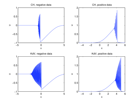
Fig. 4: Solution to the CH equation (1) and KdV equation (64) with $\nu=1.2$ for the initial data $u_{0}=-\mbox{sech}^{2}x$ on the left side and $u_{0}=\mbox{sech}^{2}x$ on the right side at $t=1$ for $\epsilon=10^{-2}$.

The KdV solutions always show much more oscillations than the CH solutions.

Notice that despite the lower number of oscillations in the CH solutions in Fig. 4, depending on the value of $\nu$ a higher number of Fourier modes is needed to resolve the oscillations. This is due to the fact that the CH solution is less smooth than the KdV solution and thus less localized in Fourier space, as can be seen in Fig. 5.

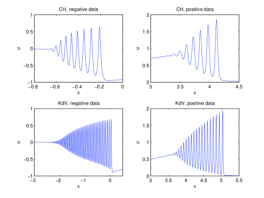
Fig. 5: Magnification of the oscillations in Fig. 4.

Therefore, to treat the same values of the small dispersion parameter $\epsilon$ for CH as for KdV, we need higher temporal and spatial resolution. It is thus computationally more demanding to obtain the same number of oscillations in CH solutions as in KdV solutions, the latter being important to obtain a valid statistics for the scaling studied below.

The quality of the numerics is controlled via energy conservation for CH,

$$E\sim 2\nu u^{2}+\epsilon^{2}uu_{x}^{2}+u^{3}.$$

The numerically computed energy will depend on time due to numerical errors. As was discussed in [24], energy conservation can thus be used to check numerical accuracy. In practice energy conservation overestimates numerical precision by 1-2 order of magnitude. We typically solve the CH equation with a relative numerical error $\Delta E/E=10^{-6}$. This ensures that the difference between the numerical and the asymptotic CH solution, which is typically of the order of $\epsilon$ or larger, is entirely due to the asymptotic description.

5.2 Numerical solution to the Whitham equations

The Whitham equations (6) have a similar form as the respective equations for KdV. We use the same procedure to solve them numerically: we first solve the equations at the edges of the Whitham zone and then at intermediate points. For details the reader is referred to [18]. Typical solutions for the Whitham equations can be seen in Fig. 6. In the shown example, the quantity $\beta_{3}$ crosses the hump at $-1$.

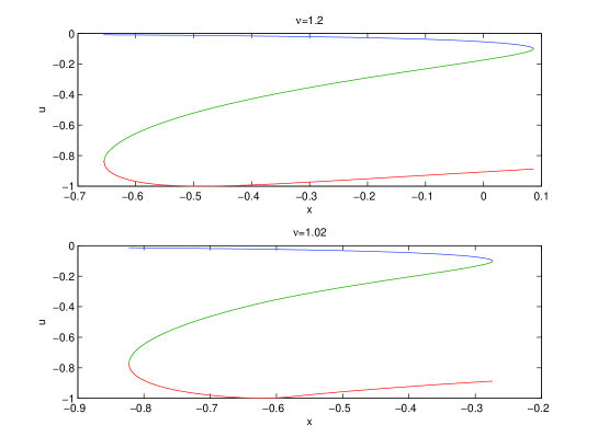
Fig. 6: Solutions $\beta_{i}$, $i=1,2,3$ to the Whitham equations (6) for $u_{0(x)}=-\mbox{sech}^{2}x$ and $t=1$ for two values of $\nu$.

In contrast to KdV, the system (6) is not strictly hyperbolic, i.e., the speeds $C_{i}$, $i=1,2,3$, in (21) do not satisfy for all $x$ and $t>t_{c}$ the relation $C_{1}>C_{2}>C_{3}$. In fact the lines $C_{i}(x)$ can cross for a given time for $\nu\sim 1$ as can be seen in Fig. 7.

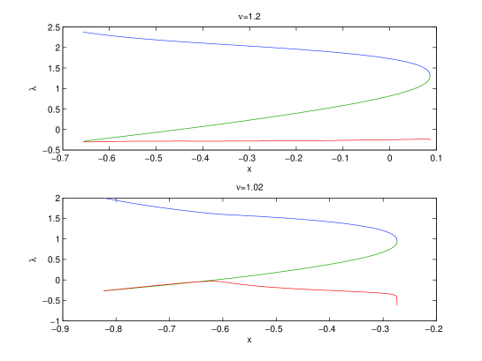
Fig. 7: The speeds $C_{i}$, $i=1,2,3$ (21) for $u_{0}(x)=-\mbox{sech}^{2}x$ and $t=1$ for two values of $\nu$.

For $\nu=1.02$ the speeds $C_{2}$ and $C_{3}$ intersect in the shown example in the interior of the Whitham zone as can be seen in more detail in Fig. 8.

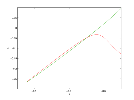
Fig. 8: Magnification of the lines in the lower figure of Fig. 7 close to the crossing of the lines.

This behavior of the speeds has no influence on the numerical solubility of the Whitham equations. It also does not influence the quality of the asymptotic solution in these cases as can be seen in Fig. 9.

5.3 Quantitative comparison of the CH solution and the asymptotic solution

The asymptotic description of the small dispersion limit of the CH equation is as follows: for times $t<t_{c}$, the Hopf solution for the same initial datum provides an asymptotic description. For $t>t_{c}$, the Whitham zone opens. Outside this zone, the Hopf solution again serves as an asymptotic solution. In the interior the one-phase solution to the CH equation describes the oscillatory behavior. It is given on an elliptic curve with branch points being solutions of the Whitham equations.

Below we will study the validity of this asymptotic description in various regions of the ($x,t$)-plane. To study the $\epsilon$ dependence of a certain quantity $A$, we perform a linear regression analysis for the dependence of the logarithms, $\ln A=a\ln\epsilon+b$. We compute all studied quantities for the $\epsilon$ values $\epsilon=10^{-\alpha}$ with $\alpha\in[1,1.25,1.5,\ldots,3]$. Generally it is found that the correlations and the standard deviations are worse than in the KdV case due to the lower number of oscillations.

Before breakup, $t\ll t_{c}:$
For times much smaller than the critical time, we find that the $L_{\infty}$ norm of the difference between Hopf and CH solution decreases as $\epsilon^{2}$. More precisely we find by linear regression an exponent $a=1.91$ with correlation coefficient $r=0.999$ and standard deviation $\sigma_{a}=0.06$.

At breakup, $t\sim t_{c}:$
For times close to the breakup time, the Hopf solution develops a gradient catastrophe. The largest difference between Hopf and CH solution can be found close to the breakup point. We determine the scaling of the $L_{\infty}$ norm of the difference between Hopf and CH solution on the whole interval of computation. We find that its scaling is compatible with $\epsilon^{2/7}$ as conjectured in [11]. More precisely we find in a linear regression analysis $a=0.28$ ($2/7=0.2857\ldots$) with a correlation coefficient $r=0.998$ and standard deviation $\sigma_{a}=0.015$. An enhanced asymptotic description of the CH solution near the breakup point in terms of a solution to the Painlevé I2 equation was conjectured in [11] and studied numerically in [17].

Times $t>t_{c}$:
For times $t\gg t_{c}$ it can be seen from Fig. 2 and Fig. 9 that the asymptotic solution gives a very satisfactory description of the oscillations except at the boundaries of the Whitham zone.

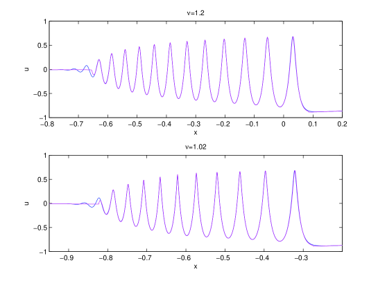
Fig. 9: CH solution (blue) and asymptotic solution (magenta) for the initial datum $u_{0}=-\mbox{sech}^{2}x$ and $\epsilon=10^{-2}$ for $t=1$ and two values of $\nu$

The asymptotic solution is so close to the approached solution that one can only see discrepancies near the boundary of the Whitham zone, where the asymptotic solution is just $C^{0}$. Thus one has to consider the difference between the solutions as shown in Fig. 10. The quality of the numerics allows the study of the scaling behavior at various points in the Whitham zone.

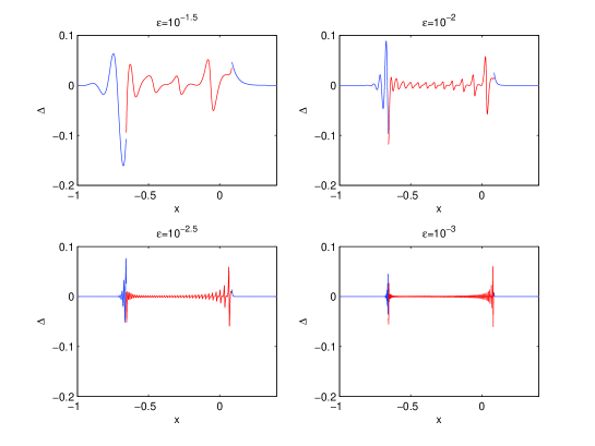
Fig. 10: Difference of the CH solution and the asymptotic solution for the initial datum $u_{0}=-\mbox{sech}^{2}x$ and $\nu=1.2$ for $t=1$ for several values of $\epsilon$. In the Whitham zone (red), the asymptotic solution is given in terms of the one-phase CH solution solution, outside by the solution to the Hopf equation with the same initial datum.

Interior of the Whitham zone:
If we study the $\epsilon$-dependence of the $L_{\infty}$-norm of the difference near the middle of the Whitham zone (we take the maximum of this difference near the geometric midpoint), we find that the norm scales as $\epsilon$. More precisely we find an exponent $a=0.9$ with correlation coefficient $r=0.999$ and standard deviation $\sigma_{a}=0.04$. There is obviously a certain arbitrariness in our definition of this error especially for larger values of $\epsilon$, where there are only few oscillations. In these cases the errors are read off close to the boundaries of the Whitham zone where much smaller exponents for the error are observed (see below). This scaling gives nonetheless strong support for the conjectured form of the phase of the one-phase solution in the Whitham zone, since even a small analytical error in the phase would lead to large errors which would not decrease with $\epsilon$.

Leading edge of the Whitham zone:
Oscillations can always be found outside the Whitham zone, whereas the Hopf solution does not show any oscillations. The biggest difference always occurs at the boundary of the Whitham zone. It scales as $\epsilon^{1/3}$. More precisely we find in the Hopf zone $a=0.33$ with $r=0.99$ and $\sigma_{a}=0.04$. In the interior of the Whitham zone, $a$ has a similar value, but the correlation is worse. If one studies the scaling of the zone, where the difference between Hopf and CH solution near the leading edge has absolute value larger than some treshold (we use $10^{-4}$), we find a decrease compatible with $\epsilon^{2/3}$, more precisely $a=0.81$ with $r=0.99$ and $\sigma_{a}=0.07$.

Trailing edge of the Whitham zone:
The biggest difference is always found at the boundary of the Whitham zone. Its scaling is compatible with $\epsilon^{1/2}$. We find $a=0.51$ with $r=0.9997$ and $\sigma_{a}=0.01$.

6 Numerical study of the multiscales expansion for the CH equation

In this section we study numerically the multiscales solution to CH derived in section 4. It will be shown that the latter provides a better description of the asymptotic behavior near the leading edge of the Whitham zone than the Hopf or the one-phase solution to CH as discussed in section 5. We identify the zone, where the latter gives a better description of CH than the former and study the $\epsilon$-dependence of the errors. For the numerical computation of the Hastings-McLeod solution and a comparison to the KdV case, we refer the reader to [18].

In Fig. 11 we show the CH solution, the asymptotic solution via Whitham and Hopf and the multiscales solution near the leading edge of the Whitham zone. It can be seen that the one-phase solution gives a very good description in the interior of the Whitham zone as discussed in section 5, whereas the multiscales solution gives as expected a better description near the leading edge.

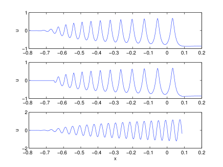
Fig. 11: The figure shows in the upper part the numerical solution to the CH equation for the initial datum $u_{0}=-\mbox{sech}^{2}x$ and $\nu=1.2$, $\epsilon=10^{-2}$ at $t=1$, in the middle the corresponding asymptotic solution in terms of Hopf and one-phase solution, and in the lower part the multiscales solution.

In Fig. 12 the CH and the multiscales solution are shown in one plot for $\epsilon=10^{-2}$. It can be seen that the agreement near the edge of the Whitham zone is so good that one has to study the difference of the solutions. The solution only gives locally an asymptotic description and is quickly out of phase for larger distances from the leading edge.

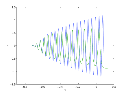
Fig. 12: The numerical solution to the CH equation for the initial datum $u_{0}=-\mbox{sech}^{2}x$ and $\nu=1.2$, $\epsilon=10^{-2}$ at $t=1$ in blue and the corresponding multiscales solution in green.

The difference between CH and multiscales solution is shown for several values of $\epsilon$ in Fig. 13. It can be seen that the maximal error still occurs close to the Whitham edge, but that it decreases much faster with $\epsilon$ than the error given by the Hopf and the Whitham solution. A linear regression analysis for the logarithm of the difference $\Delta$ between CH and multiscales solution near the edge gives a scaling of the form $\Delta\propto\epsilon^{a}$ with $a=0.58$ with standard deviation $\sigma_{a}=0.17$. Since there are much less oscillations in the CH case than in KdV, the found statistics is considerably worse in the former case than in the latter [18], which is reflected by the low correlation coefficient $r=0.93$ and the comparatively large standard deviation. Nonetheless the found scaling is in accordance with the $\epsilon^{2/3}$ scaling expected from the multiscales expansion.

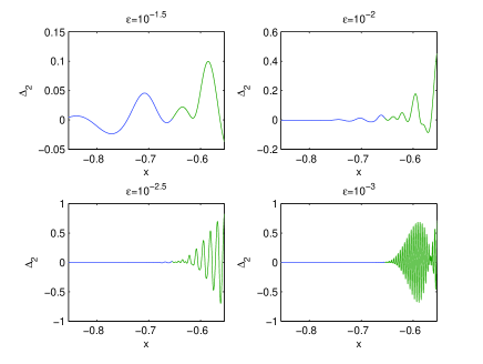
Fig. 13: The difference between the numerical solution to the CH equation for the initial datum $u_{0}=-\mbox{sech}^{2}x$ and $\nu=1.2$ at $t=1$ and the corresponding multiscales solution for 4 values of $\epsilon$. The interior of the Whitham zone is shown in green, the exterior in blue.

As can be already seen from Fig. 11, the multiscales solution gives a better asymptotic description of CH near the leading edge of the Whitham zone than the Hopf and the one–phase solution. This is even more obvious in Fig. 14 where the difference between CH and the asymptotic solutions is shown.

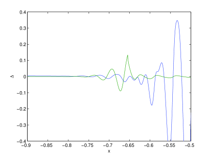
Fig. 14: The difference between the numerical solution to the CH equation for the initial datum $u_{0}=-\mbox{sech}^{2}x$ and $\nu=1.2$, $\epsilon=10^{-2}$ at $t=1$ for $\epsilon=10^{-2}$ and the corresponding multiscales solution in blue, and the difference between CH and Hopf and one-phase solution in green.

This suggests to identify the regions where each of the asymptotic solutions gives a better description of CH than the other. The results of this analysis can be seen in Fig. 15. This matching procedure clearly improves the CH description near the leading edge.

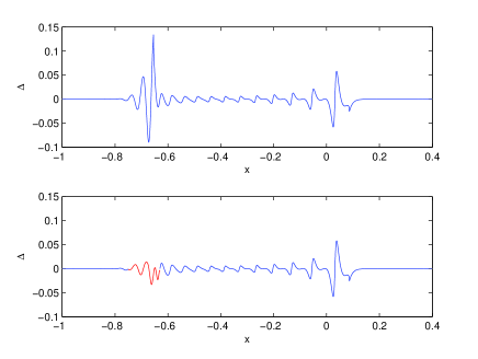
Fig. 15: In the upper part one can see the difference between the numerical solution to the CH equation for the initial datum $u_{0}=-\mbox{sech}^{2}x$ and $\nu=1.2$, $\epsilon=10^{-2}$ at $t=1$ and the corresponding asymptotic solution in terms of Hopf and one-phase solution. The lower figure shows the same difference, which is replaced close to the leading edge of the Whitham zone by the difference between CH solution and multiscales solution (shown in red where the error is smaller than the one shown above).

In Fig. 16 we see the difference between this matched asymptotic solution and the CH solution for two values of $\epsilon$. Visibly the zone, where the solutions are matched, decreases with $\epsilon$.

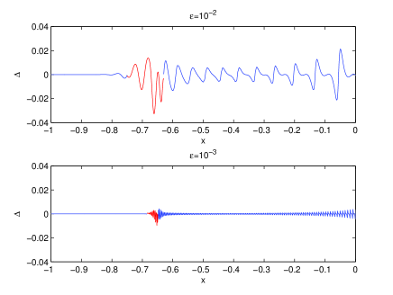
Fig. 16: The difference between the numerical solution to the CH equation for the initial datum $u_{0}=-\mbox{sech}^{2}x$ and $\nu=1.2$ at $t=1$ and the corresponding asymptotic solution in terms of Hopf and one-phase solution in blue and CH and multiscales solution in red, where the latter error is smaller than the former, for two values of $\epsilon$.

There is a certain ambiguity in the precise definition of this matching zone due to the oscillatory character of the solutions. Because of the much lower number of oscillations than in KdV, the statistics is considerably worse in the CH case than in the KdV case. The limits of the matching zone for several values of $\epsilon$ can be seen in Fig. 17. Due to the lower number of oscillations in the Hopf region, the matching zone extends much further into this region than in the Whitham region. The width of this zone scales like $\epsilon^{a}$ with $a=0.51$ and standard deviation $\sigma_{a}=0.06$ and correlation coefficient $r=0.99$.

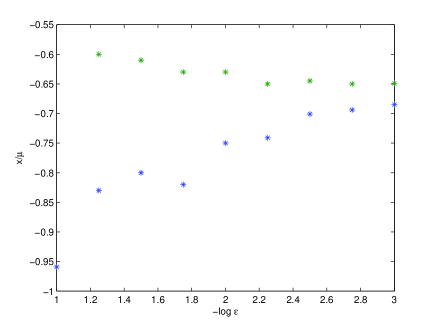
Fig. 17: The edges of the zone where the multiscales solutions provides a better asymptotic description of CH than the Hopf or the one–phase solution for the initial datum $u_{0}=-\mbox{sech}^{2}x$ and $\nu=1.2$ at $t=1$ in dependence of $\epsilon$.

References

- [1] S. Abenda and T. Grava, Modulation of the Camassa–Holm equation and reciprocal transformations, Annales de l’Inst. Fourier - Grenoble, 55(6) (2005), pp. 1803-1834.
- [2] S. Abenda, T. Grava and C. Klein, On Whitham equations for Camassa–Holm, in WASCOM2005, World Scientific Publ. Co (2006), pp. 1–6.
- [3] M. S. Alber and Yu. N. Fedorov, Wave solutions of evolution equations and Hamiltonian flows on nonlinear subvarieties of generalized Jacobians, J. Phys. A 33 (2000), no. 47, pp. 8409–8425.
- [4] V. Busuioc, On second grade fluids with vanishing viscosity., C. R. Acad. Sci. Paris Sr. I Math. 328 (1999), no. 12, pp. 1241–1246.
- [5] R. Camassa R. and D. D. Holm An integrable shallow water equation with peaked solitons Phys. Rev. Lett., 71, (1993), pp. 1661–1664.
- [6] A. Constantin, On the scattering problem for the Camassa-Holm equation., R. Soc. Lond. Proc. Ser. A Math. Phys. Eng. Sci. 457 (2001), pp. 953–970.
- [7] A. Constantin and J. Lenells, On the inverse scattering approach for an integrable shallow water wave equation, Phys. Lett. A 308 (2003), no. 5-6, pp. 432–436.
- [8] S. M. Cox and P. C. Matthews, Exponential time differencing for stiff systems, J. Comput. Phys., 176(2) (2002), pp. 430-455.
- [9] H. H. Dai, Model equations for nonlinear dispersive waves in a compressible Mooney-Rivlin rod. Acta Mech. 127 (1998), no. 1-4, pp. 193–207.
- [10] P. Deift, S. Venakides, and X. Zhou, New result in small dispersion KdV by an extension of the steepest descent method for Riemann-Hilbert problems, IMRN 6, (1997), pp. 285-299.
- [11] B. Dubrovin, On Hamiltonian Perturbations of Hyperbolic Systems of Conservation Laws, II: Universality of Critical Behaviour, Comm. Math. Phys., 267 (2006), pp. 117–139.
- [12] B.A. Dubrovin, Theta-functions and nonlinear equations, Russian Math. Surveys 36 (1981), no. 2(218), pp. 11–80.
- [13] H. R. Dullin, G. A. Gottwald and D. D. Holm, An integrable shallow water equation with linear and nonlinear dispersion, Phys. Rev. Lett. 87 (2001), no. 19, pp. 1661–1664.
- [14] G. Falqui, On a Camassa-Holm type equation with two dependent variables, J. Phys. A 39 (2006), no. 2, pp. 327–342.
- [15] B. Fuchssteiner and A. S. Fokas, Symplectic structures, their Bäcklund transformations and hereditary symmetries, Phys. D 4 (1981/82), no. 1, pp. 47–66.
- [16] T. Grava and C. Klein, Numerical solution of the small dispersion limit of Korteweg de Vries and Whitham equations, Comm. Pure Appl. Math. 60(11) (2007), pp. 1623-1664.
- [17] T. Grava and C. Klein, ‘Numerical study of a multiscale expansion of KdV and Camassa-Holm equation’, in Integrable Systems and Random Matrices, ed. by J. Baik, T. Kriecherbauer, L.-C. Li, K.D.T-R. McLaughlin and C. Tomei, Contemp. Math. Vol. 458,(2008) pp. 81-99 .
- [18] T. Grava and C. Klein, Numerical study of a multiscale expansion of the Korteweg de Vries equation, Proc. Royal. Soc. A 464 (2008), pp. 733-755.
- [19] T. Grava, V. U. Pierce and Fei-Ran Tian, Initial value problem of the Whitham equations for the Camassa-Holm equation, Physica D, 238 1, (2009), pp. 55-66.
- [20] A. G. Gurevich and L. P. Pitaevskii, Non stationary structure of a collisionless shock waves, JEPT Letters 17 (1973), pp. 193-195.
- [21] S. P. Hastings and J. B. McLeod, A boundary value problem associated with the second Painlev transcendent and the Korteweg- de Vries equation, Arch. Rational Mech. Anal. 73 (1980), no. 1, pp. 31–51.
- [22] H. P. McKean, Fredholm determinants and the Camassa-Holm hierarchy. Comm. Pure Appl. Math. 56 (2003), no. 5, pp. 638–680.
- [23] H. P. McKean, Breakdown of the Camassa-Holm equation. Comm. Pure Appl. Math. 57 (2004), no. 4, pp. 416–418.
- [24] C. Klein, Fourth order time-stepping for low dispersion Korteweg-de Vries and nonlinear Schrödinger equation, ETNA 29 (2008), pp. 116-135.
- [25] P. D. Lax and C. D. Levermore, The small dispersion limit of the Korteweg de Vries equation, I,II,III, Comm. Pure Appl. Math. 36 (1983), pp. 253-290, 571-593, 809-830.
- [26] B. Minchev and W. Wright, A review of exponential integrators for first order semi-linear problems, Technical Report 2, The Norwegian University of Science and Technology (2005).
- [27] F. R. Tian, Oscillations of the zero dispersion limit of the Korteweg-de Vries equation, Comm. Pure Appl. Math. 46 (1993), pp. 1093–1129.
- [28] F. R. Tian, The initial value problem for the Whitham averaged system, Comm. Math. Phys. 166 (1994), pp. 79-115.
- [29] L. N. Trefethen, Spectral Methods in MATLAB, SIAM, Philadelphia, 2000.
- [30] S. P. Tsarev, Poisson brackets and one–dimensional Hamiltonian systems of hydrodynamic type. Dokl. Akad. Nauk. SSSR 282 (1985), pp. 534–537.
- [31] S. Venakides, The Korteweg de Vries equations with small dispersion: higher order Lax- Levermore theory, Comm. Pure Appl. Math. 43 (1990), pp. 335–361.
- [32] E. T. Whittaker and G. N. Watson, A course in modern analysis, Cambridge Univ. Press (1952).