Phase transitions in self-dual generalizations of the Baxter-Wu model

Abstract

We study two types of generalized Baxter-Wu models, by means of transfer-matrix and Monte Carlo techniques. The first generalization allows for different couplings in the up- and down triangles, and the second generalization is to a $q$-state spin model with three-spin interactions. Both generalizations lead to self-dual models, so that the probable locations of the phase transitions follow. Our numerical analysis confirms that phase transitions occur at the self-dual points. For both generalizations of the Baxter-Wu model, the phase transitions appear to be discontinuous.

I Introduction

In general, systems in the universality class of the two-dimensional 4-state Potts model display critical singularities that are modified by logarithmic correction factors. A satisfactory explanation of this fact is provided by the renormalization scenario due to Nienhuis et al. NBRS . It explains the logarithmic factors NS as arising from the second temperature field, which is marginally irrelevant. It also shows that the 4-state Potts behavior without logarithmic factors can only occur at special points in the parameter space, where the two leading temperature fields simultaneously vanish. The exactly solved Baxter-Wu model BW precisely fits such a location in parameter space: it belongs to the 4-state Potts class and its leading critical singularities do not have logarithmic factors. Its reduced Hamiltonian reads

$$\beta{\mathcal{H}}=-K^{\rm I}\sum_{\hbox{\raise 0.0pt\hbox{$\bigtriangleup$}}\hbox{\raise 1.50694pt\hbox{$\bigtriangledown$}}}s_{i}s_{j}s_{k}$$ (1)

where $\beta=1/(k_{B}T)$ is the inverse temperature, and the sum is over the up- and down triangles of the triangular lattice, and the site labels $i$, $j$ and $k$ refer to the three spins at the vertices of each triangle. Each spin assumes the Ising values $\pm 1$; this is emphasized by the superscript I of the coupling $K^{\rm I}$. At low temperatures, the model is in one of four long-range ordered phases, where most triangles have an even number of $-$ spins. While the common type of interaction between spins in magnetic materials is of the two-spin type, three-particle interactions such as in the Baxter-Wu model have been used to describe the shape of face-centered cubic crystal surfaces BaN .

This work investigates two different generalizations of the Baxter-Wu model. First we consider the case that the couplings in the up- and down triangles are different (see Fig. 1), i.e.,

$$\beta{\mathcal{H}}=-K^{\rm I}_{1}\sum_{\hbox{\raise 0.0pt\hbox{$\bigtriangleup$}}}s_{i}s_{j}s_{k}-K^{\rm I}_{2}\sum_{\hbox{\raise 1.50694pt\hbox{$\bigtriangledown$}}}s_{i}s_{j}s_{k}$$ (2)

where the sums are over the up- and down triangles of the triangular lattice respectively. The introduction of another temperature-like parameter makes it likely that this model will have a critical line parametrized by the ratio of $K^{\rm I}_{1}$ and $K^{\rm I}_{2}$. The fourfold degeneracy of the ground state persists for $K^{\rm I}_{1}\neq K^{\rm I}_{2}$, so that it may seem plausible that the model still belongs to the 4-state Potts universality class. We shall attempt to provide a more definite judgment by means of a numerical investigation.

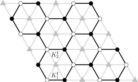
Figure 1: A $6\times 6$ triangular lattice. The lattice is divided into a honeycomb (open and filled circles) and a triangular sublattice (pentagons), which are dual to each other. The honeycomb lattice is bipartite.

For the second generalization it is useful to write Eq. (1) in terms of two-state Potts variables $\sigma_{i}\equiv(s_{i}+3)/2=1$ or 2:

$$\beta{\mathcal{H}}=-K\sum_{\hbox{\raise 0.0pt\hbox{$\bigtriangleup$}}\hbox{\raise 1.50694pt\hbox{$\bigtriangledown$}}}\delta_{2}(\sigma_{i}+\sigma_{j}+\sigma_{k})$$ (3)

where $\delta_{2}(x)=0$ if $x$ is odd and 1 if $x$ is even, and $K=2K^{\rm I}$. The sum is over all up- and down triangles. Eqs. (1) and (3) differ by an additive constant that is irrelevant for the present purposes. It is now straightforward to generalize the model in terms of $q$-state variables with values $\sigma_{i}=1,~{}2,~{}\cdots,~{}q$:

$$\beta{\mathcal{H}}=-K\sum_{\hbox{\raise 0.0pt\hbox{$\bigtriangleup$}}\hbox{\raise 1.50694pt\hbox{$\bigtriangledown$}}}\delta_{q}(\sigma_{i}+\sigma_{j}+\sigma_{k})$$ (4)

where $\delta_{q}(x)=1$ if $(x\mod q)=0$ and $\delta_{q}(x)=0$ otherwise. This model can also be considered as a generalization of the $q$-state Potts model RBP to 3-spin interactions, because the pair couplings of the original Potts model on a bipartite lattice can be written as $-K\delta_{q}(\sigma_{i}+\sigma_{j})$. But the model (4) does not obey the $q$-fold permutation symmetry ${\mathcal{S}}_{q}$ of the Potts model for general $q$. Its symmetry group is ${\mathcal{Z}}_{q}\otimes{\mathcal{Z}}_{q}\otimes{\mathcal{Z}}_{2}\otimes{\mathcal{S}}_{3}$ where the $q$-state clock symmetries ${\mathcal{Z}}_{q}$ are generated by the operation $\sigma_{i}\to\sigma_{i}+1\mod q$, independently for two of the three sublattices, ${\mathcal{Z}}_{2}$ is generated by the operation $\sigma_{i}\to q+1-\sigma_{i}$ on all sites, and ${\mathcal{S}}_{3}$ is the symmetric group of the permutations of the three sublattices. The latter symmetry results from the spatial symmetries of the lattice, namely reflection and translation or rotation, which can permute the three sublattices, while leaving $\beta{\mathcal{H}}$ invariant.

It is obvious that the degeneracy of the ground state increases as $q^{2}$ with the number $q$ of spin states, so that one may expect that the model will display a discontinuous ordering transition for $q>2$. However, the special nature of the critical Baxter-Wu model, i.e. the model of Eq. (4) for $q=2$, namely the vanishing of the marginal temperature field, opens the possibility of another scenario. After a mapping on the Coulomb gas BN , the marginal temperature field translates into the fugacity of the $e=4$ electric charges. Thus the $q=2$ transition maps precisely on the point of the Gaussian fixed line where the electric charges are absent, and there seems to be a real possibility that this is also the case for other values of $q$. Since one expects that the Coulomb gas coupling increases with $q$, the electric charges, which are marginal at $q=2$, must be relevant for $q>2$, and would drive the ordering transition first order. But, if these charges remain absent, the transition still takes place on the Gaussian line, and must be critical.

For this reason it is interesting to investigate the character of the ordering transition for $q>2$. There are existing results due to Alcaraz et al. AJ ; ACO who investigated a different generalization of the Baxter-Wu model, namely, to a $p$-state clock model. For the case $p=3$, their model is equivalent with our $q=3$ model. They concluded that the transition is first-order for $p=3$, on the basis of approximate renormalization calculations, and Monte Carlo calculations starting in the ordered and the disordered states, displaying changes of phase.

The property of self-duality plays an important role in the present work, because knowledge of the critical point greatly facilitates the numerical analyses. Its derivation is the subject of Sec. II where we formulate a relatively simple proof of self-duality for a class of models that includes both generalizations of the Baxter-Wu model mentioned above. In Sec. IV we present our numerical analysis of the $q=2$ model with two different couplings, and in Sec. V we report our findings for the $q=3$ and 4 models with uniform couplings. The conclusions of our analyses are listed in Section VI.

II Duality of $q$-state models with multispin interactions

Self-duality is a useful tool to locate phase transitions. If a single phase transition occurs as a function of temperature, then the transition must occur at the point where the temperature variable $K$ and the dual temperature variable $\tilde{K}$ coincide. In the case of self-dual models with two variables $K_{1}$ and $K_{2}$, the transitions tend to occur on the self-dual line in the $K_{1},K_{2}$ plane, i.e., in a point that maps onto itself under duality.

Duality was first found for the square-lattice Ising model by Kramers and Wannier KraWa , who correctly predicted the critical point at

$$K^{\rm I}_{\rm c}=\frac{1}{2}\ln(1+\sqrt{2})$$ (5)

and since then many more derivations have been reported. Gruber et al. GHM have formulated a very general proof that includes all systems studied in the present work. For the convenience of the reader we shall provide a simple proof that is less general than that of Gruber et al. GHM , but still more general than actually required for the models under the present investigation.

Simpler, and less general versions of the proof given by Gruber et al. appear elsewhere in the literature. Examples are the two-dimensional Ising model with pair interactions in one direction and multispin interactions in the perpendicular direction (see Refs. Turban , and ZY for a generalization to $q>2$ Potts models with similar interactions).

The present derivation of self-duality applies to a system of $q$-state variables located on a simple hypercubic lattice. The variables are denoted $\sigma_{{\mathbf{r}}}$ and take the values $1,\cdots,q$. Their interactions are described by a Hamiltonian of the general form

$$-\beta{\mathcal{H}}=K_{1}\sum_{{\mathbf{r}}}\delta_{q}\left(\sum_{i=1}^{n}\sigma_{{\mathbf{r}}+{\mathbf{a}}_{i}}\right)+K_{2}\sum_{{\mathbf{r}}}\delta_{q}\left(\sum_{j=1}^{m}\sigma_{{\mathbf{r}}+{\mathbf{b}}_{j}}\right)$$ (6)

where ${\mathbf{r}}$ is a lattice vector and ${\mathbf{a}}_{i}$ and ${\mathbf{b}}_{j}$ are vectors pointing from position ${\mathbf{r}}$ to the sites of the variables participating in the interaction assigned to site ${\mathbf{r}}$. There are two multiparticle interactions per site, one with $n$ participating sites and another with $m$ sites. The class includes the square-lattice Potts model with nearest-neighbor interactions, after a suitable renaming $\sigma\to q-\sigma$ of the $q$ states on one of the two sublattices. It also includes the Baxter-Wu model for $n=m=3$, $a_{1}=-b_{1}=(0,0)$, $a_{2}=-b_{2}=(1,0)$, $a_{3}=b_{3}=(0,1)$, $q=2$, and $K_{1}=K_{2}$. The partition function for our class of models takes the form:

$$Z(v_{1},v_{2})=\sum_{\{\sigma_{{\mathbf{r}}}\}}\prod_{{\mathbf{r}}}\left[1+v_{1}\delta_{q}\left(\sum_{i=1}^{n}\sigma_{{\mathbf{r}}+{\mathbf{a}}_{i}}\right)\right]\left[1+v_{2}\delta_{q}\left(\sum_{j=1}^{m}\sigma_{{\mathbf{r}}+{\mathbf{b}}_{j}}\right)\right],$$ (7)

where $v_{1}=\exp(K_{1})-1$ and $v_{2}=\exp(K_{2})-1$. Each $\delta_{q}$-function in Eq. (7) can be substituted by its Fourier representation

$$\delta_{q}(z)=\frac{1}{q}\sum_{t=1}^{q}e^{\pm 2\pi izt/q}\,,$$ (8)

and each “1” in Eq. (7) can be replaced using the identity

$$1=\sum_{t=1}^{q}\delta_{q}(t)e^{\pm 2\pi izt/q}\;.$$ (9)

The effect of these substitutions is that two new variables $t_{{\mathbf{r}}}$ and $t^{\prime}_{{\mathbf{r}}}$ are introduced on each site ${\mathbf{r}}$, for the $n$- and $m$-particle interactions, respectively. This leads to

$$Z(v_{1},v_{2}) = \sum_{\{\sigma\}}\prod_{{\mathbf{r}}}\sum_{\{t_{{\mathbf{r}}},t^{\prime}_{{\mathbf{r}}}\}}[\delta_{q}(t_{{\mathbf{r}}})+\frac{v_{1}}{q}\,][\delta_{q}(t^{\prime}_{{\mathbf{r}}})+\frac{v_{2}}{q}\,]$$ (10)

$$\exp\left[\frac{2\pi i}{q}\left(t_{{\mathbf{r}}}\sum_{i=1}^{n}\sigma_{{\mathbf{r}}+{\mathbf{a}}_{i}}-t^{\prime}_{{\mathbf{r}}}\sum_{j=1}^{m}\sigma_{{\mathbf{r}}+{\mathbf{b}}_{j}}\right)\right]\;.$$

After reordering the summations and the products and collecting terms with the same $\sigma$, we obtain

$$Z(v_{1},v_{2}) = (v_{1}v_{2}/q)^{N}\sum_{\{t,t^{\prime}\}}\prod_{{\mathbf{r}}}[1+(q/v_{1})\delta_{q}(t_{{\mathbf{r}}})][1+(q/v_{2})\delta_{q}(t^{\prime}_{{\mathbf{r}}})]$$ (11)

$$\sum_{\{\sigma\}}(1/q)\exp\left[(2\pi i\sigma_{{\mathbf{r}}}/q)\left(\sum_{i=1}^{n}t_{{\mathbf{r}}-{\mathbf{a}}_{i}}-\sum_{j=1}^{m}t^{\prime}_{{\mathbf{r}}-{\mathbf{b}}_{j}}\right)\right]\;,$$

where $N$ is the total number of sites in the lattice. A nice property of Eq. (11) is that the degrees freedom $\sigma_{{\mathbf{r}}}$ on different sites ${\mathbf{r}}$ are completely independent, and thus the summation over the $\sigma_{{\mathbf{r}}}$ becomes very easy. Using again Fourier-transformation (8), one has

$$Z(v_{1},v_{2}) = (v_{1}v_{2}/q)^{N}\sum_{\{t_{{\mathbf{r}}},t^{\prime}_{{\mathbf{r}}}\}}\prod_{{\mathbf{r}}}[1+(q/v_{1})\delta_{q}(t_{{\mathbf{r}}})][1+(q/v_{2})\delta_{q}(t^{\prime}_{{\mathbf{r}}})]$$ (12)

$$\delta_{q}\left(\sum_{i=1}^{n}t_{{\mathbf{r}}-{\mathbf{a}}_{i}}-\sum_{j=1}^{m}t^{\prime}_{{\mathbf{r}}-{\mathbf{b}}_{j}}\right)\;.$$

In short, the original $q$-valued variable $\sigma_{{\mathbf{r}}}$ has been integrated out. The price paid is the introduction on each site of two new $q$-valued variables $t_{{\mathbf{r}}},t^{\prime}_{{\mathbf{r}}}$ with an additional $\delta$-function constraint.

Next, one introduces a new $q$-state variable $\tilde{\sigma}_{{\mathbf{r}}}$ on each site, and let $t$:

$$t_{{\mathbf{r}}}=\sum_{j=1}^{m}\tilde{\sigma}_{{\mathbf{r}}-{\mathbf{b}}_{j}}\bmod q,$$ (13)

which will be feasible for appropriate boundary conditions. The $\delta$ function connecting $t_{{\mathbf{r}}}$ and $t^{\prime}_{{\mathbf{r}}}$ in Eq. (12) is satisfied if

$$t^{\prime}_{{\mathbf{r}}}=\sum_{i=1}^{n}\tilde{\sigma}_{{\mathbf{r}}-{\mathbf{a}}_{i}}\bmod q\;.$$ (14)

As the number of new variables $\tilde{\sigma}_{{\mathbf{r}}}$ is equal to the number of old variables $t$ and $t^{\prime}$ reduced by the number of constraints on $t$ and $t^{\prime}$ imposed by the rightmost $\delta$ function in Eq. (12), we expect that the $\tilde{\sigma}_{{\mathbf{r}}}$ are determined up to a trivial shift. After an inversion of the lattice, Eq. (12) takes the form

$$Z(v_{1},v_{2})=\left(\frac{v_{1}v_{2}}{q}\right)^{N}\sum_{\{\tilde{\sigma}_{{\mathbf{r}}}\}}\prod_{{\mathbf{r}}}\left[1+\frac{q}{v_{2}}\,\delta_{q}\left(\sum_{i=1}^{n}\tilde{\sigma}_{{\mathbf{r}}+{\mathbf{a}}_{i}}\right)\right]\left[1+\frac{q}{v_{1}}\,\delta_{q}\left(\sum_{j=1}^{m}\tilde{\sigma}_{{\mathbf{r}}+{\mathbf{b}}_{j}}\right)\right],$$ (15)

Comparison with Eq. (7) shows that $Z(v_{1},v_{2})$ satisfies the self-duality relation

$$Z(v_{1},v_{2})=\left(\frac{v_{1}v_{2}}{q}\right)^{N}Z(\tilde{v}_{1},\tilde{v}_{2})\hskip 56.9055pt\mbox{with}\hskip 14.22636ptv_{1}\tilde{v}_{2}=q\,,~{}~{}v_{2}\tilde{v}_{1}=q\;.$$ (16)

The dual set of coupling constants $(\tilde{K}_{1},\tilde{K}_{2})$ obey

$$\tilde{v}_{1}=e^{\tilde{K}_{1}}-1\hskip 28.45274pt\mbox{and}\hskip 28.45274pt\tilde{v}_{2}=e^{\tilde{K}_{2}}-1\;.$$ (17)

Each point on the line

$$v_{1}v_{2}=q$$ (18)

is mapped onto itself, and we find, for the case $v_{1}=v_{2}$ the symmetric self-dual point as $v=\sqrt{q}$ or

$$K=\ln(1+\sqrt{q})\,.$$ (19)

In this self-dual point the average number of satisfied multiparticle interactions (“satisfied” means that the sum modulo $q$ of the spins coupled by the interaction vanishes) per site, if unique, is found from the derivative of $\ln Z$ with respect to the coupling constants at the self-dual point. In the case of a first-order transition on the self-dual line, this yields the mean of the values in the disordered phase and in the ordered phase.

For $q=2$ models defined in terms of Ising spins $s_{i}=\pm 1$, one has to take into account the factor 2 between the “Potts” and “Ising” couplings, as appearing under Eq. (3)–i.e., $v=\exp(2K^{\rm I})-1$. In the Ising case, the equation for the self-dual line Eq. (18) may be written as

$$\sinh(2K^{\rm I}_{1})\sinh(2K^{\rm I}_{2})=1$$ (20)

In many cases, the self-dual line, or a part of it, is the locus of a phase transition. The existence, uniqueness, and character of a phase transition, however, are not determined by self-duality. For that purpose, additional calculations are required. For several Ising models with multispin interactions and a field ($m=1$), including three-dimensional models, Blöte et al. sedua found discontinuous transitions on a part of the self-dual line, with a gas-liquid like critical point at the end of the first-order range. For a two-dimensional system with pair interactions in one direction and multiparticle interactions between $p$ particles in the perpendicular direction, Zhang and Yang ZY concluded, from Monte Carlo calculations, that a phase transition occurs at the self-dual point, and that it is first-order for all $q>2$ if $p>2$. Also in the case of the $n$-state clock model with three-particle interactions on the triangular lattice, Alcaraz et al. found from Monte Carlo calculations AJ that phase transitions occur at the self-dual points for $n=2$ and $n=3$.

III Numerical Methods

We investigate the generalized Baxter-Wu model (6) on the triangular lattice, both by transfer-matrix method and by Monte Carlo simulations.

III.1 Transfer-matrix

The transfer-matrix techniques used in this work are adequately described in the literature, although the information is divided over different papers. The essential parts are explained in Refs. MPN , BN1982 and QWB . Here we only add a few general and specific remarks for the convenience of the reader. From a few of the leading eigenvalues of the transfer matrix, one can calculate the free energies, the magnetic and energy-like correlation lengths of $L\times\infty$ systems. For the case $q=2$ we could perform such calculations up to finite sizes $L=27$. The geometry is that of the triangular lattice wrapped on a cylinder, with one set of edges perpendicular to the axis of the cylinder. The finite size $L$ is specified such that the circumference of the cylinder is spanned by $L$ lattice edges.

Here we use the true triangular lattice, instead of the representation as a square lattice with one set of diagonal bonds, as used in Sec. II. Since, after adding one layer of spins, the lattice is shifted by a half lattice unit along the finite direction, we chose a transfer matrix that adds two layers of spins and applies an additional reverse shift operation, in order to ensure that the transfer matrix commutes with the lattice reflection as specified below. Such commutation relations allow one to find a common set of eigenstates of the transfer matrix and a symmetry operator.

The transfer matrix acts on a vector space with vector indices representing the state of a row of $L$ Ising spin variables. For $q=2$, the vector indices can thus be written as binary numbers $b_{L}b_{L-1}\cdots b_{2}b_{1}$ with $b_{k}\equiv(s_{k}+1)/2$. For $q=3$ one uses ternary numbers, etc., but here we shall use the language for binary numbers. The transfer matrix calculations focus on three eigenvalues, namely the largest one $\lambda_{0}$, the ”magnetic” one $\lambda_{m}$, and the ”thermal” eigenvalue $\lambda_{t}$. These eigenvalues are defined in the usual way, by means of the group of symmetry operations that leave the Hamiltonian invariant, but permute the ordered phases. The thermal eigenvalue, like the largest eigenvalue corresponds to an eigenvector fully invariant under these symmetry operations. The magnetic eigenvalue is the largest one with an eigenvector that changes under these symmetry operations. In this model the relevant symmetry group is generated by the allowed permutations of the $q$ states, and by lattice symmetries that permute the three sublattices. As the transfer matrix breaks some of the latter symmetries, we replace the full symmetry group by the subgroup that is not violated by the transfer matrix.

The analyses based on $\lambda_{t}$ and $\lambda_{m}$ are similar. We proceed as follows for the case of $\lambda_{m}$. The magnetic correlation function $g_{m}(r)$ as a function of the distance $r$ in the length direction of the cylinder is defined as $g_{m}(r)=\langle s_{0}s_{r}\rangle$. For sufficiently large $r$, $g_{m}(r)$ decays exponentially on a length scale $\xi_{m}$ that depends on $L$ and the couplings, i.e.,

$$g_{m}(r)\propto{\rm e}^{-r/\xi_{m}(K_{1},K_{2},L)}$$ (21)

and is determined by the eigenvalues $\lambda_{0}$ and $\lambda_{m}$ of the transfer matrix:

$$\xi_{m}^{-1}(K_{1},K_{2},L)=\frac{1}{\sqrt{3}}\ln(\lambda_{0}/\lambda_{m})\,.$$ (22)

The geometric factor $\sqrt{3}$ allows for the thickness of two layers added by the transfer matrix, expressed in the same unit as the finite size $L$. With the help of Cardy’s conformal mapping Cardy-xi of the infinite plane on a cylinder with a circumference $L$, one can now, for a system at criticality, relate the magnetic scaling dimension $X_{h}$, which describes the algebraic decay of the correlation function in the infinite system, to $\xi_{m}$. Defining the scaled gap $X_{h}(K_{1},K_{2},L)$ by

$$X_{h}(K_{1},K_{2},L)\equiv\frac{L}{2\pi\xi_{m}(K_{1},K_{2},L)}\,,$$ (23)

and using finite-size scaling FSS , one finds that, at criticality,

$$X_{h}(K_{1},K_{2},L)=X_{h}+b_{1}L^{y_{1}}+b_{2}L^{y_{2}}+\cdots$$ (24)

where the correction terms $b_{i}L^{y_{i}}$ arise from irrelevant fields, whose presence means that conformal invariance applies only in the limit of large length scales. Since the irrelevant exponents satisfy $y_{i}<0$, $X_{h}(K_{1},K_{2},L)$ converges to $X_{h}$ with increasing $L$, and numerical estimates of $X_{h}$ can be obtained from the finite-size data that can be calculated for a range of system sizes.

For a system that is not critical due to the presence of some relevant scaling field, a term with a positive power of $L$ appears in Eq. (24), which will lead to crossover to different behavior, for instance described by a zero-temperature or an infinite-temperature fixed point. A finite-size analysis of the quantity $X_{h}(K_{1},K_{2},L)$ may thus show whether or not the system is critical, and if so, provide information on the universality class of the model.

The analysis of the temperature dimension $X_{t}$ from the energy-like correlation length $\xi_{t}$ similarly uses the eigenvalue $\lambda_{t}$. The calculation of this eigenvalue, with the same symmetry as $\lambda_{0}$, is described in Ref. BN1982 .

III.2 Monte Carlo algorithm

Simulation of the generalized Baxter-Wu model on the triangular lattice can simply employ the standard Metropolis method which involves single-spin updates only. However, a more efficient algorithm–a Swendsen-Wang-type cluster Monte Carlo method–can be formulated, which was already described for the Baxter-Wu model in Ref. NE .

To construct such a cluster method, one first divides the triangular lattice $\mathcal{T}$ into three sublattices ${\mathcal{L}}_{T_{1}}$, ${\mathcal{L}}_{T_{2}}$, and ${\mathcal{L}}_{T_{3}}$ which are triangular. The union of any two sublattices form a honeycomb lattice ${\mathcal{L}}_{H}$ which is dual to the remaining triangular lattice (see Fig. 1). The partition sum of a generalized Baxter-Wu model can then be written

$$Z(v_{1},v_{2})=\sum_{\{\sigma_{k}\}}\sum_{\{\sigma_{i},\sigma_{j}\}}\prod_{\langle ij\rangle}e^{K_{1}\delta_{q}(\sigma_{i}+\sigma_{j}+\sigma_{k})}e^{K_{2}\delta_{q}(\sigma_{i}+\sigma_{j}+\sigma_{k^{\prime}})}$$ (25)

where the product is over every edge of the honeycomb sublattice ${\mathcal{L}}_{H}$, and $k$ and $k^{\prime}$ are the two neighboring sites on the remaining triangular sublattice, on either side of edge $\langle ij\rangle$. The statistical weight associated with each edge $\langle ij\rangle$ is then

$$e^{K_{1}\delta_{q}(\sigma_{i}+\sigma_{j}+\sigma_{k})}e^{K_{2}\delta_{q}(\sigma_{i}+\sigma_{j}+\sigma_{k^{\prime}})}=$$

$$[1+v_{1}\delta_{q}(\sigma_{i}+\sigma_{j}+\sigma_{k})][1+v_{2}\delta_{q}(\sigma_{i}+\sigma_{j}+\sigma_{k^{\prime}})]=$$

$$\sum_{b_{ij}^{(1)}=0,1}[v_{1}\delta_{q}(\sigma_{i}+\sigma_{j}+\sigma_{k})]^{b_{ij}^{(1)}}\sum_{b_{ij}^{(2)}=0,1}[v_{2}\delta_{q}(\sigma_{i}+\sigma_{j}+\sigma_{k^{\prime}})]^{b_{ij}^{(2)}}$$ (26)

where $v_{1}=\exp(K_{1})-1$ and $v_{2}=\exp(K_{2})-1$, and the convention $0^{0}=1$ has been used. Thus, by introducing two bond variables $b_{ij}^{(1)},b_{ij}^{(2)}$ for every edge of ${\mathcal{L}}_{H}$, and replacing the corresponding edge weights in Eq. (25) according to Eq. (26), one obtains a joint spin-bond model.

The Swendsen-Wang-type cluster method can be adapted to simulate the joint spin-bond model. Two basic steps are involved: the bond- and the spin updates. Given a spin configuration, Eq. (26) tells that the bond updates can be performed as in a uncorrelated bond percolation: the bond-occupation probability is $p=v_{1}/(1+v_{1})$ for $b_{ij}^{(1)}$ on each edge with a satisfied up triangle, and $p=v_{2}/(1+v_{2})$ for $b_{ij}^{(2)}$ on each edge with a satisfied down triangle, and $p=0$ otherwise. Given a bond configuration, Eq. (26) tells that spin configurations satisfying the $\delta$ functions have equal probability. Making use of the fact that the honeycomb lattice is bipartite, one can formulate the following algorithm.
Cluster algorithm, version 1:

1. Sublattice division. Randomly with equal probability label the three sublattices as 1, 2 and 3. Then merge two sublattices into a honeycomb lattice ${\mathcal{L}}_{H}\equiv{\mathcal{L}}_{T_{2}}\cup{\mathcal{L}}_{T_{3}}$.

2. Bond update. On each edge $\langle ij\rangle$ of the honeycomb sublattice ${\mathcal{L}}_{H}$, place an occupied bond with probability $p=1-e^{-K_{1}-K_{2}}$ if both the up- and the down-triangles are satisfied, $p=1-e^{-K_{1}}$ if only the up triangle is satisfied, $p=1-e^{-K_{2}}$ if only the down triangle is satisfied, and $p=0$ otherwise.

3. Cluster construction. A cluster is defined as a group of sites connected through occupied bonds, irrespective of colors. Decompose the lattice ${\mathcal{L}}_{H}$ into clusters (including single-site clusters).

4. Spin update. All the spins on the triangular sublattice ${\mathcal{L}}_{T_{1}}$ are left unchanged. Randomly with uniform probability choose a value $\tau=0,1,2,\cdots,q-1$. Independently for each cluster, update the spins on sublattice ${\mathcal{L}}_{T_{2}}$ according to $\sigma\rightarrow(\sigma+\tau)\mbox{ mod }q$, and the spins on ${\mathcal{L}}_{T_{3}}$ according to $\sigma\rightarrow(\sigma+q-\tau)\mbox{ mod }q$.

This completes one Swendsen-Wang-type cluster step, and a new spin configuration is obtained. Other choices are possible to choose $\tau$ in step 4, for instance $\tau=0$ with probability 1/2 and the other values of $\tau$ with probability $1/(2q-2)$. The choice $\tau=0$ with probability 0 and the other values with probability $1/q$ is only applicable for $q>2$.

For the special case $q=2$ the cluster algorithm can be made more efficient. Conditional on the frozen spin configuration on sublattice ${\mathcal{L}}_{T_{1}}$, the honeycomb sublattice of the $q=2$ generalized Baxter-Wu model reduces to an Ising model with position-dependent couplings on the honeycomb lattice ${\mathcal{L}}_{H}$:

$$\beta{\mathcal{H}}|_{\{\sigma_{k}\},k\in{\mathcal{L}}_{T_{1}}}=-\sum_{\langle ij\rangle}s_{i}s_{j}(K_{1}^{\rm I}s_{k}+K_{2}^{\rm I}s_{k^{\prime}})\equiv-\sum_{\langle ij\rangle}K_{ij}s_{i}s_{j}\hskip 28.45274pt(s=\pm 1)$$ (27)

where the meaning of $k$ and $k^{\prime}$ is the same as in Eq. (25). The effective coupling $K_{ij}$ is defined by the right-hand side of this equation, and can be ferromagnetic or antiferromagnetic, depending on the spin variables $s_{k}$ and $s_{k^{\prime}}$. On the basis of Eq. (27), the “bond-update” step can be reformulated as follows.
Cluster algorithm, version 2:

1. Bond-update. On each edge $\langle ij\rangle$ of ${\mathcal{L}}_{H}$, place an occupied bond with probability $p=\max[0,1-\exp(-2s_{i}s_{j}K_{ij})]$.

The other steps are equal to those of version 1. An occupied bond can be either “ferromagnetic” or “antiferromagnetic” (between spins of opposite signs). A cluster in version 1 may be further decomposed into several clusters in version 2.

We found that version 2 performs much better than the Metropolis algorithm, in the sense that a simulation using the cluster method yields statistically more accurate results in a given time. For the $q=2$ case with $K_{1}=K_{2}$, we found the dynamic exponent $z$ as about $1.1$, which is close to the Li-Sokal bound Li_89 $z\geq 2y_{t}-1=1$. For the self-dual points with $K_{1}\neq K_{2}$, as well as those with $q>2$, a further increase of the slowing down was observed.

We mention that a single-cluster version of the algorithm can also be formulated. However, we found that it does not further improve the efficiency. In fact, for the $q=2$ case with $K_{1}=K_{2}$, the dynamic exponent appears to exceed that of the full cluster-decomposition method.

IV Results for $q=2$ and $K_{1}\neq K_{2}$

For the present case $q=2$ we use the Ising notation for the condition of self-duality as expressed by Eq. (20). Our numerical analysis divides into two parts. The transfer-matrix results are described in subsection IV.1. The Monte Carlo investigation is reported in subsection IV.2.

IV.1 Transfer-matrix results

We calculated the scaled gaps at the self-dual points with $K^{\rm I}_{1}=K^{\rm I}_{2}$, and $K^{\rm I}_{1}=0.5$, 0.6, $\cdots$, 1.2, for system sizes up to $L=27$. The system sizes were restricted to multiples of 3, because otherwise three of the four ground states do not fit in a lattice with period $L$. For the pure Baxter-Wu model at criticality, with $K^{\rm I}_{1}=K^{\rm I}_{2}=[\ln(1+\sqrt{2})]/2$, we find that the finite-size data for the scaled gaps rapidly approach the exact values $X_{h}=1/8$ and $X_{t}=1/2$. Three-point fits according to

$$X_{h}(L)\simeq X_{h}+aL^{p}$$ (28)

followed by iterated fits as described in Ref. BN1982 reproduce the exact values up to about $10^{-7}$. For $K^{\rm I}_{1}\neq K^{\rm I}_{2}$, the finite-size dependence of the scaled gaps becomes stronger while the signs of convergence disappear, at least for a certain range of $K^{\rm I}_{1}/K^{\rm I}_{2}$. This is illustrated by the finite-size data in Table 1.

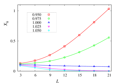
Figure 2: (Color online) Scaled gaps $X_{h}$ a function of system size $L$, for various pairs of couplings ($K^{\rm I}_{1},K^{\rm I}_{2}$) proportional to the self-dual pair with $K^{\rm I}_{1}=1$ (and $K^{\rm I}_{1}=0.13617\cdots$). From top to bottom, the data apply to 0.95, 0.975, 1, 1.025, and 1.05 times the self-dual couplings. These data suggest the presence of a phase transition at or near the self-dual point.

Table 1: Results of transfer-matrix calculations of the scaled magnetic (left hand side) and energy-like (right hand side) gaps at the self-dual points of the generalized Baxter-Wu model for several values of $K^{\rm I}_{1}$. The second column indicates the type $s$ of the scaled gap, $h$ for $X_{h}$ and $t$ for $X_{t}$. The third column shows the scaled gap for the largest available system size $L=27$. Its finite-size dependence is indicated in the fourth column as the difference between the scaled gaps for the two largest finite sizes. The effective exponent $p$ describing the finite-size dependence of the scaled gap is listed in the rightmost column, based on the scaled gaps for $L=21$, 24, and 27. Positive values of $p$ mean that the system is renormalizing away from a fixed point. The values of $X_{h}$ and $X_{t}$ in the first line in this table are close to the exact values of the scaling dimensions; the other entries for $X_{h}$ and $X_{t}$ have no physical meaning except describing the crossover to another fixed point, possibly with $X_{h}=X_{t}=0$.

$K^{\rm I}_{1}$	$X_{h}(27)$	$X_{h}(27)-X_{h}(24)$	$p$	$X_{t}(27)$	$X_{t}(27)-X_{t}(24)$	$p$
0.4407	0.124980	$~{}0.0000058$	$-2.2$	0.500626	$-0.00017$	$-2.0$
0.5	0.124412	$~{}0.0000051$	$-2.3$	0.493960	$-0.00019$	$-2.0$
0.6	0.121082	$-0.000022$	0.47	0.457856	$-0.00047$	$-1.0$
0.7	0.114513	$-0.00018$	0.26	0.398625	$-0.0018$	$-0.23$
0.8	0.103767	$-0.0013$	0.45	0.324382	$-0.0044$	$0.10$
0.9	0.088070	$-0.0017$	0.62	0.244713	$-0.0080$	$0.24$
1.0	0.068388	$-0.0033$	0.83	0.170464	$-0.011$	$0.21$
1.1	0.048182	$-0.0046$	0.42	0.110422	$-0.013$	$0.00$
1.2	0.031335	$-0.0051$	0.00	0.067915	$-0.012$	$-0.37$

These data show that the scaled gaps for the larger system sizes tend to move away from the exact values for the Baxter-Wu model when $K^{\rm I}_{1}$ increases. Moreover, the finite-size dependence, as indicated by the difference of the scaled gaps for the two largest system sizes, increases with $K^{\rm I}_{1}$, except for the entry for $X_{t}$ at largest value $K^{\rm I}_{1}=1.2$. Another significant phenomenon is that the exponent $p$ obtained by the three-point fit for the largest available system is positive for a range of $K^{\rm I}_{1}$, i.e., there are no longer signs of convergence with $L$. Only in the case of $K^{\rm I}_{1}=1.2$ the exponent becomes negative at the largest available system size, which is a sign that the renormalized system is approaching an attractive fixed point.

The presence of a phase transition can be deduced from the scaling behavior of the scaled gaps as a function of temperature. The scaled magnetic gaps were calculated at couplings equal to 0.95, 0.975, 1, 1.025, and 1.05 times the self-dual pair ($K^{\rm I}_{1},K^{\rm I}_{2}$) with $K^{\rm I}_{1}=1.0$. These data are shown in Fig. 2. For the smallest coupling and largest values of $L$ the behavior tends to become linear as a function of $L$, which corresponds with a correlation length $\xi_{m}$ that becomes constant, as expected in a disordered phase. For the largest couplings, the scaled gap tends rapidly to zero, which corresponds with a long-range ordered phase. This crossover with increasing $L$, which is to the high temperature phase or to the ordered phase for ($K^{\rm I}_{1},K^{\rm I}_{2}$) smaller or larger than the self-dual pair respectively, confirms the presence of a phase transition at the self-dual coupling.

IV.2 Monte Carlo results

The evidence that the symmetric Baxter-Wu model ($K_{1}=K_{2}$, $q=2$) undergoes a second-order phase transition is very solid from the exact solution, an exact mapping to the O(2) loop model on the honeycomb lattice DSS , and the existing numerical data.

Using the aforementioned Swendsen-Wang-type cluster algorithm (version 2), we simulated the $q=2$ generalized Baxter-Wu model at the self-dual line with $K_{1}^{\rm I}=0.6$ and $0.8$. The linear system size $L$ was taken as multiples of $6$ in the range $6\leq L\leq 192$; periodic boundary conditions were imposed. Several quantities were sampled, including the number of satisfied up (down) triangles per site $-E_{\rm u}~{}(-E_{\rm d})$, the energy density $E$, the specific heat $C=L^{2}(\langle E^{2}\rangle-\langle E\rangle^{2})$, and the squared magnetization, defined in analogy with the $n_{\rm P}$-state Potts model as

$$m_{\rm P}^{2}=\frac{1}{n_{\rm P}-1}\sum_{i=1}^{n_{\rm P}-1}\sum_{j=i+1}^{n_{\rm P}}(\rho_{i}-\rho_{j})^{2}\;,$$ (29)

where we have divided the satisfied triangles into $n_{\rm P}=q^{2}$ groups according to the associated ground states, and $\rho_{i}$, with $i=1,n_{\rm P}$, is the density of triangles in the $i$th ground state.

We fitted the $C$ data by

$$C(L)=a+bL^{2-2X_{t}}$$ (30)

and the $m_{\rm P}^{2}$ data by

$$m_{\rm P}^{2}(L)=L^{-2X_{h}}(a+bL^{-1})\;,$$ (31)

where $a$ and $b$ are unknown constants. The fits yield $X_{t}=0.43~{}(2)$ and $X_{h}=0.1208~{}(6)$ for $K_{1}^{\rm I}=0.6$, and $X_{t}=0.30~{}(3)$ and $X_{h}=0.110~{}(2)$ for $K_{1}^{\rm I}=0.8$. The results are compatible with those in Table 1.

The probability distributions $P$ for the sampled quantities are also analyzed. The distribution $P(E_{\rm u})$ of the density $-E_{\rm u}$ of the satisfied up-triangles appears to be clearly bimodal, but the two peaks have unequal heights. The reweighted distributions $P_{\rm r}$ were obtained by multiplication of $P(E_{\rm u})$ with a factor $e^{a+bE_{\rm u}}$, with $a$ and $b$ chosen such that $P_{\rm r}(E_{\rm u})$ is normalized to 1 and that its two peaks have equal heights. This transformation takes away an overall gradient in the energy distribution so that the signature of a first order transition is clearly visible. Figure 3 shows $P_{\rm r}$ as a function of $E_{\rm u}$, and the distance $\Delta E_{\rm u}$ between its two maxima.

For first-order transitions, we expect the following behavior of the reweighted energy distribution:

1. The difference between the maximum probability density $\max[P(E_{\rm u})]$ and the local minimum $\min[P(E_{\rm u})]$ between both maxima increases as $L$ increases LK ;

2. The distance $\Delta E_{\rm u}$ approaches to a nonzero value when $L\rightarrow\infty$.

The data shown in Fig. 3 are in agreement with these conditions. The horizontal scale is chosen as $L^{-1/2}$ because $\Delta E_{\rm u}$ then behaves approximately linearly in the pertinent range $24\leq L\leq 384$. For larger $L$ we expect a faster type of convergence, which means that the extrapolation in Fig. 3 may slightly underestimate the energy discontinuity for $L\to\infty$. We also sampled the probability distribution of the magnetization-like quantity $m_{\rm P}^{2}$, and found the same type of behavior, in agreement with both conditions. In short, the evidence shown in Fig. 3 for the generalized $q=2$ Baxter-Wu model with $K_{1}^{\rm I}=0.8$ is just as expected for a first-order transition.

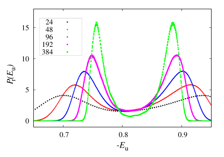
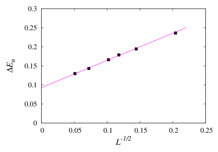
Figure 3: (Color online) Reweighted probability distribution $P_{\rm r}(E_{\rm u})$, and the distance between the two-peak positions $\Delta E_{\rm u}$ for $K_{1}^{\rm I}=0.8$. The height of the peaks increases with system size.

In the case of a first-order transition, we also expect metastable phases in a temperature range about the self-dual point, with lifetimes that are much larger than the time scale describing the jump from a metastable to a stable branch. We checked for such hysteresis in the model with $K_{1}/K_{2}=5$ by simulations sweeping slowly over ranges of couplings including the self-dual point. To find clear hysteresis loops, one has to simulate rather large systems. Results for $L=576$, with data points representing simulations of a half million Metropolis sweeps, separated by steps of $10^{-4}$ times the self-dual coupling, are shown in Fig. 4. The hysteresis loop covers only $10^{-3}$ of the $K/K_{\rm sd}$ scale, where $K_{\rm sd}$ denotes the self-dual couplings.

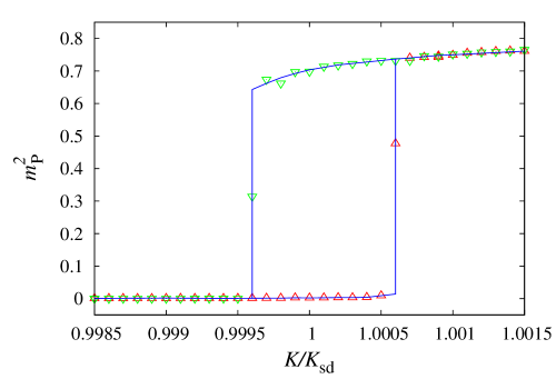
Figure 4: (Color online) Hysteresis loop for the squared magnetization $m_{\rm P}^{2}$ of an $L=576$ system with $K_{1}/K_{2}=5$. The horizontal scale shows the couplings in units of the self-dual couplings for this ratio. Each data point represents a simulation of $5\times 10^{5}$ Metropolis sweeps. The results for increasing couplings are shown as $\bigtriangleup$, for decreasing couplings as $\bigtriangledown$. The lines are added for visual aid only.

V Results for $q>2$

V.1 Transfer-matrix calculations

We have constructed transfer-matrix algorithms for the $q=3$ and 4 generalization of the Baxter-Wu model with $K_{1}=K_{2}$. The program is rather similar to that for the Baxter-Wu model, the main difference is that we have to use ternary or quaternary numbers to characterize a row of site variables, instead of binary numbers. As a consequence, a smaller range of system sizes can be handled. The finite-size data are here restricted to $L\leq 18$ for $q=3$ and $L\leq 12$ for $q=4$.

We computed the largest eigenvalue of the transfer matrix, as well as the magnetic eigenvalue, characterized by the antisymmetry under a lattice reflection of the corresponding eigenstate. Next, the correlation length and the scaled gap were obtained from Eqs. (22) and (23). The results for the scaled gap are shown in Table 2.

Table 2: Results of transfer-matrix calculations of the scaled magnetic gaps for the $q=3$ and 4 generalized Baxter-Wu models, at the respective self-dual points with $K_{1}=K_{2}$. The columns under ”$p$” show the exponent obtained from the three-point fits described in the text.

	$q=3$		$q=4$
$L$	$X_{h}(L)$	$p$	$X_{h}(L)$	$p$
3	0.129163		0.13050
6	0.117738	1.19	0.10381	1.04
9	0.105105	0.71	0.07655	0.37
12	0.093650	0.62	0.05460
15	0.083255	0.54
18	0.073778

The behavior of the scaled gaps does not suggest convergence with increasing $L$. Three-point fits according to Eq. (28) yield positive values of the exponent $p$. This does not agree well with the description of the finite-size data in terms of an attractive critical fixed point. It rather suggests crossover to some other, sufficiently remote fixed point. That may well be a discontinuity fixed point NN . Both for $q=3$ and 4, the behavior of the scaled gaps as a function of $L$ is similar to that found in Sec. IV.1 at intermediate values of $K^{\rm I}_{1}$.

Transfer-matrix calculations at couplings with $K_{1}=K_{2}$ in the vicinity of the self-dual value show clear signs of transitions. The scaled magnetic gaps shown in Figs. 5 and 6 for $q=3$ and 4 respectively, display the same type of transition behavior as found ins Sec. IV.1 for a $q=2$ model: for couplings exceeding the self-dual value the scaled gaps tend to zero, and at the high-temperature side the scaled gaps are increasing with system size.

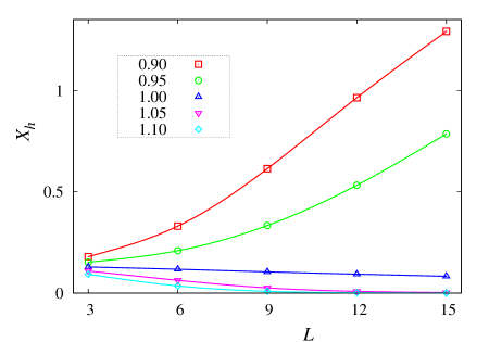
Figure 5: (Color online) Scaled gaps of the $q=3$ generalized Baxter-Wu model as a function of system size $L$, for five different couplings in the vicinity of the self-dual point. From top to bottom, the data apply to 0.9, 0.95, 1, 1.05, and 1.1 times the self-dual coupling. These data suggest that a phase transition takes place near the self-dual point.

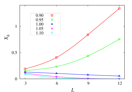
Figure 6: (Color online) Scaled gaps of the $q=4$ generalized Baxter-Wu model as a function of system size $L$, for five different couplings in the vicinity of the self-dual point. From top to bottom, the data apply to 0.9, 0.95, 1, 1.05, and 1.1 times the self-dual coupling. These results are similar to those for the $q=3$ model, but the gap at the self-dual point decays more rapidly with $L$ for $q=4$.

V.2 Monte Carlo results

Also in this case we employ Monte Carlo simulations to obtain independent and additional evidence about the character of the phase transitions. In addition to the evidence already reported by Alcaraz et al. AJ ; ACO , it remains to be investigated whether hysteresis is present, and whether one can extrapolate the energy discontinuity to the thermodynamic limit.

We employed the Metropolis method as well as the cluster algorithm defined in Sec. III.2. However, in the present case $q>2$, the efficiency of the cluster method is not much different from that of the Metropolis algorithm.

We first simulated the $K_{1}=K_{2}$ self-dual point of the $q=3$ model, and sampled the energy distribution for a number of system sizes that are multiples of 3. The energy $E$ is defined as minus the density of satisfied triangles per site. Again the distribution has two unequal peaks, but their separation is wider than in the $q=2$ case. The reweighting was done by multiplication of the histogram with $e^{a+bE}$. The reweighted distribution $P_{\rm r}(E)$ is shown in Fig. 7 for several system sizes.

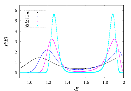
Figure 7: (Color online) Reweighted probability distribution $P_{\rm r}(E)$ for the $q=3$ model. Data are shown for system sizes $L=6$, 12, 24 and 48. Data points for the same system size are connected by a curve for the purpose of clarity. The heights of the peaks increase with system size.

The local minimum between the peaks decreases as a function of $L$. In the range of finite sizes covered by our simulations, the distance between the peaks approaches a nonzero constant approximately as $1/L$, as shown in Fig. 8. Such behavior was also found by Lee and Kosterlitz LK for the first-order transition of the $q>4$ Potts model. The average of the two peaks, also shown in this figure, extrapolates within numerical uncertainty to the value $1+1/\sqrt{3}$ predicted by self-duality.

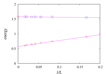
Figure 8: (Color online) Distance along the energy scale between the peaks ($\bigtriangleup$), and minus the mean of the peaks ($\square$) of the energy histogram of the $q=3$ model versus inverse system size. Duality predicts the mean of the peaks at the position marked by _○.

Next, we performed similar simulations of the $q=4$ model at the self-dual point. The reweighted probability distribution $P_{\rm r}(E)$ is shown in in Fig. 9 for several system sizes.

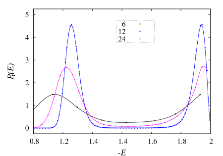
Figure 9: (Color online) Reweighted probability distribution $P_{\rm r}(E)$ for the $q=4$ model. Data are shown for system sizes $L=6$, 12 and 24. Data points for the same system size are connected by a curve for the purpose of clarity. The height of the peaks increases with system size.

The distances between the maxima of the histogram are shown in Fig. 10 as a function of the inverse system size. They extrapolate to a nonzero constant. The average peak positions, also shown in Fig. 8, agree well with the value $3/2$ predicted by duality.

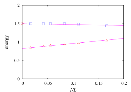
Figure 10: (Color online) Distance along the energy scale between the peaks ($\bigtriangleup$), and minus the mean of the peaks ($\square$) of the energy histogram of the $q=4$ model versus inverse system size. Duality predicts the mean of the peaks at the position marked by _○.

Also these data agree with the expectations for a first-order transition, and even more strongly so than in the $q=3$ case, for instance, because the distances between the peaks of the energy histograms are larger.

To test for the presence of hysteresis, we performed Monte Carlo simulations of the $q=3$ and 4 models, varying the temperature in a region close to the symmetric self-dual point. Each data point involved a simulation of $2\times 10^{5}$ Metropolis sweeps, of which the first $10^{4}$ were used for equilibration. The results for the magnetization-type quantity $m^{2}_{\rm P}$ are shown in Figs. 11 and Fig. 12. They display a small hysteresis loop for $q=3$, covering only a half percent of the $K$ scale, and stronger hysteresis effects for $q=4$.

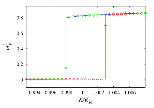
Figure 11: (Color online) Hysteresis loop of the magnetization-like quantity $m^{2}_{\rm P}$ for the $q=3$ model with size $60^{2}$. The horizontal scale shows the coupling in units of the self-dual coupling. The results for increasing couplings are shown as $\bigtriangleup$, for decreasing couplings as $\bigtriangledown$. The lines are added for visual aid only.

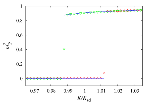
Figure 12: Hysteresis loop of the magnetization-like quantity $m^{2}_{\rm P}$ for the $q=4$ model with size $60^{2}$. The horizontal scale shows the couplings in units of the self-dual coupling. The results for increasing couplings are shown as $\bigtriangleup$, for decreasing couplings as $\bigtriangledown$. The lines are added for visual aid only.

VI Conclusion

The numerical results presented in Sec. IV.1 for the Baxter-Wu model ($q=2$, $K_{1}=K_{2}$) clearly converge to the known exact values $X_{t}=1/2$ and $X_{h}=1/8$. For $K_{1}\neq K_{2}$ deviations from this behavior are observed, and the dependence of these estimates on the finite size $L$ is considerable when $K_{1}$ and $K_{2}$ are sufficiently different. At first sight, this situation may seem similar to the poor convergence observed for some models in the 4-state Potts universality class, see e.g. Ref. BN1982 .

However, there are also significant differences. First we note that, except for ratios $K_{1}/K_{2}$ close to 1, the differences in the finite-size estimates for $X_{t}$ and $X_{h}$ tend to increase with increasing system size. Second, the finite-size estimates for $X_{t}$ and $X_{h}$ are smaller than the exact values for the Baxter-Wu model, instead of larger as observed for the $q=4$ Potts model BN1982 ; NB83 .

The interpretation of these observations is suggested by the renormalization flow diagram for the surface of phase transitions of the dilute two-dimensional Potts model proposed by Nienhuis et al. NBRS . The parameter space of that work involved the chemical potential $v$ of vacant sites and the number of Potts states $q$. The mapping of the Potts model onto the random-cluster model KF enables one to treat $q$ as a continuous variable. Since vacant sites in the Potts model are dual to multisite interactions Yolanda , the parameter $v$ may as well be interpreted as a scaling field depending on the type of interactions. At $q=4$, the field $v$ becomes marginal NBRS at the critical point.

We reproduce this flow diagram NBRS , adapted to our purposes, in Fig. 13. The $q=4$ Potts model is located at a value of $v$ smaller than that at the $q=4$ fixed point, and is still attracted by it, although marginally. This explains the slow finite-size convergence, and the logarithmic factors of the $q=4$ Potts model. The Baxter-Wu model is located at the $q=4$ fixed point.

The introduction of a difference between $K^{\rm I}_{1}$ and $K^{\rm I}_{2}$, such that the condition of self-duality is still satisfied, allows for the possibility that the location of the model in Fig. 13 changes. The coordinate $q$ will remain unchanged, but a priori there does not seem to be a way to tell whether the model will move up or down in the diagram, or perhaps will keep its location. But, since the finite-size estimates of $X_{h}$ and $X_{t}$ for the $K^{\rm I}_{1}\neq K^{\rm I}_{2}$ models and those for the $q=4$ Potts model lie on opposite sides with respect to the Baxter-Wu model, we may locate the $K^{\rm I}_{1}\neq K^{\rm I}_{2}$ models at a value of $v$ exceeding that of the Baxter-Wu model, as indicated by “2C” in Fig. 13. Therefore they flow to the discontinuity fixed point NN located at large $v$, so that the phase transition is discontinuous. In view of the symmetry between $K_{1}$ and $K_{2}$, the marginally relevant field $v$ can, in lowest order, not depend linearly on $K_{1}-K_{2}$ near the 4-state Potts fixed point, and one expects a contribution as $(K^{\rm I}_{1}-K^{\rm I}_{2})^{2}$. This is consistent with the very weak dependence of the finite-size data in Table 1 on small differences $K^{\rm I}_{1}-K^{\rm I}_{2}$.

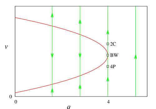
Figure 13: (Color online) Renormalization flow in the plane of phase transitions of the dilute random-cluster model, parametrized by the number of Potts states $q$ and the fugacity $v$ of vacancies, according to Ref. NBRS . The curve represents a line of fixed points. Its lower branch is attractive and describes the critical random-cluster model. The upper branch of fixed points is repulsive and describes the tricritical random-cluster model. When $v$ exceeds its tricritical value, the renormalization flow leads to a discontinuity fixed point, corresponding with a first-order transition. The position of the Baxter-Wu model (BW), of the $q=4$ Potts model (4P) and the presently investigated self-dual $q=2$ models with $K_{1}\neq K_{2}$ (2C) are sketched.

Thus we conclude that the generalized Baxter-Wu model with different couplings described by the Hamiltonian (2) undergoes a phase transition at the self-dual line for $q\geq 2$, and that the phase transition is first order for $K_{1}\neq K_{2}$, although extremely weakly so when the difference $K_{1}-K_{2}$ is small. Even for a rather large difference $K_{1}/K_{2}=5$, we find (see Fig. 4) a very narrow hysteresis loop.

Furthermore, for $q=3$ and 4 the transition is also discontinuous. This result disproves the possibility mentioned in Sec. I that the $q>2$ self-dual generalized Baxter-Wu models renormalize to a Coulomb gas in which the fugacity of the electric charges vanishes, in which case algebraic critical behavior would occur. Apparently the fugacity is nonzero, and, since the electric charges are relevant for $q>2$, the models renormalize away from the Gaussian line to a discontinuity fixed point.

The first-order character of the $q=4$ model, as expressed, for instance, by the energy discontinuity, is stronger than that of the $q=3$ model. We expect the first-order character to grow even stronger with a further increase of $q$ and/or the introduction of an asymmetry $K_{1}\neq K_{2}$.

Acknowledgement: This research is supported by the NSFC under Grant No. 10675021, and by the HSCC (High Performance Scientific Computing Center) of the Beijing Normal University, and, in part, by the Science Foundation of the Chinese Academy of Sciences. HB thanks the Beijing Normal University and the University of Science and Technology of China in Hefei for hospitality extended to him. W. G. acknowledges hospitality extended to him by the Lorentz Institute.

References

- (1) B. Nienhuis, A. N. Berker, E. K. Riedel and M. Schick, Phys. Rev. Lett. 43, 737 (1979).
- (2) M. Nauenberg and D. J. Scalapino, Phys. Rev. Lett. 44, 837 (1980).
- (3) R. J. Baxter and F. Y. Wu, Phys. Rev. Lett. 31, 1294 (1973); Aust. J. Phys. 27, 357 (1974).
- (4) G. T. Barkema, M. E. J. Newman, and M. Breeman, Phys. Rev. B 50, 7946 (1994).
- (5) R. B. Potts, Proc. Cambridge Philos. Soc. 48, 106 (1952).
- (6) B. Nienhuis, in Phase Transitions and Critical Phenomena, edited by C. Domb and J. L. Lebowitz. (Academic Press, London, 1987), Vol. 11, p. 1, and references therein.
- (7) F. C. Alcaraz and L. Jacobs, Nucl. Phys. B 210 [FS6], 246 (1982).
- (8) F. C. Alcaraz, J. L. Cardy and S. O. Ostlund, J. Phys. A. 16, 159 (1983).
- (9) H. A. Kramers and G. H. Wannier, Phys. Rev. 60, 252 (1941).
- (10) C. Gruber, A. Hintermann and D. Merlini, Group Analysis of Classical Lattice Systems (Springer, Berlin 1977).
- (11) L. Turban, J. Phys. C 15, L227 (1982).
- (12) G-M. Zhang and C-Z. Yang, J. Phys. A 26, 4907 (1993).
- (13) H. W. J. Blöte, J. R. Heringa and A. Hoogland, Phys. Rev. Lett. 63, 1546 (1989).
- (14) M. P. Nightingale, Proc. K. Ned. Akad. Wet., Ser. B (Palaeontol., Geol., Phys., Chem.) 82, 235 (1979).
- (15) H. W. J. Blöte and M. P. Nightingale, Physica A (Amsterdam) 112, 405 (1982).
- (16) X.-F. Qian, M. Wegewijs and H. W. J. Blöte, Phys. Rev. E 69, 036127 (2004).
- (17) J. L. Cardy, J. Phys. A 17, L385 (1984).
- (18) For reviews, see e.g. M. P. Nightingale in Finite-Size Scaling and Numerical Simulation of Statistical Systems, ed. V. Privman (World Scientific, Singapore 1990), and M. N. Barber in Phase Transitions and Critical Phenomena, eds. C. Domb and J. L. Lebowitz (Academic, New York 1983), Vol. 8.
- (19) M. A. Novotny and H. G. Evertz in Computer simulation studies in condensed-matter physics VI, edited by D. P. Landau, K. K. Mon and H.-B. Schüttler (Springer, Berlin 1993), 188.
- (20) X.-J. Li and A. D. Sokal, Phys. Rev. Lett. 63, 827 (1989).
- (21) Y. Deng, J. Salas and and A. D. Sokal, unpublished (2009).
- (22) J. Lee and J. M. Kosterlitz, Phys. Rev. B 43, 3265 (1991).
- (23) B. Nienhuis and M. Nauenberg, Phys. Rev. Lett. 35, 477 (1975).
- (24) A. M. Ferrenberg and R. H. Swendsen, Phys. Rev. Lett. 61, 2635 (1988).
- (25) M. P. Nightingale and H. W. J. Blöte, J. Phys. A 16, L657 (1983).
- (26) P. W. Kasteleyn and C. M. Fortuin, J. Phys. Soc. Jpn. 46 (Suppl.), 11 (1969); C. M. Fortuin and P. W. Kasteleyn, Physica (Amsterdam) 57, 536 (1972).
- (27) Y. M. M. Knops, H. W. J. Blöte and B. Nienhuis, J. Phys. A 26, 495 (1993).