Radiative transfer models of mid-infrared H₂O lines in the Planet-forming Region of Circumstellar Disks

Abstract

The study of warm molecular gas in the inner regions of protoplanetary disks is of key importance for the study of planet formation and especially for the transport of H₂O and organic molecules to the surfaces of rocky planets/satellites. Recent Spitzer observations have shown that the mid-infrared spectra of protoplanetary disks are covered in emission lines due to water and other molecules. Here, we present a non-LTE 2D radiative transfer model of water lines in the 10-36 $\mu$m range that can be used to constrain the abundance structure of water vapor, given an observed spectrum, and show that an assumption of local thermodynamic equilibrium (LTE) does not accurately estimate the physical conditions of the water vapor emission zones, including temperatures and abundance structures. By applying the model to published Spitzer spectra we find that: 1) most water lines are subthermally excited, 2) the gas-to-dust ratio must be as much as one to two orders of magnitude higher than the canonical interstellar medium ratio of 100-200, and 3) the gas temperature must be significantly higher than the dust temperature, in agreement with detailed heating/cooling models, and 4) the water vapor abundance in the disk surface must be significantly truncated beyond $\sim 1~{}$AU. A low efficiency of water formation below $\sim 300\,$K may naturally result in a lower water abundance beyond a certain radius. However, we find that chemistry, although not necessarily ruled out, may not be sufficient to produce a sharp abundance drop of many orders of magnitude and speculate that the depletion may also be caused by vertical turbulent diffusion of water vapor from the superheated surface to regions below the snow line, where the water can freeze out and be transported to the midplane as part of the general dust settling. Such a vertical cold finger effect is likely to be efficient due to the lack of a replenishment mechanism of large, water-ice coated dust grains to the disk surface.

1. Introduction

Planets are thought to predominantly form within 10 AU of young low mass stars ($<$ a few solar masses). Concurrent with the process of planet formation, a rich carbon, nitrogen and oxygen chemistry evolves to eventually form the building blocks of the icy bodies within young planetary systems; moons around giant planets, comets and Kuiper belt objects. This chemistry will also seed the surfaces of rocky terrestrial planets with water and organics, probably either through impacts with comets or carried in hydrated refractory meteorites (Raymond et al., 2004).

This early, highly active and evolving stage takes place within the first few million years of a star’s lifetime while the protoplanetary disk is still gas-rich. The planet forming region can therefore be traced by observations of warm (100-2000 K) molecular gas, through a multitude of rotational and rovibrational transitions spanning the infrared wavelength range (2-200 $\mu$m).

One critical question is how the distribution of water occurred in the Solar Nebula and how the surface of the young Earth was hydrated. Salyk et al. (2008) and Carr & Najita (2008) report detections of hundreds of water vapor lines in three protoplanetary disks observed with the Spitzer Space Telescope InfraRed Spectrometer (IRS) between 10 and 36 $\mu$m. These first, pioneering spectra were analyzed using simple ‘slab models’ that assume level populations consistent with thermodynamic equilibrium and otherwise consisting only of a column density, a single excitation temperature and an emitting solid angle.

Fits to data using such simple slab models result in column densities of $N_{\rm CO}=6-7\times 10^{18}$ cm^-2, $N_{\rm H_{2}O}=6-8\times 10^{17}$ cm^-2, and $N_{\rm OH}=2\times 10^{17}$ cm^-2 and an excitation temperature $T=1000$ K for DR Tau and AS 205A, which is similar to the observations of AA Tau by Carr & Najita (2008). The latter paper also reports the detection of CO₂ and that of the small organics C₂H₂ and HCN. Given a slab model, the line emission is derived to be confined within radii ranging from 0.6 to 3.0 AU.

Recently, a number of theoretical models have appeared that focus on the gas-phase thermo-chemical modeling of the inner regions of protoplanetary disks (Markwick et al., 2002; Glassgold et al., 2004; Nomura & Millar, 2005; Nomura et al., 2007; Agúndez et al., 2008; Gorti & Hollenbach, 2008; Ercolano et al., 2008; Woods & Willacy, 2009; Glassgold et al., 2009; Woitke et al., 2009). These papers have different levels of complexity in their adopted physics (e.g., treatment of X-rays and/or FUV, the possibility of transport throughout the disk, time-dependent treatment of chemistry) and deal with various chemical aspects (e.g., organic species, H₂O, carbon fractionation). Other theoretical models focus on the dynamical transport of individual species through the disk (Stevenson & Lunine, 1988; Ciesla & Cuzzi, 2006; Ciesla, 2009). A key question is therefore whether the large amounts of warm ($T\sim 300-1000$ K) water that have been observed can be explained by models with either in situ formation or dynamical transport from larger radii.

To date, neither the observational work nor the theoretical papers that consider the chemistry in the inner region of protoplanetary disks have shown how physical parameters – specifically the actual abundance structure of a given molecule – can be derived from line observations in a meaningful way. In this paper, we propose that, given the complexity of inner disk chemistry and volatile dynamics, progress can best be made by separating the chemical-dynamical model from the radiative transfer modeling of observations. This way, high quality observations, such as infrared imaging spectroscopy, can be used to derive an abundance structure of a given molecule by application of a radiative transfer code that performs: 1) a non-LTE excitation calculation in a disk-geometry followed by, 2) raytracing that correctly samples the velocity field at small radii, and 3) a front end that simulates the action of the appropriate telescope/instrument. Given a derived abundance structure, the interpretation step, using chemical-dynamical models, becomes much easier than the approach in which one begins with the chemical model. This paper describes step 1). A companion paper describes steps 2) and 3) (Pontoppidan et al., 2009).

Here our major focus is an examination of the excitation and infrared radiative transfer of water vapor in the surface layers of protoplanetary disk. We find that water vapor must be strongly depleted from the surface over a significant range of radii. This can be due to a chemical effect, as water is less efficiently formed at temperatures $T<300$ K (Glassgold et al., 2009); but we speculate that additional depletion is active due to vertical gas diffusion, followed by freeze-out below the snow line and settling to the mid-plane on icy dust grains. This process is analogous to the radial cold finger effect proposed by Stevenson & Lunine (1988), but will not be balanced by the inward radial migration of icy bodies (Salyk et al., 2008). To distinguish it from the radial cold finger effect, we call it the vertical cold finger effect (see Section 5.2).

To place the non-LTE model into context, we first describe slab models of disk infrared emission and the collisional/radiative excitation of water. The details of the statistical equilibrium calculations are then presented, along with our initial results and general conclusions. The models presented here are meant only to provide a fundamental analysis of the global properties of water vapor emission from disks, the more elaborate parameter study of the water excitation model that is needed to fit the Spitzer IRS spectra of individual sources is postponed to a separate paper (Meijerink et al. 2009, in preparation).

2. LTE slab models versus non-LTE 2D models

Recent papers from Salyk et al. (2008) and Carr & Najita (2008) have been successful in obtaining good matches to H₂O line observations in the Mid-Infrared (MIR) Spitzer-IRS band ($\lambda\sim 10-36\mu$m) using single temperature, single column density LTE models with no global kinematics, such as Keplerian motion. These fits have been used to provide numerical estimates of the warm water column densities. Since a key point of this work is to show why non-LTE calculations are required to quantitatively interpret the observed molecular line spectra of the warm inner regions of protoplanetary disks, particularly the emission from H₂O, we first examine the successes and limitations of LTE ‘slab’ models. We will argue below that taking the properties derived from such models at face value is dangerous and may well lead to erroneous conclusions when attempting to compare abundances with chemical models. Specifically, a good fit in a given wavelength range does not imply that the fitting model is correct. The low resolution of the Spitzer spectra, and the resulting lack of line profile information, introduce significant degeneracies, as we discuss next. We will then show that the introduction of relatively simple physics lead to constraints not available from slab models, and that a requirement to match all lines in the observed Spitzer range can significantly constrain the results. Although the lineshapes also contain a great deal of info, it is not considered here, since the IRS has a resolution of $R=\lambda/\Delta\lambda=600$ (500 km/s).

Slab models ignore the complex geometric structure of protoplanetary disks. In the inner regions, densities can be as high as $n_{\rm H}>10^{16}$ cm^-3 in the midplane and at small radii ($R<0.5$ AU), but decrease with radius and height (see Fig. 4) over many orders of magnitude to densities $n<10^{3}$ cm^-3. Gas temperatures can be as high as $T\sim 5000~{}K$ in the upper reaches of the disk atmosphere where the X-ray (Glassgold et al., 2004) or FUV (Kamp & Dullemond, 2004) attenuation is minimal. The temperature drops steadily in the shielded regions of the disk to values of $T\sim 10-100$ K, where the gas temperature couples strongly to the dust temperature. Therefore, the disk consists of an ensemble of densities and temperatures. Lines are, in general, the result of emission from a range of disk radii, and thus cannot be represented by a single excitation temperature. The mid-infrared wavelength region contains radiative transitions from upper levels with an enormous range of energies, from values at/near the photon energy ($E<720$ K or 500 cm^-1) to values in excess of $E>7200$ K or 5000 cm^-1. The conversion between wavenumber and temperature units is 1.44. Temperature units are used throughout this paper. For a light, asymmetric top molecule, such as H₂O, transitions with various upper state energies can be highly scattered throughout the spectrum, and even a small spectral region can contain lines that trace very different regions of the disk. Therefore, the assumption that all lines are formed in the same region of the disk is immediately seen to be inappropriate – and can easily lead to an erroneous determination of the line optical depth in a slab model. In fact, it is essentially meaningless to even assign an optical depth to a given line, since emission from different disk radii will have local optical depths varying by orders of magnitude.

Furthermore, LTE assumes that the level populations are in accordance with the Maxwell-Boltzmann distribution at a particular temperature. This only holds when collisions dominate the molecular excitation/relaxation, or numerically when the ambient densities are higher than the critical densities $n_{crit}=A_{ul}/C_{ul}$, where $A_{ul}$ and $C_{ul}$ are the radiative and collisional decay rates of a particular transition. The critical densities for the excitation of the water lines through collisions range between $n_{crit}=10^{8}$ to $>10^{12}$ cm^-3, and tend to increase strongly with excitation energy. Pure rotational transitions with low excitation energies, which lie in the frequency range of the Heterodyne Instrument for the Far-Infrared (HIFI) on the Herschel Space Observatory (Herschel), have critical densities in the range $10^{8}-10^{9}$ cm^-2. Unfortunately, these lines will likely be difficult to observe toward disks with HIFI for sensitivity reasons (Meijerink et al., 2008). Spitzer-IRS ($10-36$ $\mu$m range) data, on the contrary, have shown rich spectra of warm water in the inner regions of protoplanetary disks. These consist of rotational transitions with even larger critical densities than the HIFI lines and are therefore unlikely to be thermalized. Lower excitation lines of a given species tend to have lower critical densities, and as a result, lines with lower excitation energies will trace larger regions of the disk. It is therefore expected that the line shapes and line images will differ significantly from one transition to another. Thus, future spectrally and spatially resolved data will be crucial for constraining the water abundance structure, and should be interpreted with tools that specifically model (or mimic) the physical and chemical properties of the disk.

3. Excitation of H₂O

There are a number of ways to excite water to higher energy states: 1) collisions with, e.g., H, H₂, He, and electrons; 2) excitation by radiation produced by hot dust located at the inner rim of the disk; 3) photo-desorption from dust grains; and 4) chemical formation in highly excited states. In this paper, we only take into account 1) and 2). For this study all hydrogen is assumed to be in molecular form, and He excitation is considered by scaling the molecular hydrogen rates. Electron excitation is neglected, since electrons are expected to be abundant only in unshielded low density regions, where water is subthermally excited and its fractional abundance very low, which therefore do not contribute much to the overall line emission.

Water lines in the $10-36~{}\mu$m wavelength range covered by the Spitzer-IRS Short-High (SH) and Long-High (LH) modules are overwhelmingly dominated by pure rotational transitions between levels in the ground ($v_{1}v_{2}v_{3}$)=(000) vibrational state as well as between those in the first vibrational state ($v_{1}v_{2}v_{3}$)=(010). Further, for a non-LTE calculation, transitions that connect the two vibrational levels must also be considered.

Given the widespread importance of water, there have been significant efforts to calculate the H₂O excitation rates – both experimentally and theoretically. Unfortunately, most studies only give state-to-state rate coefficients below the first excited vibrational level, i.e, below $E=2294.4$ K (Green et al., 1993; Phillips et al., 1996; Faure et al., 2004, 2007; Dubernet & Grosjean, 2002; Grosjean et al., 2003). The only H₂O-H₂ and H₂O-electron collisional rates for higher levels of excitation currently available are from Faure & Josselin (2008). This database contains all collisional rotational and ro-vibrational transitions between the 5 lower vibrational levels, ($v_{1}v_{2}v_{3}$)=(000), (010), (020), (100), and (001), up to an energy $E=7200$ K. The authors expect the data to be accurate within a factor of $\sim 5$ for the largest rates ($\geq 10^{-11}$ cm³ s^-1). Smaller rates, which also include the rovibrational excitation/de-excitation, are expected to be accurate to an order of magnitude. Summed rates and cooling rates have better precision and the data are well suited for the modeling of emission spectra.

In Fig. 1, the intensities for lines at $T=700$ K are shown, selected to be in the Spitzer-IRS spectral range between 10 and 36 $\mu$m. The top panel shows the intensity of all lines in the HITRAN database (Rothman et al., 2005), where the lines with upper level energy $E\leq 7194$ K are the open green circles ($n=1454$), and the lines with $E>7194$ K in red filled circles ($n=142$). Because collisional rates between levels with energy $E>7194$ K are not available it is possible that potentially strong lines are not calculated, especially in the 10 - 15 $\mu$m spectral range. Therefore, the calculation of these rates is important for future modeling.

To limit the computational load, the non-LTE calculation is restricted to transitions in the ($v_{1}v_{2}v_{3}$)=(000) and (010) vibrational levels. In the lower panel in Fig. 1 we show the intensity of transitions with upper level energy $E\leq 7200$ K, where the transitions between levels in the ($v_{1}v_{2}v_{3}$)=(000) and (010) are in green open circles ($n=1230$) and all others ($n=224$) are in red filled circles. It can be seen that the excluded vibrational levels contain lines that are weaker by 1-2 orders of magnitude relative to lines in the vibrational levels modeled. At the Spitzer-IRS SH+LH spectral resolution of R=600, these lines are unlikely to contribute significantly to the overall spectrum.

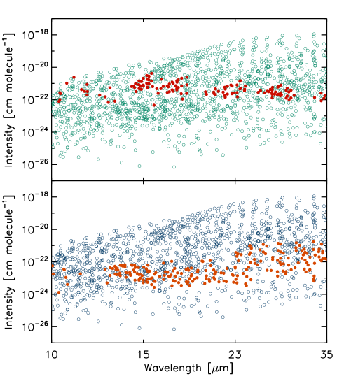
Figure 1.— LTE intensities at $T=700$ K for: (top) Lines with upper level energy $E\leq 7194$ K (open green circles) and upper level energy $E>7194$ K (filled red circles); (bottom) Lines with lower and upper level in v=000 or v=010 (open blue circles) and all other transition (orange filled circles) both with upper level energy $E\leq 7194$ K.

4. Model setup

Next we investigate how the H₂O 10 - 36 $\mu$m spectrum depends on the properties of the disk. The aim is to derive a fiducial model that qualitatively matches the observed data. Quantitative fits to the spectra of individual sources are postponed to a later paper. The central star is chosen to be a representative T Tauri. It has mass $M=1.0$ M_⊙, age $t=2$ Myrs, and solar metallicity $Z=0.02$, corresponding to a radius $R=2.0$ R_⊙ and effective temperature $T_{\rm eff}=4275$ K when using the pre-main sequence tracks of Siess et al. (2000). The stellar spectrum is a Kurucz stellar model (Kurucz, 1993). An inclination of $30^{\circ}$ is adopted for rendering of spectra.

The disk has a mass of $M=0.01$ M_⊙, outer radius $R_{\rm out}=120$ AU, flaring parameter $H/R\propto R^{2/21}$, and outer pressure scale height $h_{p}/R=0.10$. These parameters determine how much light is intercepted at each radius and thus the temperature distribution of the disk. We adopt a Gaussian density distribution in the vertical direction and a radial surface density $\Sigma\propto R^{-1}$. The disk is roughly in hydrostatic equilibrium (for an isothermal disk), but flatter than the Chiang & Goldreich (1997) disk ($H/R\propto R^{2/7}$), giving us a better correspondence to the observed spectral energy distributions in our sample of T Tauri disks. However, we emphasize that the model is not an attempt to fit any particular disk. The dust sublimation temperature is set at $T\sim 1600$ K, giving a radius of the inner rim of $R_{rim}=0.075$ AU.

In addition to parameters determining the dust structure of the disk, a number of parameters are needed for the line modeling. These are the prescription of the intrinsic line width, the freeze-out model, the fractional H₂O abundance and the gas temperature and density structure. We assume that the intrinsic linewidth throughout the grid is determined by thermal broadening ($v_{th}=\sqrt{2kT/\mu_{\rm H2O}m_{p}}$), and turbulent broadening, assumed to be a fraction of the sound speed $v_{turb}=\epsilon c_{s}$, where $\epsilon=0.03$ is adopted in this paper. The intrinsic linewidth is therefore dominated by thermal broadening. Five different model types are considered: 1) Constant water abundance throughout the disk; 2) Reduced water abundance in regions where water freezes out (see Fig. 3); 3) Decoupling of gas temperature and destruction of water where gas is exposed to direct stellar irradiation; 4) Increasing the gas-to-dust ratio from 1280 (which is already and order of magnitude beyond the standard interstellar medium value) to 12800, and 5) Truncation of the water abundance beyond $R\sim 1$ AU due to the vertical cold finger effect. The model parameters are summarized in Table 1.

Table 1Model input

Parameter	Computational range
$v_{turb}=\epsilon c_{s}$ [km/s]	$<0.01-0.05$
$v_{th}=\sqrt{\frac{2kT}{\mu_{H_{2}O}m_{p}}}$ [km/s]	0.1 - 2.0 (T=10-5000 K)
$x({\rm H_{2}O})$	$10^{-10}-3\times 10^{-4}$
$T_{freeze}$	$100-200$ K (see Fig. 3)
$H/R\propto R^{\alpha}$	$\alpha=2/21$
$h_{p}/R$ (R=120 AU)	0.10
$M_{*}$ [M⊙]	$1.0$
$R_{*}$ [R⊙]	$2.0$
$T_{eff}$ [K]	$4275$
opacities	see Fig. 2
gas-to-dust ratio	1280 (1-3); 12800 (4-5)
disk inclination	$30^{\circ}$

The water emission spectrum is calculated as follows:

(i) First, the dust temperature distribution and the mean intensity in the disk is determined using the 2D dust radiation transfer code RADMC (Dullemond & Dominik, 2004). The mean intensity is used to calculate the radiative (de-)excitation rates $B_{ij}<J_{ij}>$. The adopted dust mixture contains 15 percent carbon grains and 85 percent silicate grains. The two dust components are thermally coupled. The dust mass distribution and opacities are shown in Fig. 2. The silicate dust size distribution has a peak at $1-10~{}\mu$m grains, while the carbon grains consists of both small and very large grains ($>10~{}\mu$m). This corresponds to grains that have grown beyond those found in the interstellar medium (Kessler-Silacci et al., 2006). It is implicitly assumed that grains larger than 40 $\mu$m have settled to the midplane where they do not affect the water lines (which are formed near the disk surface).

Figure 2.— Dust size distribution with minimum grainsize $a_{min}=3\times 10^{-4}$ $\mu$m and maximum grainsize $a_{max}=40$ $\mu$m and opacities of the silicate (solid) and carbonaceous grains (dashed). Most of the silicate grain mass is in the larger grains ($R=0.5-20\mu$m), while the carbonaceous grains have substantial reservoirs in both in small ($R<0.01\mu$m) and large grains ($R>1\mu$m).

(ii) The level populations are calculated with the radiative excitation code $\beta$3D (Poelman & Spaans, 2005, 2006), a multi-zone escape probability excitation code. It can be applied to arbitrary geometries and is suitable for any atom and molecule. This code is adopted because it is about 10-100 times faster than existing MC/ALI codes – especially when the lines are highly optically thick and IR pumped. While $\beta$3D can be used in 3 dimensional structures, it is only feasible in applications where a limited amount of levels ($\sim$10) are used. Here we adopt a 1+1D approximation to alleviate the computational expense of iterating over a total of $\sim 540$ levels for both ortho and para water, especially for a large grid of models. We calculate the excitation at a number of radial points ($\sim 100-120$), each of which is effectively treated as a separate 1D plane-parallel slab. The escape probability is therefore given by:

$$\beta(\tau)=\frac{1-\exp(-3\tau)}{3\tau},$$ (1)

where $\tau$ is the optical depth in the direction of the considered ray. The resulting vertical excitation structures are subsequently combined and regridded to polar coordinates, so that it can serve as input for the next step: raytracing with RADLite.

(iii) RADLite (described in a companion paper, Pontoppidan et al. 2009) is used to obtain the line spectra. It is a raytracer for axisymmetric geometries specifically set up to handle the large velocity gradients and small turbulent widths which are expected to be present in the planet-forming region of circumstellar disks.

To demonstrate how the model can be used to investigate the influence of different water abundance structures, two additional physical processes that determine the distribution of water vapor are included and described in the following sections.

4.1. Reduction of the water abundance due to freeze-out

Freeze-out of water onto grain surfaces can significantly reduce the amount of water in the gas phase, and will reduce the integrated line emission of the lower excitation lines (Meijerink et al., 2008). The approach from Pontoppidan (2006) is used to determine the pressure and dust temperature where the transition from water vapor to ice occurs on grains. The rate of ice mantle build-up is given by:

$$\frac{dn_{ice}}{dt}=R_{ads}-R_{des},$$ (2)

where $R_{des}=\nu_{0}\exp(-E/kT_{\rm dust})\times n_{\rm H_{2}O,ice}\times\gamma$ is the thermal desorption rate and $R_{ads}=n_{\rm H_{2}O}\times n_{dust}\times\pi d^{2}\times\sqrt{3kT_{\rm gas}/m_{\rm H_{2}O}}\times f$. The surface binding energy of $E=5773$ K is appropriate for water on a crystalline ice surface (Fraser et al., 2001). The desorption and adsorption rates depend on the dust and gas temperature, respectively, but freeze-out is only important where the gas is coupled to dust, i.e., $T_{\rm gas}=T_{\rm dust}$. Non-thermal desorption mechanisms are not included. $\gamma$ is a factor that takes into account the observation (in the laboratory) that H₂O only desorbs from the top monolayer (i.e., first order desorption for sub-monolayer coverage and zeroth order desorption for multilayers), $d=1$ $\mu$m is the average adopted grains radius, which is representative for that used by the radiative transfer models, although the precise choice does not affect the results, $f=1$ is the sticking coefficient, and $n_{\rm dust}$ and $n_{\rm H_{2}O}$ are dust and water number densities. The pre-exponential factor $\nu_{0}$ is expressed in s^-1 and is roughly the frequency of the vibrational stretching mode ($\lambda\sim$3.1 $\mu$m).

In Fig. 3, the density-dependent freeze-out temperature is shown. The system is assumed to have reached equilibrium, i.e., $dn_{ice}/dt=0$ – a reasonable assumption because the freeze-out timescales are short at the high densities in the disk surface ($n\gtrsim 10^{8}$ cm^-3). At lower densities, $n=10^{4}-10^{6}$ cm^-3, where equilibrium is not reached on time scales shorter than $10^{4-5}$ years and where photo-desorption occurs due to direct irradiation from the central star, dust temperatures are generally so high that freeze-out is not important. The freeze-out temperature is between $T=100-110$ K for dense ISM cloud conditions, $n=10^{4}-10^{6}$ cm^-3, and rises to temperatures as high as $T=150-180$ K for midplane densities in the inner region, $R=0.1-0.2$ AU, of the disk, $n=10^{12}-10^{14}$ cm^-3. If a region is below the freeze-out temperature, we adopt a residual gas phase abundance of $x_{\rm H_{2}O}=10^{-10}$ to simulate cosmic ray desorption.

Figure 3.— The density dependence of the freeze-out temperature of H₂O. Water is mostly frozen out for a give temperature and density left to the curve, and mostly in the gas phase when right to the curve

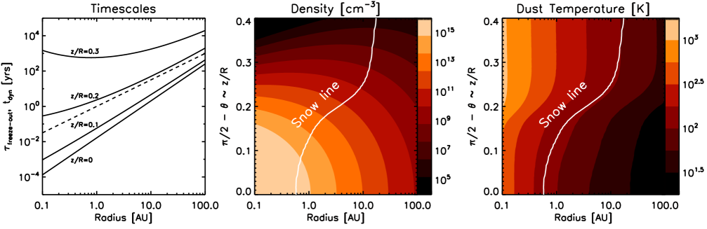
Figure 4.— Left: The e-folding timescales for freeze out are indicated by the black curves for selected scale heights in the disk. The Keplerian dynamical timescale is indicated by the dashed line for comparison. Middle: Gas total hydrogen number density. The snow-line is indicated as well. Right: Dust temperature.

4.2. Reduction of the H₂O abundance in the warm atmosphere

From static chemistry models (Glassgold et al., 2004; Kamp & Dullemond, 2004; Woitke et al., 2009) it is known that the gas and dust are kinetically uncoupled in the warm atmosphere of the disk where the ambient densities are in the range $n_{\rm H}=10^{4}-10^{9}$ cm^-3, leading to local gas temperatures that are significantly higher than that of the dust. The gas is at high temperatures ($T\sim 5000$ K) in the uppermost unshielded regions of the disk and drops to lower temperatures ($T\sim 100-200$ K) in deeper layers where the gas is coupled to the dust. If this transition zone contains water, it will have a strong effect on the line strengths of especially the high excitation lines. The gas/dust decoupling is associated with a reduced water abundance in the unshielded part of the disk due to photo-dissociation and ion-molecule reactions. A simple parametrized description is adopted here using the water abundance and temperature structure as shown in Fig. 2 at radius $R\sim 1$ AU of Glassgold et al. (2009). Warm water is present at temperatures $T\sim 300-1000$ K, but reduced by orders of magnitude at very high temperatures $T>2000$ K. The gas temperature and water abundance depend solely on the ionization parameter $\zeta/n_{\rm H}$, where $\zeta$ is the total ionization rate and $n_{\rm H}$ the number density of hydrogen. The ionization parameter is calculated assuming X-rays are the dominated radiation source. We adopt a thermal source with $T_{X}=1$ keV and $L_{X}=10^{29}$ erg/s. The total ionization rate for every point on the grid is calculated using the absorption cross sections from Morrison & McCammon (1983), and taking into account the attenuating column $N_{\rm H}$. For every 1 keV of energy absorbed, there are $1000/37\sim 27$ ionizations (see e.g. Glassgold et al. 1997 for more details). Using this prescription, it is possible to scale the Glassgold et al. (2009) results at $R=1$ AU to the entire disk given a local ionization parameter, and the resulting gas temperature is shown in Fig. 5. The adopted thermal and chemical profile can of course be affected by vertical mixing, but such considerations are beyond the scope of this paper.

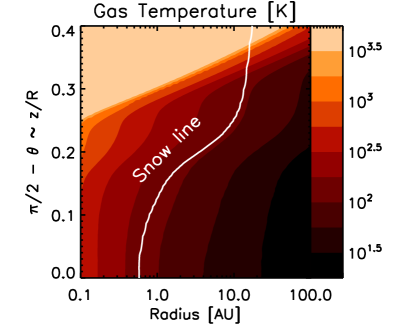
Figure 5.— Gas temperature when heating of the upper atmosphere by X-rays is included (Model 5).

5. Results

This section is divided into two different parts. The first part highlights the differences in H₂O line spectra from the LTE and non-LTE calculations for the same density and temperature distribution, while Section 5.2 shows how the line spectra are affected by processes such as freeze-out, surface heating, chemistry and transport.

5.1. LTE versus non-LTE

In LTE the level population depends only on the temperature of the gas. Conversely, in a non-LTE calculation all relevant collisional and radiative excitation processes must be explicitly included. One consequence of non-LTE is that levels may be subthermally excited when the ambient densities are lower than the critical densities, or superthermally excited when radiative excitation dominates the level populations. When a level is subthermally populated in a particular region of the disk, it has a smaller population than in LTE. The ratio between the non-LTE and LTE level populations therefore indicates whether a particular level is thermalized or not. A comparison of the non-LTE and LTE face-on integrated column densities shows whether the bulk of the gas at a certain radius is subthermally excited in a particular level.

Fig. 6 shows the non-LTE / LTE integrated column density ratios for all ortho-H₂O levels with energies $E<7194$ K at three different radii with the same disk temperature and density distribution and a constant water abundance $x_{\rm H_{2}O}=3\times 10^{-4}$. It is immediately clear from this figure that the LTE approximation is only valid at very small radii ($R\lesssim 0.2$ AU). At larger radii the levels become sub-thermally populated, especially the high excitation $E>2000$ K lines. The subthermal decrease in column density is larger for levels with a higher excitation energy. Because both density and temperature decrease with radius, this results in a smaller emitting radius for lines emitting from high excitation levels. The collisional excitation rates $C_{ul}(T)$ decrease strongly with temperatures from $T=2000$ to $200$ K in the disk, in some cases by more than two orders of magnitude. This leads to a steep increase of the critical densities with radius. Radiative excitation in part counteracts the lower collisional excitation rates in the regions where the gas becomes subthermally populated, but for the models in this paper, it does not result in a significant increase in the integrated line flux.

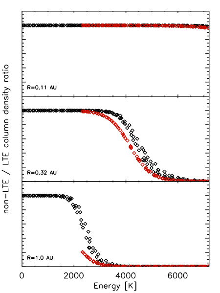
Figure 6.— The non-LTE / LTE integrated column density ratios for radii $R=0.11,0.32$, and $1.0$ AU, for levels in the ground (black) and first (red) vibrational states.

Fig. 7 shows the ratios between the non-LTE and LTE velocity integrated line fluxes in the Spitzer-IRS band. The points are marked with four different colors depending on their upper level energy. The ratios are generally less than unity, meaning that an assumption of LTE will overestimate line fluxes. The figure illustrates that: 1) the spread in the ratios is very large, 2) the lower the upper level energy $E_{up}$, the closer the ratio is to unity, 3) the overall shapes of the LTE and non-LTE line spectra (when viewed as an ensemble over the entire mid-infrared range) are very different (see also Fig. 9), and (4) the ratio shows only a shallow trend with wavelength. The last point is an indication that the upper level energies are evenly distributed with line frequency thanks to the asymmetric top nature of the water spectrum. This is particularly convenient from an observer’s perspective as it will usually be possible to observe lines with a wide range of properties even if only a limited wavelength range is available.

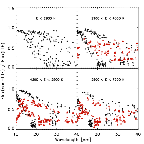
Figure 7.— Ratios of the non-LTE and LTE velocity integrated line fluxes for line with upper energy $E<2900$ K (top left), $2900<E<4300$ K (top right), $4300<E<5800$ K (bottom left), and $E>5800$ K (bottom right) in the Spitzer-IRS band. A distinction is made between the ground vibrational level (black crosses) and first vibrational level (red triangles).

Fig. 8 shows the Einstein A coefficients versus the non-LTE/LTE line flux ratios, again separated into four groups as in Fig. 7. The figure illustrates the following:

• The line flux ratios decrease for larger Einstein A coefficients. This occurs because the critical densities are higher for transitions with larger Einstein A coefficients (the de-excitation rates are comparable when the upper level energies are similar). Such transitions are therefore farthest from LTE.

• For this particular model, lines with Einstein A coefficients below $\sim 10^{-2}$ s^-1 are close to LTE.

• The ratios for transitions within the ground are higher than the first vibrational level. This is an indication that collisions dominate the excitation. If fluorescent excitation through the first vibrational bending mode were dominant then the line fluxes (at the same energy) become significantly larger for transitions from the first vibrational level that for those from the ground state.

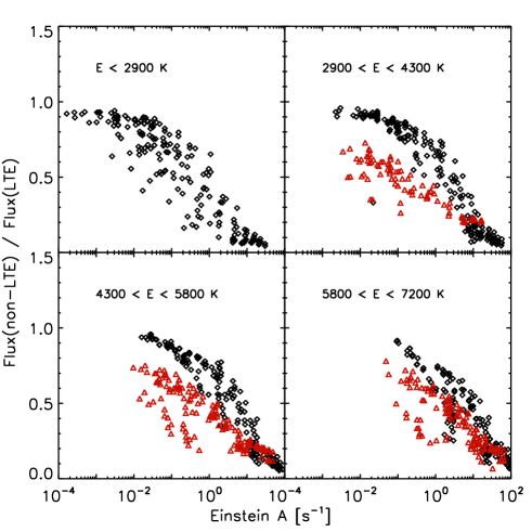
Figure 8.— Einstein A coefficients versus ratios of the non-LTE and LTE velocity integrated line fluxes for line with upper energy $E<2900$ K (top left), $2900<E<4300$ K (top right), $4300<E<5800$ K (bottom left), and $E>5800$ K (bottom right) in the Spitzer IRS band. A distinction is made between the ground vibrational level (black diamonds) and first vibrational level (red triangles).

5.2. Toward a fiducial model

Figure 9.— Comparison of non-LTE (column a) and LTE (column row) line spectra for constant abundance distribution (model 1), then adding density dependent freeze-out (model 2), decoupling gas from dust in warm atmosphere (model 3), increasing the gas to dust ratio from 1280 to 12800 (model 4), and reducing the H₂O abundance above mid-plane snowline, proposed as vertical cold finger effect (model 5), respectively.

In this section a model that qualitatively reproduces the shape of the observed H₂O line spectra is constructed. Fig. 9 shows the line spectra for five different models of non-LTE and LTE spectra convolved to two different resolutions, $\lambda/\Delta\lambda=600$ (500 km/s, Spitzer IRS) and 50000 (6 km/s). All models have the same gas density distribution (see Fig. 4), but have an increasing level of complexity of the water distribution and excitation to accommodate the observables.

Model 1 is the reference model with a gas temperature equal to the dust temperature and a constant water abundance ($x_{\rm H_{2}O}=3\times 10^{-4}$) throughout the disk, even in regions where water should freeze out. In Model 2 a density dependent freeze-out of water has been added (see Fig. 3, and Section 4.1). The main difference in the line spectra between Model 1 and 2 is that some of the low excitation lines decrease in intensity. The overall line spectrum does not change drastically in the Spitzer range with freeze-out added (especially in the non-LTE case). This is due to the relatively high excitation temperatures of the lines from $10-36$ $\mu$m as well as the fact that these transitions are subthermally excited at the location of the surface snow line. However, the freeze-out does affect lines of lower excitation, located in the spectral regime between 60 and 200$\mu$m (Meijerink et al., 2008), relevant for Herschel-PACS. Although Model 1 and 2 are able to produce bright lines of low excitation energy, similarly bright high excitation lines are also required by the observed spectra, inconsistent with these models.

One way of increasing the strength of the high excitation lines is to consider the decoupling of the gas temperature from the dust in the upper part of the atmosphere of the disk. The parametrized treatment of this decoupling, as discussed in Section 4.2, is added to Model 2, producing Model 3. Both the high and low excitation lines increase in intensity (between 20-100 percent), but the line to continuum ratios do not approach the observations, and the low excitation lines are in fact boosted more than the high excitation lines. Furthermore, the line-to-continuum ratio is still a factor of 3-5 too low with respect to representative Spitzer IRS spectra. For instance, the prominent 33 $\mu$m line complex now has a line to continuum ratio of 0.05:1 at Spitzer-IRS resolution, compared to observed values of $\sim$0.1-0.2:1.

In order to increase the general line-to-continuum ratio, Model 4 is introduced, which is the same as Model 3, except that the gas-to-dust ratio has been increased by factor of 10 to simulate strong dust settling. The result is that higher gas densities contribute near the disk surface leading to increased line intensities, coupled with a decrease in the dust continuum. This model shows a much better agreement with observations, but many low excitation lines are now too bright. Furthermore, the line spectrum shows a strong increase in peak line strength with wavelength, in contradiction with the observed, almost flat, line integrated intensities.

The reason that the low excitation lines are bright is that they are produced over a wide range of radii in the disk. Hence, they can be suppressed if the water vapor abundance is drastically lowered beyond a certain radius. Static chemical models do predict that the water abundance is lowered by 1-2 orders of magnitude at temperatures below $\sim 300~{}$K, which might be enough to reproduce some of the observed line spectra, but due to the high optical depths that remain at low temperature, the data indicate that higher depletions may be necessary. Thus, other mechanisms should be investigated. Stevenson & Lunine (1988) suggested that water vapor (and therefore oxygen) is depleted from the inner disk, within the midplane snow line, on time scales shorter than the life time of the disk. In this mechanism the water vapor is transported from just within the snow line (closer to the central star) to just outside the snow line by turbulent diffusion, at which point the water freezes out. Essentially, the sharp change in the partial pressure of water vapor across the snow line results in a net flux of water molecules outwards in the disk. However, this radial “cold finger” effect is likely balanced by the inward migration of icy bodies, as discussed in Salyk et al. (2008) and Ciesla (2009).

The radial cold finger effect assumes that the snow line is a vertical line in an isothermal disk. However, due to the temperature inversion in the disk atmosphere (Glassgold et al., 2004; Kamp & Dullemond, 2004; Woitke et al., 2009), the snow line is actually a curve that becomes almost parallel to the disk surface over a very wide range of the disk, typically the entire planet-forming region (0.5-20 AU). This can be seen in Fig. 4, and is sketched in Fig. 10. Hence, near the surface, the cold finger effect will operate in the vertical direction; water vapor will diffuse via turbulence to regions below the snow line where it will freeze out and take part in the general settling of dust to the midplane in a process one might call the “vertical cold finger” effect. The important difference relative to the radial cold finger effect is that in the surface water vapor abundance will not be replenished by the migration (in the case, the relofting) of solids if icy dust grains grow to significant size as they settle and as seems to be required by the significant millimeter-wave fluxes of many disks, particularly those that are referred to as transitional disks (see Brown, 2007). Further, the turbulence will be higher in the surface, thus shortening the water depletion time scale. Therefore, we speculate that such a mechanism is an effective means of depleting surface water above the midplane snow line. If true, this would be of considerable importance because it would mean that the radial distribution of surface water, as observed with Spitzer-IRS and future mid- to far-infrared facilities, may well trace the midplane snow line. More detailed modeling is needed to estimate whether the time scales for this proposed process are short enough to operate efficiently. It can be noted that a vertical cold finger effect truncation above the snow line at $\sim 1~{}$AU neatly explains why the slab models fit so well when assuming the same emitting area for all water lines over a wide range of excitation energies. In this way, the water emission radius derived from slab models may in fact be a measure of the location of the midplane snow line.

In Model 5 we mimic the vertical cold finger effect by setting the water abundance to the freeze-out abundance ($10^{-10}$) above the midplane snow line of the disk, as illustrated in Fig. 10. The resulting spectrum shows that the line spectrum has significantly flattened, in general agreement with the observed water spectra (see also Fig. 11).

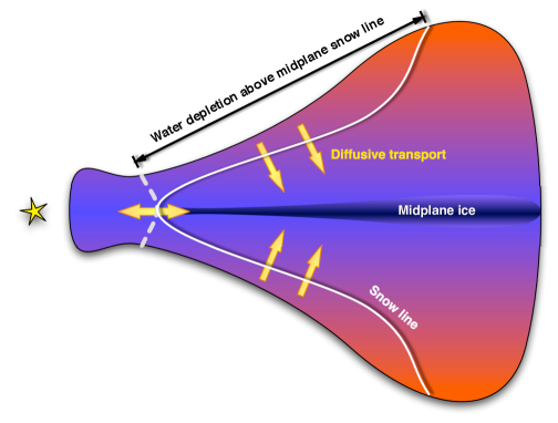
Figure 10.— Vertical cold finger effect: Water vapour will diffuse to regions below the snowline, where it will freeze out and take part in the general settling of dust to the midplane. For the fiducial model, the inner rim and the mid-plane snowline are located at R=0.07 and 0.7 AU, respectively.

6. Discussion & Conclusions

Figure 11.— Comparison of the 10-36 $\mu$m model spectra to that of AA Tau, DR Tau and AS 205A, at R=600 (Carr & Najita, 2008; Salyk et al., 2008). The spectra are normalized to the continuum.

Driven by the recent detection of hundreds of water emission lines in the mid-infrared from disks around T Tauri stars by Carr & Najita (2008) and Salyk et al. (2008), a non-LTE 2D model has been constructed that qualitatively reproduces the observed spectra. The model can be adjusted to obtain detailed fits to individual mid-infrared spectra. Our approach is to derive an abundance structure for water based on observational constraints, rather than use the prediction of existing chemistry or transport models. As a demonstration of this technique, the action of a vertical cold finger effect is proposed to model the observed truncation of the surface abundance of water vapor.

The four most important conclusions are:

1) A non-thermal excitation treatment of water is essential in determining the water distribution given an observed mid-infrared water spectrum. Assuming LTE in the calculation of H₂O line spectra is generally invalid, especially for high excitation lines. This is best illustrated in Fig. 6 and 9. The critical densities for exciting the water lines in the 10 to 36 $\mu$m region range from $n_{crit}=10^{8}-10^{12}$ cm^-2, and rapidly increase with the upper level energy. In Models 1 and 2, the difference between the LTE and non-LTE dominant line intensities is a factor of 2 to 3. In these models, the gas temperature is assumed to be equal to that of the dust, leading to faint high excitation lines. In Model 3, the surface gas temperature is increased using a parametrization based on detailed models of the gas heating (Glassgold et al., 2009). The emission of especially the low excitation lines is now boosted by a thin layer of warm H₂O in the upper part of the disk with lower densities, leading to a much larger discrepancy between the non-LTE and LTE case due to subthermal excitation. To boost the line-to-continuum ratio even more, the gas-to-dust ratio in Models 4 and 5 was increased by a factor of 10 with respect to Model 1 through 3. The low excitation lines in Model 4 now become too bright and therefore a speculative vertical cold finger effect was added in Model 5. In this case, the difference between the LTE and non-LTE spectrum is minimized because the regions of the disk that have the largest deviation from LTE contain little/no water vapor. In summary, beyond a radius $R\sim 0.3$ AU, levels having transitions in the Spitzer IRS wavelength range are sub-thermally excited, leading to biased estimates of the temperature and density distribution, emitting areas and interpretation of high resolution ($\sim 3$ km/s) line profiles when using LTE models.

2) In order to obtain more line emission from high excitation water lines ($E_{up}>3000$ K), we introduced a steep gas temperature increase at high altitudes in the disk, which is motivated by both observations and models of, e.g., the [NeII] 12.81 $\mu$m and [OI] 6300 Å lines. This increases the line strenghts by 20-100 percent, and the low excitation lines are boosted most. This is not enough, however, to reproduce the observed Spitzer IRS line-to-continuum ratios.

3) The gas-to-dust ratio must be increased by one to two orders of magnitude with respect to the canonical ISM ratio of $\sim 100-200$ in order to approach the observed line strengths and line-to-continuum ratios. An increase in gas-to-dust ratio lowers the dust opacity, allowing lines to be formed at higher densities deeper in the disk. An increase in the apparent gas-to-dust ratio can be explained by grain growth and dust settling. Increasing the gas-to-dust ratio is a more efficient way to increase line-to-continuum ratios than the decoupling of gas from dust at high altitudes in the disk because the former modification emphasizes high density gas.

4) Chemical models (e.g., Glassgold et al., 2009; Woitke et al., 2009) show that it is possible to obtain high water abundances in the transition zone from hot ($T\sim 5000$ K) to cold gas ($T\sim 100-200$ K) and that the range along the vertical axis where the maximum abundance occurs becomes smaller with radius. Below this vertical zone, closer to the midplane, water is less efficiently formed because the neutral-neutral reactions that form it (O + H₂ $\rightarrow$ OH + H followed by OH + H₂ $\rightarrow$ H₂O + H) contain activation barriers. Even so, the predicted lower limit to the water abundance ($x_{\rm H_{2}O}\sim 10^{-6}$), or a suppression by 1-2 orders of magnitude, still produces too much emission in the optically thick low excitation lines. Rather, a sharp drop in the surface water abundance by up to 4 orders of magnitude beyond $\sim 1~{}$AU better reproduces the observations. This sharp drop is difficult to explain with only static chemical models, although it is not completely ruled out that additional chemical porcesses could effectively reduce the water abundance. We speculate a vertical cold finger effect, a process in which water vapor is diffusively transported in the vertical direction to a point below the snow line where the water freezes out and takes part in the general growth and settling of solids to the midplane, may provide a viable explanation (Fig. 10). If this effect does occur and is efficient, the radial distribution of water line emission from the disk surface can become a direct tracer of the location of the midplane snow line.

A chemical suppression of the water abundance, as compared a vertical cold finger process would give rise to two completely different disk surface chemistries as a function of radius that can be tested observationally: If vertical transport is not important and chemical processes along determine the surface water abundance, the chemistry is oxygen dominated. Conversely, a vertical cold finger effect will dramatically reduce the total oxygen abundance in the surface, giving rise a carbon-dominated chemistry resulting in very different radial distributions of organics and other species as observed in mid-infrared surface molecular tracers. To test this, sensitive high resolution mid-infrared spectroscopy is required, such as will be offered by the James Webb Space Telescope (JWST) and the next generation of Extremely Large Telescopes (ELTs), combined with detailed excitation modeling.

The present study has qualitatively determined the water temperature and abundance distribution required to explain observed mid-infrared spectra of T Tauri disks. However, several important aspects that may contribute to the formation and appearance of mid-infrared water lines from protoplanetary disks are not discussed in this paper.

(i) Intrinsic line broadening: Here we adopted an intrinsic linewidth that is dominated by thermal broadening. It is possible that additional broadening from MRI driven turbulence would be able to double the intrinsic linewidth, although the small predicted values for turbulent viscosities would indicate that intrinsic line widths are indeed dominated by thermal broadening. An increase of the intrinsic line broadening would reduce the opacities in the lines, thus increasing the effective critical densities, leading to lowered intensities of the high excitation lines.

(ii) Stellar properties: The central stars in the observed Spitzer sample have masses ranging $M=0.3$ to $3.0$ M_⊙, and ages ranging from 1 to 10 Myrs, corresponding to luminosities and effective temperatures ranging from $L=0.1$ to $20$ L_⊙ and $T_{\rm eff}=2000-10000$ K, respectively. The modeling presented here has not explored dependencies on the properties of the central star.

(iii) Inner holes: The maximum dust temperature will decrease when the inner rim is located at larger radii, meaning that the high excitation lines will become less prominent in disks with inner holes, while some lower excitation lines may actually become brighter (see Pontoppidan et al. 2009).

(iv) The model setup can easily be extended to other molecular species. Work is underway to treat other observed molecular tracers in the mid-infrared, including CO, HCN, C₂H₂, OH, etc.

These aspects will be discussed in a subsequent paper dedicated to a full parameter study (Meijerink et al. 2009, in prep.).

References

- Agúndez et al. (2008) Agúndez, M., Cernicharo, J., & Goicoechea, J. R. 2008, A&A, 483, 831
- Brown (2007) Brown, J. 2007, PhD thesis, California Institute of Technology
- Carr & Najita (2008) Carr, J. S., & Najita, J. R. 2008, Science, 319, 1504
- Chiang & Goldreich (1997) Chiang, E. I., & Goldreich, P. 1997, ApJ, 490, 368
- Ciesla (2009) Ciesla, F. J. 2009, Icarus, 200, 655
- Ciesla & Cuzzi (2006) Ciesla, F. J., & Cuzzi, J. N. 2006, Icarus, 181, 178
- Dubernet & Grosjean (2002) Dubernet, M.-L., & Grosjean, A. 2002, A&A, 390, 793
- Dullemond & Dominik (2004) Dullemond, C. P., & Dominik, C. 2004, A&A, 417, 159
- Ercolano et al. (2008) Ercolano, B., Drake, J. J., Raymond, J. C., & Clarke, C. C. 2008, ApJ, 688, 398
- Faure et al. (2007) Faure, A., Crimier, N., Ceccarelli, C., Valiron, P., Wiesenfeld, L., & Dubernet, M. L. 2007, A&A, 472, 1029
- Faure et al. (2004) Faure, A., Gorfinkiel, J. D., & Tennyson, J. 2004, MNRAS, 347, 323
- Faure & Josselin (2008) Faure, A., & Josselin, E. 2008, A&A, 492, 257
- Fraser et al. (2001) Fraser, H. J., Collings, M. P., McCoustra, M. R. S., & Williams, D. A. 2001, MNRAS, 327, 1165
- Glassgold et al. (2009) Glassgold, A. E., Meijerink, R., & Najita, J. R. 2009, ApJ, 701, 142
- Glassgold et al. (1997) Glassgold, A. E., Najita, J., & Igea, J. 1997, ApJ, 480, 344
- Glassgold et al. (2004) —. 2004, ApJ, 615, 972
- Gorti & Hollenbach (2008) Gorti, U., & Hollenbach, D. 2008, ApJ, 683, 287
- Green et al. (1993) Green, S., Maluendes, S., & McLean, A. D. 1993, ApJS, 85, 181
- Grosjean et al. (2003) Grosjean, A., Dubernet, M.-L., & Ceccarelli, C. 2003, A&A, 408, 1197
- Kamp & Dullemond (2004) Kamp, I., & Dullemond, C. P. 2004, ApJ, 615, 991
- Kessler-Silacci et al. (2006) Kessler-Silacci, J., Augereau, J.-C., Dullemond, C. P., Geers, V., Lahuis, F., Evans, II, N. J., van Dishoeck, E. F., Blake, G. A., Boogert, A. C. A., Brown, J., Jørgensen, J. K., Knez, C., & Pontoppidan, K. M. 2006, ApJ, 639, 275
- Kurucz (1993) Kurucz, R. L. 1993, in Astronomical Society of the Pacific Conference Series, Vol. 44, IAU Colloq. 138: Peculiar versus Normal Phenomena in A-type and Related Stars, ed. M. M. Dworetsky, F. Castelli, & R. Faraggiana, 87–+
- Markwick et al. (2002) Markwick, A. J., Ilgner, M., Millar, T. J., & Henning, T. 2002, A&A, 385, 632
- Meijerink et al. (2008) Meijerink, R., Poelman, D. R., Spaans, M., Tielens, A. G. G. M., & Glassgold, A. E. 2008, ApJ, 689, L57
- Morrison & McCammon (1983) Morrison, R., & McCammon, D. 1983, ApJ, 270, 119
- Nomura et al. (2007) Nomura, H., Aikawa, Y., Tsujimoto, M., Nakagawa, Y., & Millar, T. J. 2007, ApJ, 661, 334
- Nomura & Millar (2005) Nomura, H., & Millar, T. J. 2005, A&A, 438, 923
- Phillips et al. (1996) Phillips, T. R., Maluendes, S., & Green, S. 1996, ApJS, 107, 467
- Poelman & Spaans (2005) Poelman, D. R., & Spaans, M. 2005, A&A, 440, 559
- Poelman & Spaans (2006) —. 2006, A&A, 453, 615
- Pontoppidan (2006) Pontoppidan, K. M. 2006, A&A, 453, L47
- Pontoppidan et al. (2009) Pontoppidan, K. M., Meijerink, R., Dullemond, C. P., & Blake, G. A. 2009, ArXiv:0908.2997
- Raymond et al. (2004) Raymond, S. N., Quinn, T., & Lunine, J. I. 2004, Icarus, 168, 1
- Rothman et al. (2005) Rothman, L. S., Jacquemart, D., Barbe, A., Chris Benner, D., Birk, M., Brown, L. R., Carleer, M. R., Chackerian, C., Chance, K., Coudert, L. H., Dana, V., Devi, V. M., Flaud, J.-M., Gamache, R. R., Goldman, A., Hartmann, J.-M., Jucks, K. W., Maki, A. G., Mandin, J.-Y., Massie, S. T., Orphal, J., Perrin, A., Rinsland, C. P., Smith, M. A. H., Tennyson, J., Tolchenov, R. N., Toth, R. A., Vander Auwera, J., Varanasi, P., & Wagner, G. 2005, Journal of Quantitative Spectroscopy and Radiative Transfer, 96, 139
- Salyk et al. (2008) Salyk, C., Pontoppidan, K. M., Blake, G. A., Lahuis, F., van Dishoeck, E. F., & Evans, II, N. J. 2008, ApJ, 676, L49
- Siess et al. (2000) Siess, L., Dufour, E., & Forestini, M. 2000, A&A, 358, 593
- Stevenson & Lunine (1988) Stevenson, D. J., & Lunine, J. I. 1988, Icarus, 75, 146
- Woitke et al. (2009) Woitke, P., Kamp, I., & Thi, W.-F. 2009, A&A, 501, 383
- Woods & Willacy (2009) Woods, P. M., & Willacy, K. 2009, ApJ, 693, 1360