Gravitational-wave memory and pulsar timing arrays.

Abstract

Pulsar timing arrays (PTAs) are designed to detect gravitational waves with periods from several months to several years, e.g. those produced by by wide supermassive black-hole binaries in the centers of distant galaxies. Here we show that PTAs are also sensitive to mergers of supermassive black holes. While these mergers occur on a timescale too short to be resolvable by a PTA, they generate a change of metric due to non-linear gravitational-wave memory which persists for the duration of the experiment and could be detected. We develop the theory of the single-source detection by PTAs, and derive the sensitivity of PTAs to the gravitational-wave memory jumps. We show that mergers of $10^{8}M_{\odot}$ black holes are $2-\sigma$-detectable (in a direction, polarization, and time-dependent way) out to co-moving distances of $\sim 1$ billion light years. Modern prediction for black-hole merger rates imply marginal to modest chance of an individual jump detection by currently developed PTAs. The sensitivity is expected to be somewhat higher for futuristic PTA experiments with SKA.

1 introduction

Bursts of gravitational waves leave a permanent imprint on spacetime by causing a small permanent change of the metric, as computed in the transverse traceless gauge (Payne 1983; Christodoulou 1991; Blanchet & Damour 1992; Thorne 1992). This gravitational-wave “memory jumps” are particularly significant in the case of merger of a binary black hole, as was recently pointed out by Favata (2009, hereafter F09). Favata has shown (see Figure 1 of F09) that for the case of an equal-mass binary, a metric memory jump $\delta h$ was of the order of $\sim 5$ percent of $M/R$, where $M$ is the mass of the binary component and $R$ is the co-moving distance to the binary measured at redshift $0$ (hereafter $M$ is expressed in the geometric units, i.e. $M=GM/c^{2}$). Furthermore, Favata has argued that the memory jumps were potentially detectable by LISA with high signal-to-noise ratio. Favata’s memory calculations make use of an approximate analytical treatment of the mergers, and need to be followed up with more definitive numerical calculations. Nevertheless, a number of analytical models explored in F09 show that the effect is clearly of high importance, and thus further investigations of detectability of the memory jumps are warranted.

Recently, there has been a renewed effort to measure gravitational waves from widely separated supermassive black-hole (SMBH) binaries by using precise timing of galactic millisecond pulsars (Jenet et al. 2005; Manchester 2006). In this paper we investigate whether pulsar timing arrays (PTAs) could be sensitive to the memory jumps from physical mergers of the SMBHs at the end of the binary’s life. We demonstrate that modern PTAs (Manchester 2006), after $~{}10$ years of operation, will be sensitive to mergers of $10^{8}M_{\odot}$ black holes out to $\sim$billion light years; however the chances of actual detection are small. Futuristic PTA experiments, like those performed on the Square Kilometer Array (Cordes et al. 2005), offer a somewhat better prospect for the direct detection of gravitational-wave memory jumps.

2 the signal

The gravitational waveform from a merger of SMBH pair consists of an ac-part and a dc-part; see Figure 1 of F09. The ac-part is short-period and short-lived, and hence is undetectable by a PTA. The dc-part is the gravitational-wave memory; it grows rapidly during the merger, on the timescale of $\sim 10M(1+z)\simeq 10^{4}(M/10^{8}M_{\odot})(1+z)\hbox{s}$, where $M$ is the mass of the SMBHs (assumed equal) and $z$ is the redshift of the merger. After the burst passes, the change in metric persists, and as we explain below, it is this durable change in the metric that makes the main impact on the timing residuals. Realistic PTA programs are designed to clock each of the pulsars with $\sim 2$-week intervals (Manchester 2006, Bailes, private communications). Therefore, for $M=10^{8}M_{\odot}$ SMBHs the growth of the memory-related metric change is not time-resolved by the timing measurements. Moreover, even for $M=10^{10}M_{\odot}$ SMBHs this growth occurs on the timescale much shorter than the duration on the experiment. We are therefore warranted to treat the dc-part of the gravitational wave as a discontinuous jump propagating through space,

$$h(\vec{r},t)=h_{0}\times\Theta\left[(t-t_{0})-\vec{n}\cdot\vec{r}\right],$$ (1)

where $h_{0}$ is the amplitude of the jump, of the order of $0.05M/R$, $\Theta(t)$ is the Heavyside function, $t_{0}$ is the moment of time when the gravitational-wave burst passes an observer, $\vec{r}$ is the location in space relative to the observer, and $\vec{n}$ is the unit vector pointed in the direction of the wave propagation. Here and below we set $c=1$. We have used the plane-wave approximation, which is justified for treating extragalactic gravitational waves as they propagate through the Galaxy.

For a single pulsar, the frequency of the pulse-arrival $\nu$ responds to a plane gravitational wave according to the following equation (Estabrook & Wahlquist 1975; Hellings & Downs 1983):

$${\delta\nu(t)\over\nu} = B(\theta,\phi)\times\left[h(t)-h(t-r-r\cos\theta)\right],$$ (2)

where

$$B(\theta,\phi)={1\over 2}\cos(2\phi)\left(1-\cos\theta\right).$$ (3)

Here $r$ is the Earth-pulsar distance at an angle $\theta$ to the direction of the wave propagation, $\phi$ is the angle between the wave’s principle polarization and the projection of the pulsar onto the plane perpendicular to the propagation direction, and $h(t)$ is the gravitational-wave strain at the observer’s location. Substituting Eq. (1) into the above equation, we obtain the mathematical form of the signal:

$${\delta\nu(t)\over\nu}=h_{0}B(\theta,\phi)\times\left[\Theta(t-t_{0})-\Theta(t-t_{1})\right],$$ (4)

where $t_{1}=t_{0}+r(1+\cos\theta)$. Thus the memory jump would cause a pair of pulse frequency jumps of equal magnitude and the opposite sign, separated by the time interval $r(1+\cos\theta)$. Since typical PTA pulsars are at least $\sim 10^{3}$ light years away, a single merger could generate at most one of the frequency jumps as seen during the $\sim 10$ years of a PTA experiment. The timing residuals from a single jump at $t=t_{0}$ are given by

$$m(t)=B(\theta,\phi)h_{0}\times\Theta(t-t_{0})\times(t-t_{0}).$$ (5)

For a single pulsar the frequency jump is indistinguishable from a fast glitch, and therefore single-pulsar data can only be used for placing upper limits on gravitational-wave memory jumps. The situation would be different for an array of pulsars, where simultaneous pulse frequency jumps would occur in all of them at the time $t=t_{0}$ when the gravitational-wave burst would reach the Earth. Therefore a PTA could in principle be used to to detect memory jumps.

3 Single-source detection by PTAs.

In this section we develop a mathematical framework for the single-source detection by a PTA. Our formalism is essentially Bayesian and follows closely the spirit of van Haasteren et al. (2009, hereafter vHLML), although we will make a connection with the frequentist Wiener-filter estimator. We will then apply our general formalism to the memory jumps. The reader uninterested in mathematical details should skip the following subsection and go straight to the results in section 5.

There is a large body of literature on the single-source detection in the gravitational-wave community (Finn 1992; Owen 1996; Brady et al. 1998). The techniques which have been developed so far are designed specifically for the interferometric gravitational-wave detectors like LIGO and LISA. There are several important modifications which need to be considered when applying these techniques to PTAs, among them
1. Discreteness of the data set. A single timing residual per observed pulsar is obtained during the observing run; these runs are separated by at least several weeks. This is in contrast to the continuous (for all practical purposes) data stream in LIGO and LISA.
2. Subtraction of the systematic corrections. The most essential of these is the quadratic component of the timing residuals due to pulsar spindown, but there may be others, e.g. jumps of the zero point due to equipment change, annual modulations, etc.
3. Duration of the signal may be comparable to the duration of the experiment. This is the case for both cosmological stochastic background considered in vHLML, and for the memory jumps considered here. Thus frequency domain methods are not optimal, and time-domain formalism should be developed instead.

The Bayesian time-domain approach developed in vHLML and in this subsection is designed to tackle these 3 complications.

Consider a collection of $N$ timing residuals $\delta t_{p}$ obtained from clocking a number of pulsars. Here $p$ is the composite index meant to indicate both the pulsar and the observing run together. Mathematically, we represent the residuals as follows:

$$\delta t_{p}=A\times s(t_{p})+\delta t^{n}_{p}+Q(t_{p}).$$ (6)

Here $s(t_{p})$ and $A$ are the known functional form and unknown amplitude of a gravitational-wave signal from a single source, $\delta t^{n}_{p}$ is the stochastic contribution from a combination of the timing and receiver noises, and

$$Q(t_{p})=\Sigma_{m}\xi_{m}f_{m}(t_{p})$$ (7)

is the contribution from systematic errors of known functional forms $f_{m}(t_{p})$ but a-priory unknown magnitudes $\xi_{m}$. Below we shall specify $Q(t_{p})$ to be the unsubtracted part of the quadratic spindown, however for now we prefer to keep the discussion as general as possible. We follow van Haasteren et al. (2009) and rewrite Eq. (6) in a vector form:

$$\vec{\delta t}=A\vec{s}+\vec{\delta t}^{n}+F\vec{\xi}.$$ (8)

Here the components of the column vectors $\vec{\delta t}$, $\vec{\delta t}^{n}$, $\vec{s}$, and $\vec{\xi}$ are given by $\delta t_{p}$, $\delta t^{n}_{p}$, $s(t_{p})$, and $\xi_{m}$, and $F$ is a non-square matrix with the elements $F_{pm}=f_{m}(t_{p})$. Henceforth we assume that $\delta t^{n}_{p}$ is the random Gaussian process, with the symmetric positive-definite coherence matrix $C$:

$$C_{pq}=<\delta t^{n}_{p}\delta t^{n}_{q}>.$$ (9)

We can now write down the joint probability distribution for $A$ and $\xi_{m}$:

$$P(A,\xi_{m}|\vec{\delta t}) = {(1/M)}P_{0}(A,\xi_{m})\times$$

$$\exp\left[-{1\over 2}(\vec{\delta t}-A\vec{s}-F\vec{\xi})^{T}\times C^{-1}\times,\right.$$

$$\left.(\vec{\delta t}-A\vec{s}-F\vec{\xi})\right].$$

Here $P_{0}(A,\xi_{m})$ is the prior probability distribution, and $M$ is the overall normalization factor. We now assume a flat prior $P_{0}(A,L_{m})=const$, and marginalize over $\vec{\xi}$ in precisely the same way as shown in the Appendix of vHLML. As a result, we get the following Gaussian probability distribution for $A$:

$$P(A|\vec{\delta t})={1\over\sqrt{2\pi}\sigma}\exp\left[-{(A-\bar{A})^{2}\over 2\sigma^{2}}\right].$$ (11)

Here, the mean value $\bar{A}$ and the standard deviation $\sigma$ are given by

$$\bar{A}={\vec{s}^{T}C^{\prime}\vec{\delta t}\over\vec{s}^{T}C^{\prime}\vec{s}},$$ (12)

and

$$\sigma=\left(\vec{s}^{T}C^{\prime}\vec{s}\right)^{-1/2},$$ (13)

where

$$C^{\prime}=C^{-1}-C^{-1}F\left(F^{T}C^{-1}F\right)^{-1}F^{T}C^{-1}.$$ (14)

It is instructive and useful to re-write the above equations by introducing an inner product $\langle\vec{x},\vec{y}\rangle$ defined as

$$\langle\vec{x},\vec{y}\rangle=\vec{x}^{T}C^{-1}\vec{y}.$$ (15)

Let us choose an orthonormal basis $\hat{f}_{i}$ in the subspace spanned by $\vec{f}_{m}$, so that $\langle\hat{f}_{i},\hat{f}_{j}\rangle=\delta_{ij}$. We also introduce a projection operator

$$R=1-\Sigma_{m}\left|\hat{f}_{m}\rangle\langle\hat{f}_{m}\right|,$$ (16)

so that $R\vec{x}=\vec{x}-\Sigma_{m}\langle\hat{f}_{m},\vec{x}\rangle\hat{f}_{m}$. All the usual identities for projection operators are satisfied, i.e. $R^{2}=R$ and $\langle R\vec{x},R\vec{y}\rangle=\langle\vec{x},R\vec{y}\rangle$. We can then write

$$\bar{A}={\langle\vec{s},R\vec{\delta t}\rangle\over\langle\vec{s},R\vec{s}\rangle},$$ (17)

and

$$\sigma=\langle\vec{s},R\vec{s}\rangle^{-1/2}.$$ (18)

If there are no systematic errors that need to be removed, than $R=1$ and the Eqs (17) and (18) represent the time-domain version of the Wiener-filter estimator.

3.1 Other parameters

So far we have assumed that the gravitational-wave signal has a known functional form but unknown amplitude, and have explained how to measure or constrain this amplitude. In reality, the waveform $\vec{s}(\vec{\eta},t_{P})$ will depend on a number of a-priori unknown parameters $\vec{\eta}$, such as the starting time of the gravitational-wave burst and the direction from which this burst has come. These parameters enter into the probability distribution function through $\vec{s}$ in Eq. (3), and generally their distribution functions have to be estimated numerically. The estimates can be done via the matched filtering (Owen 1996) or by performing Markov-Chain Monte-Carlo (MCMC) simulations. In section 5, we will demonstrate an example of an MCMC simulation for the memory jump. In this section, we show how to estimate an average statistical error on $\vec{\eta}$ for signals with high signal-to-noise ratios.

Let us begin with a joint likelihood function for the amplitude $A$ and other parameters $\eta$:

$$L(A,\vec{\eta})=-(1/2)\langle A\vec{s}(\vec{\eta})-\vec{\delta t},R(A\vec{s}(\vec{\eta})-\vec{\delta t})\rangle+Const.$$ (19)

We now fix $A$ to its maximum-likelihood value $\langle\vec{s}(\vec{\eta}),R\vec{\delta t}\rangle/\langle\vec{s}(\vec{\eta}),R\vec{s}(\vec{\eta})\rangle$, and average over a large number of statistical realizations of the noise $\vec{\delta t}^{n}$. The so-averaged likelihood function is given by

$$L_{\rm av}(\vec{\eta}) = -{(1/2)A_{t}^{2}\over\langle\vec{s}(\vec{\eta}),R\vec{s}(\vec{\eta})\rangle}\left[\langle\vec{s}(\vec{\eta}_{t}),R\vec{s}(\vec{\eta}_{t})\rangle\langle\vec{s}(\vec{\eta}),R\vec{s}(\vec{\eta})\rangle-\right.$$ (20)

$$\left.\langle\vec{s}(\vec{\eta}_{t}),R\vec{s}(\vec{\eta})\rangle^{2}\right],$$

where $A_{t},\vec{\eta}_{t}$ are the true values for the signal present in all data realizations. We have omitted the additive constant.

The expression in the square bracket is positive-definite, and $L_{\rm av}$ is quadratic in $\vec{\eta}-\vec{\eta}_{t}$ for the values of $\vec{\eta}$ close to the true values,

$$L_{\rm av}(\vec{\eta})\simeq-(1/2)(\vec{\eta}-\vec{\eta}_{t})G(\vec{\eta}-\vec{\eta}_{t}),$$ (21)

where $G$ is the positive-definite Fisher information matrix. Its elements can be expressed as

$$G_{ij} = {A_{t}^{2}/\langle\vec{s},R\vec{s}\rangle}\left[\langle\vec{s},R\vec{s}\rangle\langle{\partial\vec{s}\over\partial\eta_{i}},R{\partial\vec{s}\over\partial\eta_{j}}\rangle-\right.$$ (22)

$$\left.\langle\vec{s},R{\partial\vec{s}\over\partial\eta_{i}}\rangle\langle\vec{s},R{\partial\vec{s}\over\partial\eta_{j}}\rangle\right],$$

evaluated at $\eta=\eta_{t}$. The inverse of $G$ specifies the average error with which parameters $\vec{\eta}$ can be estimated from the data.

4 detectability of memory jumps

We now make an analytical estimate for detectability of the memory jumps. For simplicity, we assume that all of the pulsar observations are performed regularly so that the timing-residual measurements are separated by a fixed time $\Delta t$, and that the whole experiment lasts over the time interval $[-T,T]$ (expressed in this way for mathematical convenience). Furthermore, we assume that the timing/receiver noise is white, i.e. that for a pulsar $a$

$$\langle\delta t^{n}_{i}\delta t^{n}_{j}\rangle=\sigma_{a}^{2}\delta_{ij}.$$ (23)

This assumption is probably not valid for some of the millisecond pulsars (Verbiest et al., in prep., van Haasteren et al., in prep.). We postpone discussion of the non-white noises to future work.

To keep our exposition transparent, we consider the case when the array consists of a single pulsar $a$; generalization to several pulsars is straightforward and is shown later this section. Finally, we assume that the systematic error $Q(t_{i})$ comprises only an unsubtracted component of the quadratic spindown,

$$Q(t_{i})=A_{0}+A_{1}t_{i}+A_{2}t_{i}^{2},$$ (24)

where $A_{0}$, $A_{1}$, and $A_{2}$ are a-priori unknown parameters.

We now come back to the formalism developed in the previous section. The inner product defined in Eq. (15) takes a simple form:

$$\langle\vec{x},\vec{y}\rangle = {1\over\sigma_{a}^{2}}\sum_{i}x(t_{i})y(t_{i})$$

$$\simeq {1\over\sigma_{a}^{2}\Delta t}\int_{-T}^{T}x(t)y(t)dt,$$

where we have assumed $\Delta t\ll T$ and have substituted the sum with the integral in the last equation. We now choose orthonormal basis vectors $\hat{f}_{1,2,3}(t)$ which span the linear space of quadratic functions:

$$\hat{f}_{1}(t) = \sigma_{a}\sqrt{\Delta t\over T}{1\over\sqrt{2}}$$ (26)

$$\hat{f}_{2}(t) = \sigma_{a}\sqrt{\Delta t\over T}\sqrt{3\over 2}{t\over T}$$

$$\hat{f}_{3}(t) = \sigma_{a}\sqrt{\Delta t\over T}\sqrt{45\over 8}\left[\left({t\over T}\right)^{2}-{1\over 3}\right].$$

From Eq. (5) the gravitational-wave induced timing residuals are given by $\delta t(t)=h_{0}s(t)$, where

$$s(t)=B(\theta,\phi)\times\Theta(t-t_{0})\times(t-t_{0}).$$ (27)

The expected measurement error of the jump amplitude $h_{0}$ is given by Eq. (18):

$$\sigma_{h_{0}}=\left[\langle\vec{s},\vec{s}\rangle^{2}-\sum_{i=1,2,3}\langle\vec{s},\hat{f}_{i}\rangle^{2}\right]^{-1/2}.$$ (28)

Substituting Eqs. (4), (26), and (27) into Eq. (28), one gets after some algebra:

$$\sigma_{h_{0}}={1\over B(\theta,\phi)}{\sigma_{a}\over T}\sqrt{48\over Np^{3}\left(1-{15\over 16}p\right)}.$$ (29)

Here $N=2T/\Delta t$ is the number of measurements, and

$$p=1-\left(t_{0}/T\right)^{2}.$$ (30)

For an array consisting of multiple pulsars, and with the assumption that the timing residuals are obtained for all of them during each of the $N$ observing runs, the above expression for $\sigma_{h_{0}}$ is modified as follows:

$$\sigma_{h_{0}}={\sigma_{\rm eff}\over T}\sqrt{48\over Np^{3}\left(1-{15\over 16}p\right)},$$ (31)

where

$$\sigma_{\rm eff}=\left[\sum_{a}\left(B^{2}(\theta_{a},\phi_{a})/\sigma_{a}^{2}\right)\right]^{-1/2}.$$ (32)

Several remarks are in order:

1. The error $\sigma_{h_{0}}$ diverges when $p=0$, i.e. when $t_{0}=\pm T$. This is as expected: when the memory jump arrives at the beginning or at the end of the timing-array experiment, it gets entirely fitted out when the pulsar spin frequency is determined, and is thus undetectable.

2. Naively, one may expect the optimal sensitivity when the jump arrives exactly in the middle of the experiment’s time interval, i.e. when $t_{0}=0$. This is not so; the optimal sensitivity is achieved for $t_{0}/T=\pm 1/\sqrt{5}$ when the error equals

$$\sigma_{h_{0}}={\sigma_{\rm eff}\over T}\sqrt{375\over N}.$$ (33)

3. The sky-average value for $B^{2}(\theta,\phi)$ is $1/6$. Therefore, for an array consisting of a large number of pulsars $N_{p}$ which are distributed in the sky isotropically and which have the same amplitude of timing/receiver noise $\sigma_{a}=\sigma$, the $\sigma_{\rm eff}$ in Eq. (31) is given by

$$\sigma_{\rm eff}=\sigma\sqrt{6/N_{p}}.$$ (34)

4. While the timing precision of future timing arrays is somewhat uncertain, it is instructive to consider a numerical example. Lets assume $T=5$yr (i.e., the 10-year duration of the experiment), $N=250$ (i.e., roughly bi-weekly timing-residual measurements), $N_{p}=20$ isotropically-distributed pulsars (this is the current number of clocked millisecond pulsars), and $\sigma_{a}=100$ns (this sensitivity is currently achieved for only several pulsars). Then for optimal arrival time $t_{0}=\pm T/\sqrt{5}$, the array sensitivity is

$$\sigma_{h_{0}}=4.5\times 10^{-16}.$$ (35)

For a binary consisting of two black holes of the mass $M$, the memory jump is estimated in F09 to be

$$h_{0}=\eta{M\over R}\simeq 8\times 10^{-16}{\eta\over 0.05}\left({M\over 10^{8}M_{\odot}}\right)\left({10^{9}\hbox{light-years}\over R}\right),$$ (36)

where $\eta\sim 0.05$ is the direction-dependent numerical parameter. In this example, the pulsar-timing array is sensitive to the memory jumps from black-hole mergers at redshifts $z<z_{0}$, where $z_{0}\sim 0.1$ for $M=10^{8}M_{\odot}$, and $z_{0}\sim 1$ for $M=10^{9}M_{\odot}$.

4.1 Arrival time

It is possible to estimate the array’s sensitivity to the memory-jump arrival time, $t_{0}$. We use Eqs. (22) and (27), and after some algebra get

$$\sigma_{t_{0}}=T\left({h_{0}T\over\sigma_{\rm eff}}\right)^{-1}\sqrt{2/N}\chi(p),$$ (38)

where

$${1\over\chi^{2}(p)}={1\over 2}p\left(1+{5\over 4}p^{2}-2p\right)-{3(1-p)p\left[1-(5/8)p\right]^{2}\over 2[1-(15/16)p]}.$$ (39)

4.2 Source position

The array’s sensitivity gravitational-wave memory is dependent on source position since the number and the position of the pulsars in current PTAs is not sufficient to justify the assumption of isotropy made in Eq. (34). We will therefore calculate the value of $\left[\sum_{a}B^{2}\left(\theta_{a},\phi_{a}\right)\right]^{-1/2}$ for current PTAs. Since the polarisation of the gravitational-wave memory signal is an unknown independent parameter, we average over the polarisation and obtain for the angular sensitivity:

$$\sigma_{h_{0}}\left(\phi_{s},\theta_{s}\right) \sim \left[\sum_{a}B^{2}\left(\phi_{s},\theta_{s},\theta_{a},\phi_{a}\right)\right]^{-1/2}$$ (40)

$$= \left[\sum_{a}\frac{1}{8}\left(1+\cos\theta_{a}\left(\phi_{s},\theta_{s}\right)\right)^{2}\right]^{-1/2}.$$ (41)

Here we have assumed that all pulsars have equal timing precision. $\phi_{s}$ and $\theta_{s}$ are the position angles of the gravitational-wave memory source, and $\theta_{a}$ is the polar angle of pulsar $a$ in a coordinate system with $\left(\phi_{s},\theta_{s}\right)$ at the north-pole. In figure 1 and 2 the sensitivity to different gravitational-wave memory source positions is shown for respectively the European Pulsar Timing Array and the Parkes Pulsar Timing Array projects.

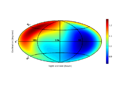
Figure 1: The relative sensitivity $\sigma_{\rm eff}$ for the pulsars of the European Pulsar Timing Array. The scaling has been chosen such that a value of $1$ indicates that the same sensitivity for that source position would have been achieved with a perfect isotropic PTA (i.e. $B^{2}=\frac{1}{6}$)

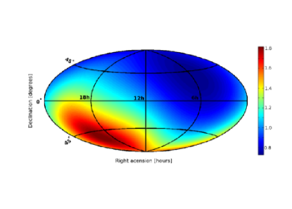
Figure 2: The relative sensitivity $\sigma_{\rm eff}$ for the pulsars of the Parkes Pulsar Timing Array. The scaling has been chosen such that a value of $1$ indicates that the same sensitivity for that source position would have been achieved with a perfect isotropic PTA (i.e. $B^{2}=\frac{1}{6}$)

5 Tests using mock data

We test the array’s sensitivity to gravitational-wave memory signals using mock timing residuals for a number of millisecond pulsars. In this whole section, all the mock timing residuals were generated in two steps:
1) A set of timing residuals was generated using the pulsar timing package tempo2 (Hobbs et al. 2006). We assume that the observations are taken tri-weekly over a time-span of $10$ years. The pulsar timing noise was set to $100$ ns white noise.
2) A gravitational-wave memory signal was added according to Eq. (5), with a memory-jump arrival time set to be optimal for sensitivity: $\frac{t_{0}}{T}=\frac{1}{\sqrt{5}}$. The direction and polarisation of the gravitational-wave memory signal were chosen randomly - the coordinates happened to have declination $90^{o}$.
In the following subsections we describe tests which have fixed parameters for step 1, but systematically varied amplitude for step 2, and we use these tests to study the sensitivity of the array.

5.1 Used models

In principle, we would like to realistically extrapolate the results we obtain here for mock datasets to future real datasets from PTA projects. Several practical notes are in order to justify the models we use here to analyse the mock datasets:
1) From equation (24) onward, we assume that the systematic-error contributions to the timing residuals consist only of the quadratic spindown. In reality, pulsar observers must fit many model parameters to the data, and have developed appropriate fitting routines within timing packages like tempo2. Similar to the quadratic spindown discussed in this paper, all the parameters of the timing model are linear or linearised in tempo2, and therefore those parameters are of known functional form. Since the subtraction of quadratic spindown decreases the sensitivity of the PTA to gravitational-wave memory signals, we would expect the same thing to be true for the rest of the timing model.
2) The error-bars on the pulse arrival time obtained from correlating the measured pulse-profile with the template of the pulse-profile are generally not completely trusted. Many pulsar astronomers invoke an extra “fudge” factor that adjusts the error-bars on the timing-residuals to make sure that the errors one gets on the parameters of the timing-model are not underestimated. Usually the “fudge” factor, which is known as an $efac$ value is set to the value which makes the reduced $\chi^{2}$ of the timing solution to be equal to $1$.

In order to check the significance of both limitations 1 & 2, we perform the following test. We take a realistic set of pulsars with realistic timing models: the pulsar positions and timing models of the PPTA pulsars. We then simulate white timing-residuals and a gravitational-wave memory signal with amplitude $h_{0}=10^{-15}$, and we produce the posterior distribution of Eq. (11) in three different ways:
a) We marginalise over only the quadratic functions of Eq. (26), which should yield the result of Eq. (31).
b) We marginalise over the all timing model parameters included in the tempo2 analysis when producing the timing-residuals.
c) We marginalise over all the timing model parameters, and we also marginalise over the efac values using the numerical techniques of vHLML. By estimating the efac value simultaneously with the gravitational-wave memory signal, we are able to completely separate the two effects. Note that this procedure will not destroy information about the relative size of the error-bars for timing-residuals of the same pulsar.

We present the result of this analysis in Figure 3. Based on the $185$ observations per pulsar in the dataset and the direction of the gravitational-wave memory signal, we can calculate the theoretical sensitivity of the array using Eq. (33) and Eq. (34). This yields a value of:

$$\sigma_{h_{0}}=6.4\times 10^{-16}.$$ (42)

We can also calculate this value for the three graphs in Figure 3. The three graphs lie close enough on top of each other to conclude that one value applies to all three of them:

$$\sigma_{h_{0}}=6.5\times 10^{-16},$$ (43)

which is in good agreement with the theoretical value. It appears that both note 1 and 2 mentioned above are not of great influence to the sensitivity of PTAs to gravitational-wave memory detection; the theoretical calculations of this paper are a good representation of the models mentioned in this section.

Figure 3: The posterior distribution of the gravitational-wave memory amplitude. The two solid lines are the result of an analysis where we only analytically marginalise over the full timing model or just quadratic spindown. The points are the result of a marginalisation over the full timing model and the efac values as well. From the Gaussians, the sensitivity can be reliably estimated at: $\sigma_{h_{0}}=\frac{FWHM}{2\sqrt{2\ln 2}}=6.5\times 10^{-16}$

5.2 Upper-limits and detecting the signal

When there is no detectable gravitational-wave memory signal present in the data, we can set some upper-limit on the signal amplitude using the algorithm presented in this paper. Here we will analyse datasets with no or no fully detectable gravitational-wave memory signal in it, and a dataset with a well-detectable signal using the MCMC method of vHLML. We will calculate the marginalised posterior distributions for the $5$ parameters of the gravitational-wave memory signal. The interesting parameters in the case of an upper-limit are the amplitude and the arrival time of the jump. A marginalised posterior for those two parameters are then presented as two-dimensional posterior plots. Note that the difference with the analysis in section 5.1 is that we vary all gravitational-wave memory parameters, instead of only the amplitude. Note that we do marginalise over all the efac values as discussed in section 5.1, unless stated otherwise.

In Figure 4 we show the result of an analysis of a dataset where we have not added any gravitational-wave memory signal to the timing-residuals. The $3-\sigma$ contour is drawn, which serves as an upper-limit to the memory amplitude. We see that we can exclude a gravitational-wave memory signal at $\frac{t_{0}}{T}=\frac{1}{\sqrt{5}}$ of amplitude $3\times 10^{-15}$ and higher. We see that this value is over a factor of $4$ higher than what is predicted by Eq. (42). This is to be expected, since:
1) We give a $3-\sigma$ limit here, instead of the $1-\sigma$ sensitivity.
2) We also marginalise over the arrival time and other parameters of the memory signal, reducing the sensitivity.
Because of these reasons, we argue that the minimal upper-limit one can set on the gravitational-wave memory signal using a specific PTA is the sensitivity calculated using Eq. (42) multiplied by $4$.

Next we produce a set of timing-residuals with a memory signal of amplitude $h_{0}=10^{-15}$. According the result mentioned above, the memory signal should not be resolvable with this timing precision. The result is shown in Figure 5. We see that we can indeed merely set an upper-limit again. In order to check the effect of marginalising over the efac values as mentioned in section 5.1, we also perform an analysis where we pretend we do know the efac values prior to the analysis. The result is shown in Figure 6. We see no significant difference between the two models.

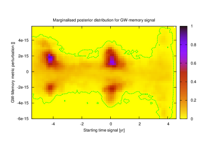
Figure 4: The marginalised posterior distribution for the gravitational-wave memory signal amplitude and arrival time of the jump. In this case a dataset was analysed that did not contain any gravitational-wave memory signal.

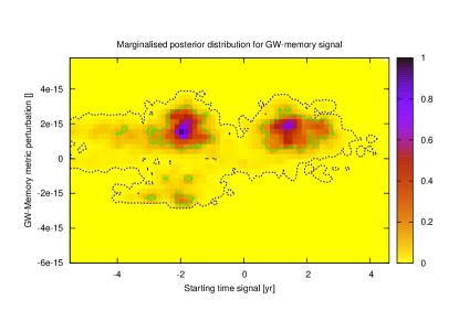
Figure 5: The marginalised posterior distribution for the gravitational-wave memory signal amplitude and arrival time of the jump. Here a gravitational-wave signal with an amplitude of $10^{-15}$ was added to the white residuals. The contour drawn is the $3-\sigma$ contour.

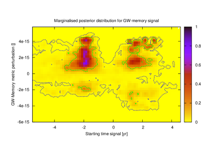
Figure 6: The marginalised posterior distribution for the gravitational-wave memory signal amplitude and arrival time of the jump. Here a gravitational-wave signal with an amplitude of $10^{-15}$ was added to the white residuals. This analysis has been done without marginalising over the efac values. The contour drawn is the $3-\sigma$ contour.

Finally, we also analyse a dataset with a gravitational-wave memory signal with an amplitude larger than the $3\times 10^{-15}$ upper-limit of the white set mentioned above. Here we have added a memory signal with an amplitude of $10^{-14}$. In Figure 7 we see that we have a definite detection of the signal: if we consider the $3-\sigma$ contours, we see that we can restrict the gravitational-wave memory amplitude between $\left[6.6\times 10^{-15},1.35\times 10^{-14}\right]$. Again, this value is higher than the value predicted by Eq. (42) due to us including more parameters in the model than just the memory amplitude. In Figure 8 we see that we can also reliably resolve the position of the source in this case.

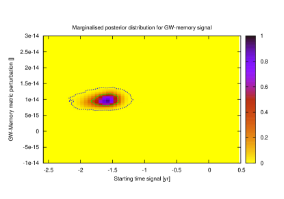
Figure 7: The marginalised posterior distribution for the gravitational-wave memory signal amplitude and arrival time of the jump. Here a gravitational-wave signal with an amplitude of $10^{-14}$ was added to the white residuals, indicated with a ’+’ in the figure. The contours drawn are the $1-\sigma$ and $3-\sigma$ contours.

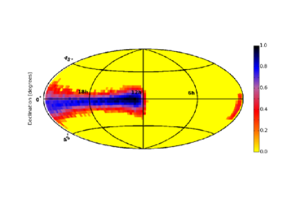
Figure 8: The marginalised posterior distribution for the sky location of the gravitational-wave memory signal. We can see here that we can marginally determine the direction of the source. The source positions used to generate the residuals were: (declination, right ascension) = ($90^{0},12.4\hbox{hr}$).

6 Discussion

In this paper, we have shown that gravitational-wave memory signals from SMBH binary mergers are in principle detectable by PTAs, and that $2-\sigma$ constraints are possible on $M=10^{8}M_{\odot}$ mergers out to redshift of $\sim 0.1$ (while those with $M=10^{10}M_{\odot}$ should be detectable throughout the Universe). How frequently do these mergers occur during the PTA lifetime? Recent calculations of Sesana et al. (2007, SVH) are not too encouraging. SVH compute, for several models of SMBH merger trees, the rate of SMBH mergers as seen on Earth, as a function of mass (their figure 1d), as well as a multidute of other parameters for these mergers. From their plots one infers few$\times 10^{-2}-10^{-3}$ PTA-observable mergers per year, which converts to at most $0.1-0.01$ detected mergers during the PTA lifetime of $\sim 10$ years (NB: during the PTA existence, only a fraction of time will spent near the arrival times with optimal sensitivity). It is conceivable that SVH estimates are on the conservative side, since the mergers of heavy black holes may be stalled (due to the “last parsec” problem) and may occur at a significantly later time than the mergers of their host halos. In this case, some fraction of high-redshift mergers may be pushed towards lower redshifts and become PTA-detectable. Detailed calculations are needed to find out whether this process could substantially increase the rate of PTA-detectable mergers. It is also worth pointing out that a futuristic PTA experiment based on a Square Kilometer Array may attain up to an order of magnitude higher sensitivity that the currently developed PTAs.

The methods presented in this paper are useful beyond the particular application that we discuss. The algorithm presented here is suitable for any single-source detection in general when the gravitational waveform has known functional form. Further applications will be presented elsewhere.

6.1 comparison with other work

When this paper was already finished, a preprint by Pshirkov et al. (2009, PBP) has appeared on the arxiv which has carried out a similar analysis to the one presented here. Our expressions for the signal-to-noise ratio for the memory jump agree for the case of the white pulsar noise. PBPs treatment of cosmology is more detailed than ours, while the moderately pessimistic predicted detection rates are broadly consistent between the 2 papers. Our method for signal extraction is more generally applicable than PBS’s since it is optimized for any spectral type of pulsar noise, takes into consideration not just the signal magnitude but also other signal parameters, and is tested on mock data.

References

- Blanchet & Damour (1992) Blanchet L., Damour T., 1992, Phys. Rev. D, 46, 4304
- Brady et al. (1998) Brady P. R., Creighton T., Cutler C., Schutz B. F., 1998, Phys. Rev. D, 57, 2101
- Christodoulou (1991) Christodoulou D., 1991, Physical Review Letters, 67, 1486
- Cordes et al. (2005) Cordes J. M., Kramer M., Backer D. C., Lazio T. J. W., Science Working Group for the Square Kilometer Array Team 2005, in Bulletin of the American Astronomical Society Vol. 37 of Bulletin of the American Astronomical Society, Key Science with the Square Kilometer Array: Strong-field Tests of Gravity using Pulsars and Black Holes. pp 1390–+
- Estabrook & Wahlquist (1975) Estabrook F., Wahlquist H., 1975, \grg, 6, 439
- Favata (2009) Favata M., 2009, Phys. Rev. D, 80, 024002
- Finn (1992) Finn L. S., 1992, Phys. Rev. D, 46, 5236
- Hellings & Downs (1983) Hellings R., Downs G., 1983, ApJ, 265, L39
- Hobbs et al. (2006) Hobbs G., Edwards R., Manchester R., 2006, Chinese Journal of Astronomy and Astrophysics Supplement, 6, 020000
- Jenet et al. (2005) Jenet F., Hobbs G., Lee K., Manchester R., 2005, ApJ, 625, L123
- Manchester (2006) Manchester R. N., 2006, Chinese Journal of Astronomy and Astrophysics Supplement, 6, 139
- Owen (1996) Owen B. J., 1996, Phys. Rev. D, 53, 6749
- Payne (1983) Payne P. N., 1983, Phys. Rev. D, 28, 1894
- Pshirkov et al. (2009) Pshirkov M. S., Baskaran D., Postnov K. A., 2009, ArXiv Astrophysics e-prints: 0909.0742v1
- Sesana et al. (2007) Sesana A., Volonteri M., Haardt F., 2007, MNRAS, 377, 1711
- Thorne (1992) Thorne K. S., 1992, Phys. Rev. D, 45, 520
- van Haasteren et al. (2009) van Haasteren R., Levin Y., McDonald P., Lu T., 2009, MNRAS, 395, 1005