Loop and surface operators
in = 2 gauge
theory and Liouville modular geometry
Abstract:
Recently, a duality between Liouville theory and four dimensional gauge theory has been uncovered by some of the authors. We consider the role of extended objects in gauge theory, surface operators and line operators, under this correspondence. We map such objects to specific operators in Liouville theory. We employ this connection to compute the expectation value of general supersymmetric ’t Hooft-Wilson line operators in a variety of gauge theories.
PUPT-2311
1 Introduction
Recently, a rich class of four-dimensional (4d) = 2 superconformal gauge theories was identified as the infrared fixed point of the 4d theory obtained by compactifying the six-dimensional (2,0) superconformal theory of type on a general Riemann surface with punctures [1][2]. In the IR limit, the 4d gauge theory data do not depend on the scale factor of the 2d metric on . The space of coupling constants of this class of 4d superconformal gauge theories can be identified with Teichmüller space , the universal covering space of the moduli space of complex structures of punctured Riemann surfaces. Moreover, via the six-dimensional perspective, S-duality naturally arises as the geometric invariance under the action of the mapping class group , the group of large diffeomorphisms acting on that leave its complex structure fixed. The space of physically inequivalent superconformal gauge theories thus takes the form of the quotient
| (1) |
A practical subset among this class of gauge theories, that is most accessible to quantitative computations, is obtained by compactifying the six-dimensional (2,0) theory of type . In this case, the superconformal gauge theory admits a weakly coupled Lagrangian description, whenever the compactification surface degenerates into a set of three-punctured spheres (also known as ‘trinions’ or ‘pairs of pants’) glued together via thin tubes. The weakly coupled theory takes the form of a generalized quiver gauge theory, where each tube corresponds to an gauge group factor, and each trinion represents a matter multiplet, transforming as a trifundamental under the three adjacent factors, and each puncture to an ungauged flavor group. The simplest examples are = 4 and = super Yang-Mills (SYM) theory with gauge group , corresponding to the torus with zero and one puncture, and the gauge theory with flavors, corresponding to the four-punctured sphere. The geometric operations that connect different ways of assembling the same Riemann surface become identified with S-duality transformations, which relate different Lagrangian descriptions of the same theory. The dictionary between the dual descriptions involves a generalization of electric-magnetic duality, that exchanges the role of electric and magnetic observables such as the Wilson and ’t Hooft loop operators.
The generalized quiver diagrams, which specify the perturbative limits of the gauge theory associated with a Riemann surface , look identical to the trivalent graphs that are used to label the conformal blocks of a two-dimensional (2d) CFT on . It is then natural to suspect that there may exist a direct correspondence between S-duality operations of the 4d superconformal gauge theory and modular transformations of conformal blocks in some suitable 2d CFT.
This intuition was recently made precise in [3], where it was shown that the Nekrasov instanton partition function of the generalized quiver gauge theory on is identical to the conformal block (specified by the corresponding trivalent graph) in Liouville conformal field theory. In this correspondence, the Liouville momenta at the marked points specify the masses of the flavor multiplets, while the momenta in the intermediate channels are identified as the Coulomb branch parameters. The central charge of the Liouville CFT is determined by the value of two deformation parameters and , which can be identified with the coordinates on the Lie algebra of the rotation group acting on the . Furthermore, it was found that the full Liouville correlation function, which takes the form of the integral of the absolute value squared of conformal blocks, naturally arises as the partition function of the 4d gauge theory defined on [4].
These remarkable relations allow for a multi-pronged analysis of the properties of this class of theories. A useful general strategy is as follows.
-
•
Pick a class of observables in the six-dimensional theory on .
-
•
On the Coulomb branch, the theory reduces to the free abelian theory for a single M5-brane wrapped on the Seiberg-Witten curve , a double cover of . The flow of towards the IR can be easily followed, giving rise to a class of observables of the 4d abelian Seiberg-Witten gauge theory.
-
•
The result becomes more useful if one can identify the meaning of the observables directly in the 4d generalized quiver gauge theories. A natural way to accomplish that is to employ the perspective of brane constructions in type IIA string theory. This defines a new incarnation of the observables, .
-
•
The relation to the 6d observables provides with a manifest behavior under S-duality, and a map from to the IR observables .
-
•
Finally, one can seek a Liouville theory manifestation of these observables, . The powerful methods developed in the context of 2d conformal field theory can be applied to the computation of expectation values of on the four sphere, or in the -deformed background on .
In this paper we will employ this general strategy to study three natural classes of observables in the 4d gauge theory (i) general Wilson-’t Hooft line operators, (ii) surface operators and (iii) line operators bound to surface operators. In particular we will illustrate how to compute the expectation value of these operators by using Liouville CFT technology.
1.1 Surface, line and point operators
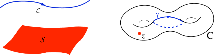
The six-dimensional perspective gives useful guidance in identifying and relating the various gauge theory observables. The (2,0) theory of type arises as the infrared limit of the world-volume theory of a stack of two coincident M-theory five-branes (together with a free 6d theory describing the center-of-mass motion). Each M5-brane contains a two-form potential with self-dual three-form field strength. An M2-brane can attach to an M5-brane via an open boundary, that sweeps out a 2d surface . It is a source for . The different ways of embedding inside the 6d space-time give rise to three different classes of gauge theory observables: (1) surface operators, (2) line or loop operators, and (3) point or ‘vertex’ operators:
-
1.
The surface operators are defined by considering an M2 boundary surface to be embedded111Although in this paper we mainly take , in the topological version of the theory one might consider more general space-time 4-manifolds and embedded surfaces , cf. [5, 6, 7, 8, 9]. in the 4d space-time and localized as a point on . In = 4 SYM theory, the surface operators are identified [7] as operators that create a singular vortex by allowing for a suitable singular boundary condition on the gauge and scalar fields along . For the most elementary class of surface operators, the vortex singularity is parametrized by two real parameters and ; here is the magnetic flux through the singular vortex and is a suitable 2d theta-angle. Both are naturally defined as periodic variables; from the M-theory point of view, they parametrize the location of the surface operator on .
As we explain below, a similar class of half-BPS surface operators can be defined in = 2 quiver gauge theories of interest. Moreover, for the most elementary class of such operators, the parameters () associated to the different gauge group factors can be glued together to specify a single location on the punctured Riemann surface .
-
2.
The line or loop operators are represented by M2-brane boundaries that wrap a one-cycle on , and extend along an infinite line or closed loop in . In the perturbative regime, where the surface decomposes into thin tubes sewed together via trinions, the loops labeled by the one-cycles around the thin tubes represent fundamental Wilson lines of the corresponding gauge groups. General Wilson-’t Hooft line operators can be thought of as the coupling of the gauge theory to the worldline of a dyonic point charge. The spectrum of possible Wilson-’t Hooft loops in the generalized quiver gauge theory is labeled by the set of closed non-selfintersecting paths on , up to homotopy [10]. As explained in [10], in a given weakly coupled description in terms of gauge theory with gauge group , this set has the physically expected form.
Line operators can act on surface operators, when the worldline of the former is embedded inside the worldsheet of the latter. The line operator then creates a discontinuity along in the parameters of the surface operator, generated by transporting its location on by the corresponding closed path on . Intuitively, we can think of this discontinuity as the effect of the generalized Dirac string of the dyonic point particle.
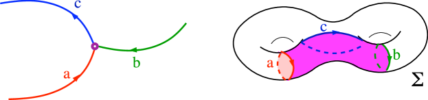
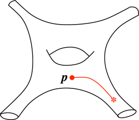
Figure 2: A point or ‘vertex’ operator may form a junction between several line operators. On , it spans an open region bounded by the (non-intersecting) one cycles associated with the line operators that meet at the junction. -
3.
Point or ‘vertex’ operators may form a junction between several line operators. On , they span on open region bounded by the (non-intersecting) one cycles associated with the line operators that meet at the junction. In the simplest case, when the boundary consists of three Wilson line operators in three adjacent gauge group factors, the point operator represents a point charge transforming in the corresponding trifundamental representation.
In this paper we will focus our attention on the surface and loop operators, and leave the study of the point operators for future work.
1.2 Computation strategy
We now summarize the basic strategy of our calculation of the expectation value of general Wilson-’t Hooft line operators on and . Although the validity of the actual computation does not rely on any unverified assumptions, it turns out that we can gain some useful geometric intuition by first stating the following conjecture:
The expectation value in the = 2 gauge theory of an elementary surface operator, specified by its position on , is equal to the Liouville CFT correlation function with the added insertion of a degenerate primary operator .
Although the complete proof of this conjecture goes beyond the scope of the present paper, in Sections 2 and 3 we present several pieces of evidence that support this proposed identification. For now, however, we will adopt it as a working hypothesis, that will help us formulate a practical procedure for computing the expectation values of Wilson-’t Hooft loops by means of the Liouville CFT correlation functions.
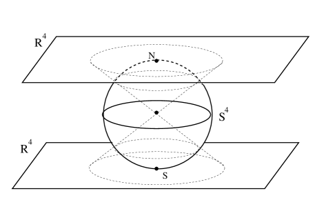
Let us state the conjecture a bit more precisely. As shown in [3], the Nekrasov partition function on is equal to a Liouville conformal block, i.e. a chiral half of the full Liouville correlation function, while the partition function on takes the form of an integral of the absolute value squared of a conformal block. So it is natural to identify the division of into the northern and southern hemispheres with the chiral decomposition of the Liouville CFT correlation functions into “left-moving” and “right-moving” chiral halves. To make this somewhat more concrete, imagine choosing hemispherical stereographic coordinates on as indicated in fig 3. The upper and lower halves of are projected on two copies of . We parametrize each by two complex coordinates and , such that the north and south pole of the project to the origin of the corresponding .
Now imagine adding a single elementary surface operator, inserted, say, on the lower copy of . In the gauge theory set-up of [11] and [4], there are two natural locations for the surface operators, namely and Both locations are invariant under the rotation symmetry used in the localization of the gauge theory path integral, which acts as
| (2) |
As we shall argue below, the expectation value of the simplest type of such surface operators located at corresponds to the insertion, inside the Liouville CFT conformal block, of a degenerate chiral vertex operator , while the same type of surface operators located at corresponds to the insertion of the chiral operator , which is the quantum version of the Liouville exponential . Indeed, these two types of surface operators are related by the symmetry . According to the dictionary of [3], in the Liouville theory it corresponds to switching the roles of and , which indeed relates the degenerate chiral vertex operators and . Note that the conformal block is multi-valued as a function of the position . This multi-valuedness arises because this class of surface operators on has an open boundary at infinity [7].
Via the hemispherical stereographic projection, the surface operator on can be thought of as the result of gluing together two “open” surface operators, one acting on the south copy of and one acting on the north copy of . We conjecture that the expectation value of the surface operator on is given by inserting a non-chiral vertex operator inside the non-chiral Liouville correlation function. Note that the non-chiral correlation function of is single valued as a function of , which is as one would expect for surface operators that do not have any open boundary. The factorization of the non-chiral operator into left- and right-moving chiral vertex operators amounts to splitting the closed surface operator into two “open” halves.
Next, consider a Wilson-’t Hooft loop labeled by a closed path on , acting on a surface operator on . For concreteness, we take the surface operator to be located at = 0, and the loop operator to act within the equator of the . The loop operator splits the surface operator into two open halves, glued together via a prescribed discontinuity in the parameters and of the singular vortex, i.e. via a jump in the location . Since the two sides correspond to the two chiral halves of the degenerate field , the discontinuity amounts to a relative shift in the location of the left and right chiral vertex operators by a full monodromy around . We can thus visualize the action of the Wilson-’t Hooft loop as performing a monodromy operation, in which one of the chiral vertex operators is transported along the closed path . This procedure is illustrated in fig 4.
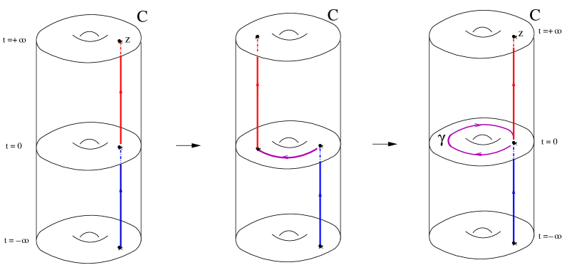
Finally, to get a Wilson-’t Hooft line in isolation, one can start by viewing it as the result of annihilating two identical surface operators, i.e. both are at the same location on and on , except that one of the two has a discontinuity as a result of acting with the given loop operator at the equator. Via the geometric visualization of the discontinuity as drawn in fig 4, we arrive at the identification of the Wilson-’t Hooft loop with the following familiar CFT monodromy operation:222 In the gauge theory, the four steps correspond to: (i) insert a “trivial” surface operator at = 0, (ii) split it into a pair of conjugate surface operators, each specified by the same parameter on , (iii) act with a loop operator on one of the two surface operators, (iv) let the two conjugate surface operators annihilate each other, leaving behind a bulk loop operator.
-
1.
Insert the identity operator inside the Liouville correlation function.
-
2.
Write as the result of fusing two degenerate Liouville operators , via their operator product expansion.
-
3.
Transport the chiral half of one of the two operators along the closed non-self-intersecting path that labels the Wilson-’t Hooft operator.
-
4.
Reconstitute the local operator (by recombining the two chiral halves), and re-fuse the two degenerate fields together into identity via the OPE.
The above monodromy procedure was introduced in the context of rational CFT by E. Verlinde [12], and played a key role in the derivation of the relation between modular transformations and the fusion algebra. It defines a linear operator, that acts non-trivially on the space of conformal blocks. To explicitly perform the various steps, one needs to know the modular properties of the conformal blocks under basic moves, known as fusion and braiding. Liouville field theory is a non-rational CFT, but its conformal blocks have rather similar modular properties as in rational CFT, except that the labels are continuous rather than discrete [13], [14]. In particular, the fusion and braiding matrices are known explicitly, and satisfy the necessary polynomial consistency relations. This knowledge is sufficient for us to turn the above four step procedure into a straightforward computation of the expectation value of the Wilson-’t Hooft line operators.
1.3 Organization
The rest of this paper is organized as follows. In Section 2, we set up a semi-classical dictionary between the =2 gauge theory and Liouville theory, based on the asymptotics of the Nekrasov partition function and the identification between the expectation value of the Liouville energy-momentum tensor and the quadratic differential describing the Seiberg-Witten curve. We pay special attention to the semiclassical behavior of the monodromies of the degenerate Liouville field .
In Section 3, we first recall the definition of the surface operators in the gauge theory, and provide an M-theory realization of them. We then present a semi-classical argument that supports their identification with the insertion of the degenerate fields in Liouville theory.
In Section 4, we consider the action of Wilson-’t Hooft loop operators on surface operators, and relate their expectation values to the monodromy of in the full quantum Liouville theory. As an application, we discuss how S-duality between the Wilson and ’t Hooft loops follows from elementary properties of CFT conformal blocks. In Section 5 we consider the Wilson-’t Hooft loop operators in the bulk, and use the recipe outlined above to compute their expectation value for the specific examples of and SYM theory. We briefly discuss their relation to observables on quantized Teichmüller space. We end with some concluding comments on open problems and future directions in Section 6.
In Appendix A and B, we have collected some useful facts about Liouville modular geometry, the form of the relevant fusion and braiding matrices and the relations among them. In Appendix C, we present an explicit calculation of the semi-classical limit of a degenerate operator insertion. Finally in Appendix D, we discuss the issue of self-intersecting paths on the Seiberg-Witten curve.
2 Semi-classical Liouville/gauge theory correspondence
In this section, we give a short overview of the semi-classical limit of Liouville CFT and its correspondence with the Seiberg-Witten solution of the class of = 2 gauge theories introduced in [2]. We then use this correspondence to study the semi-classical monodromies of the Liouville degenerate field .
2.1 Seiberg-Witten curve from Liouville
The IR dynamics of undeformed = 2 gauge theories on is completely characterized by the classical Seiberg-Witten (SW) curve. For our class of theories, the SW curve is given by the double cover of the Riemann surface , specified in terms of a quadratic differential defined on , as
| (3) |
has double poles at the marked points, whose coefficients encode the mass parameters of the gauge theory. The space of quadratic differentials with double poles of fixed coefficients is an affine space of dimension . This is also the dimension of the Coulomb branch. The Coulomb branch moduli of the field theory are identified with periods of the SW differential around a complete set of non-intersecting one-cycles on
| (4) |
The periods of the SW differential around the dual cycles on specify a dual set of parameters
| (5) |
The magnetic parameters are not independent from the , but determined via
| (6) |
where is the SW prepotential, which is an analytic function of the coupling constants and Coulomb branch parameters .
In the perturbative limit, there is a canonical choice of cycles which project to a complete set of mutually non-intersecting closed paths in the Riemann surface , that surround the thin tubes that characterize the gauge group factors of the generalized quiver gauge theory. The reader is warned this choice ceases to be canonical as soon as one moves away from the perturbative limit. The homology lattice of the SW curve is subject to all sort of interesting monodromies as one varies . At a generic point in the Coulomb branch, there is no preferred choice of a set of special coordinates .
To help compute the instanton partition sums of = 2 gauge theory, Nekrasov considered a deformation of the Lagrangian by two parameters and , both with the dimension of mass, that specify a certain rotation and some non-commutative modification of the space-time . This deformation breaks the translational symmetry and effectively places the functional integral on a compact space-time: the full partition function on is just a finite number , which depends meromorphically on the coupling constants and Coulomb branch parameters. Interestingly, coincides with a conformal block of the Liouville CFT defined on the base curve , with conformal fields placed at the punctures [3]:
| (7) |
Here, in our notation for the conformal block, we leave implicit the choice of pants decomposition of the Riemann surface . Both sides of this equality are given as a perturbative expansion in the instanton factors of the gauge groups, which are identified with the parameters of the “plumbing fixture” used to join the various pairs of pants. For example, when the base curve is a sphere, give the cross ratios of the coordinates of the insertions.333 There is a certain degree of arbitrariness in the precise definition of conformal blocks. Pairs of pants are glued together by a local coordinate transformation . The exact parameterization of the complex structure moduli space by the depends on the precise choice of a local coordinate at each puncture. Fortunately, the integration kernels implementing S-duality do not depend on the , and are thus insensitive to this choice. The instanton partition function suffers of similar arbitrariness, in the sense of some regularization scheme dependence. The ambiguity did not manifest itself in the explicit examples of [3], possibly because of an underlying brane construction.
In a sense, that we will make more precise in what follows, the Nekrasov deformation amounts to a “quantization” of the space of Coulomb branch parameters, that specify the SW differential of our class of theories. In accordance with this interpretation, we write444Note that this does not become the standard practice , at .
| (8) |
Here defines some mass scale, relative to which we will measure all other mass parameters. The parameter is related to the central charge of the Liouville CFT via with . The fields inserted at the marked points have Liouville momentum and conformal dimensions , where is the mass parameter for the flavor group associated to the -th puncture. The primary field propagating in intermediate channels is given by with
| (9) |
where is the Coulomb branch parameter, In other words, specifies the Liouville momentum in the channel.555In the following, we will refer to the exponent as the Liouville momentum. This operator has conformal dimension . The SW curve and associated prepotential emerges from the Nekrasov partition function in the “semiclassical limit” , or in 2d terminology, the limit where all Liouville momenta become large:
| (10) |
Here the canonical choice of -cycles is playing a hidden role. As both sides of (10) are defined by power series in the , the logarithm and the limit should be taken term by term in the expansion. The important monodromies of in the Coulomb branch are completely invisible to the expansion: each term is a rational function of the .
As was observed in [3], the quadratic differential that specifies the SW curve can be recovered in the semiclassical limit from the Liouville CFT, by considering the expectation value of the 2d energy momentum tensor
| (11) |
The quadratic differential defined this way has double poles at with coefficient given by times the conformal dimension , which in the semi-classical regime coincides with the squared mass parameter . Similarly, it is not hard to verify that the definition (4) of the parameters with the electric periods of the SW differential around the cycles, perfectly matches with the identification (9) with the intermediate Liouville momenta . Again, the match is to be understood term-by-term in the expansion.
It was shown by Pestun [4] that the instanton partition function of the undeformed gauge theory on is given by the integral over the Coulomb branch parameters of the absolute value squared of the partition function, with equal deformation parameters , where is the radius of :
| (12) |
This expression coincides with the partition function of the full non-chiral Liouville field theory. Since non-chiral CFT partition functions are invariant under modular transformations, this observation makes explicit that the partition function is S-duality invariant. In contrast, Nekrasov’s partition function on transform non-trivially under S-duality.
Indeed the conformal blocks labeled by different trivalent graphs can be considered as different delta-function normalizable bases of the same Hilbert space, labeled by the continuous parameters . The change of basis involves integration against an intricate kernel, which does not depend on the . If we denote the choice of trivalent graph for the quiver, or the conformal block, as , we can write schematically
| (13) |
where the are the complex structure moduli of the surface in the new basis.
2.2 Monodromies of the degenerate field
To gain more insight, it is useful to introduce the insertion of a degenerate local Liouville operator . As mentioned in the introduction, and explained in more detail in Section 3, we propose that this operator insertion corresponds to the gauge theory partition sum in the presence of an elementary surface operator.
Let us consider the properties of in the semi-classical limit. The degenerate field can be viewed as the operator with Liouville momentum equal to . It satisfies the relation , which implies that, when inserted in any correlation function, it satisfies a differential equation of the form
| (14) |
Here the normal ordering amounts to subtracting the double and single pole singularity as approaches .
For a general surface with punctures, the above differential equation has a large space of solutions, which one would like to identify with the space of conformal blocks with a degenerate insertion.666 The identification is true, but with an important caveat. The null vector decouples from correlation functions, but surprisingly does not decouple automatically from conformal blocks as well, unless one imposes “by hand” the degenerate fusion rule: the Liouville momenta on the two sides of the degenerate insertion must differ by . We will assume this constraint whenever we talk about conformal blocks with one or more degenerate insertions. A few more details are given in appendix B.1. The choice of sign in corresponds to the two solutions of the second order differential equation (14).
Since the conformal dimension of is fixed, and thus remains finite as , in the semi-classical regime one is allowed to replace by its expectation value (11). The semiclassical analysis of (14) thus is reduced to the WKB analysis of a holomorphic Schrödinger equation.
Consider the conformal block with a degenerate field insertion.
| (15) |
The insertion modifies the semi-classical limit (10) at subleading order, to
| (16) |
A basic WKB argument, combining (14) and (11), shows that
| (17) |
hence is (plus or minus) the integral of the SW differential along some path to the point , starting at some reference point :
| (18) |
The choice of sign in (18) corresponds to the two-fold degeneracy in the space of conformal blocks with a degenerate insertion.777As we will see in Section 3, in the gauge theory, the two fold degeneracy arises because the IR surface operators associated with a given gauge group factor have two degenerate vacua. We will denote the two WKB solutions by .
Since the SW differential has non-vanishing periods (4) and (5), (16) and (18) tell us that is a multi-valued function of the position of the degenerate field. As we will see later (and as detailed in appendix B.1), in the full quantum CFT this multi-valuedness is implemented via so-called fusion and braiding matrices, which in this case are given by matrices that relate the doublets of conformal blocks with the degenerate field inserted at different locations. The transport of along paths in the Riemann surface is implemented by the composition of a certain number of these matrices. We will denote the resulting transport operator along a path as .
As a crude first step towards finding the semiclassical behavior of , we could simply look at the monodromy of each WKB wavefunction. This monodromy depends on the periods of the SW differential along the lift of to the SW curve.888In the following intuitive argument, we will temporarily ignore some important structure associated to the fact that the same homotopy class in the base curve lifts to a multitude of possible homology classes in the SW curve. Still, the naive reasoning is rather instructive. The monodromy of the WKB wavefunctions around the -cycle on is given by a simple phase factor, determined by the corresponding Coulomb branch parameter999Here is a schematic notation for moving the position on along the cycle .
| (19) |
This behavior is as expected from standard CFT arguments: transporting a degenerate field around a certain leg of the conformal block produces a simple phase factor . This agrees at the leading order with (19).
The -cycle monodromy, on the other hand, takes the form
| (20) |
Via eqn. (6) and working to leading order in , we see that the prefactor in (20) can be naturally absorbed via a quantized shift in the Coulomb branch parameter associated with the dual -cycle:
| (21) |
Hence we see that the cycle monodromies may lead to shifts in the parameters by multiples of . We will confirm this fact via a more precise quantum treatment in Section 5.
As explained in the Introduction, the above monodromy operations represent the action of Wilson loops (for the monodromy) and ’t Hooft loops (for the monodromy) on a surface operator in the gauge theory. The above naive semi-classical expressions for these monodromies, while incomplete, already give some useful first hints at what general structure we should expect for the full answer.
First, we see that the conformal blocks with fixed parameters naturally form an eigenbasis of the monodromies of . The monodromies, on the other hand, act non-trivially on the eigenlabels . In the gauge theory, this corresponds to the fact that the instanton partition function (in the presence of a surface operator) on is an eigenfunction of the Wilson loop operator, while the ’t Hooft loop operator acts on the Coulomb branch parameters via quantized shifts.101010A priori, it may look somewhat surprising that the ’t Hooft loops can change the Coulomb branch parameters, and do not commute with the Wilson line operators. However, as noted earlier, the deformation effectively makes the space compact. Thus a localized operator may be capable of changing the vevs . Secondly, loop operators that act on a surface operator can be ordered in ‘time’; hence it is meaningful to talk about commutators between loop operators. S-duality can thus be thought of as a change of eigen basis from a set of ‘electric’ loop operators to some dual set of ‘magnetic’ loop operators.
Note further that the expectation value of a surface operator on , which is expressed as the integral over the Coulomb branch parameters of the absolute valued squared of the instanton sum, is a single-valued function of : the monodromies are phase factors that do not affect the norm squared, while the shifts in generated by the monodromies can be absorbed in a redefinition of the integration variables. This distinction between and expectation values is related to the fact that surface operators on are open (and thus may produce boundary terms upon partial integration), while on they are closed.
The above comments are all meant as intuitive expectations, based on a somewhat crude semi-classical arguments. The WKB approximation can be conducted in a rather more precise way, following the approach of [1]. A crucial step in [1] was a careful WKB analysis of a certain differential equation involving the same quadratic differential as we have here. This method can be applied with minor modifications to the holomorphic Schrödinger equation based on . The trick is to re-express the transport matrices for the differential problem as a linear combination of certain quantities , for which the naive WKB approximation along the path in the SW curve is correct. As detailed in appendix A of [1], is a linear combination, with integer coefficients, of , where the index runs over various possible lifts of to the SW curve. At different values of the parameters, different terms in the sum may be dominant in the semi-classical limit. Moreover, the integer coefficients which determine which is actually present in the sum are subject to discontinuous jumps as a function of the parameters. Only in a fixed perturbative limit, the naive WKB approximation around the cycles is valid. This is a rather degenerate case of the analysis in [1], where a maximal set of “closed WKB curves” emerges.
3 Surface operators in Gauge Theories
In this section we discuss a simple brane realization of half-BPS surface operators in gauge theory and argue that their counterparts in the low energy effective theory are labeled by points on the SW curve. Here we consider general gauge groups because our construction works equally well for any . We will restrict our attention to in Sec. 4 and 5, and compare gauge theory data with Liouville theory data.
As we will see, the brane construction shows that the twisted superpotential of the 2d theory on the surface operator is given by an integral along an open path on the SW curve , reproducing the formulae (16) and (18), thus supporting our identification between surface operators in the gauge theory side and insertions of degenerate operators in the Liouville side. We will also comment on how we can derive these results from the instanton counting in the presence of a surface operator.
Before we start, we should mention a relationship between our consideration of the surface operators and the analysis of quantum vortices in the Higgs phase of theories presented in the review [15] and references therein. There, supersymmetric Nielsen-Olsen type vortices were considered in the maximal Higgs branch of a specific theory, and the quantum dynamics of the zero modes living on the vortices was studied. They found a relation similar in spirit as (17), although they could only probe a very special point on the Coulomb branch, namely the root of the maximal Higgs branch. There is an obvious, sharp distinction between these vortices and our surface operators: the former are dynamical excitations of the theory, whereas the latter are operator insertions. Nevertheless, the two results are not completely unrelated. It is possible to consider a setup where an theory sits at the bottom of an IR flow initiated in a larger theory by a judicious Higgs branch expectation value. Vortex strings in the larger theory will flow in the far IR to surface operators: the magnetic fluxes of the low-energy gauge fields in the core of the vortex are squeezed to delta functions, and the tension of the strings goes to infinity. In a similar spirit, one can establish a relation between our surface operators in field theories, and the D-strings employed by [16] in string theory compactifications to give a physical interpretation to the refined open topological string amplitudes[17, 18].
3.1 Half-BPS surface operators
First let us recall the ultraviolet definition of surface operators. We are interested in half-BPS surface operators in gauge theories. The super-Poincaré subgroup preserving the surface operator corresponds to supersymmetry in two dimensions. More specifically, if we denote the two sets of 4d supercharges as , where denotes the eigenvalue of the Cartan generator of , the surface operator preserves a left moving half of and a right moving part of . This is motivated by the fact that we consider (mass deformation of) 4d superconformal theories, and the natural subgroup of the superconformal group which preserves a surface operator is
| (22) |
Four-dimensional multiplets restricted to the surface operator can be packaged into 2d superfields, useful to describe the couplings to the 2d defect. Different 2d supermultiplets can be identified with the help of the extra factor in (22), which commutes with the 2d superconformal group. The is a linear combination of the Cartan generator of and of the rotations in the plane transverse to the surface operator.
Abelian vector multiplets in four dimensions restricted to the surface operator yield a twisted chiral multiplet of charge under . Every such multiplet contains the 2d part of the field strength, together with the vector multiplet scalars. Twisted superpotential terms integrated over the surface operator will play a role which is quite parallel to the role of the prepotential in the 4d theory, as they are functions of the Coulomb branch vevs. Expanding in component, they give rise to couplings to the abelian 4d magnetic and electric fluxes across the surface operator.
For a surface operator that breaks the gauge group down to a subgroup (the so-called Levi subgroup [7]) one can introduce a 2d Fayet-Iliopoulos (FI) term of the form for each abelian factor in . A simple example corresponds to the next-to-maximal , e.g. (or ) in a theory with gauge group (resp. ). In this case, there is only one FI parameter , which can be conveniently written as in terms of real parameters and that have a simple interpretation in gauge theory [7]. Namely, the “magnetic” parameter defines a singularity for the gauge field:
| (23) |
where is a local complex coordinate, normal to the surface , and the dots stand for less singular terms. Note, in order to obey the supersymmetry equations, the parameter must take values in the -invariant part of , the Lie algebra of the maximal torus of .
On the other hand, the “electric” parameter enters the path integral through the phase factor
| (24) |
where
| (25) |
measures the magnetic charge of the gauge bundle restricted to . The monopole number takes values in the -invariant part of the cocharacter lattice, , which we denote as . The lattice is isomorphic to the second cohomology group of the flag manifold , a fact that will be useful to us later. Therefore,
| (26) |
and the character of the abelian magnetic charges takes values in , which is precisely the -invariant part of .
The “classical” twisted superpotential coupling on the surface operator which is associated to these surface operators is simply , where is the superpartner of , the restriction of the Coulomb scalar field to . On the Coulomb branch of the non-abelian gauge theory, the twisted superpotential will evolve into an effective twisted superpotential , a non-trivial function of the abelian Coulomb branch parameters. We propose that in general the effective twisted superpotential, much like the effective prepotential, is computable in terms of the SW curve . In particular, we claim that it is given by the integral of the SW differential along an open path (starting at some reference point ) on the SW curve,
| (27) |
The endpoint of the path provides an IR parameterization of surface operators.
Notice that in the IR abelian gauge theory, the superpotential is a function of the Coulomb branch parameters of the abelian gauge fields. The couplings to electric and magnetic fluxes live naturally in the Jacobian variety of the SW curve.111111More properly the Prym variety. For example in the case, the derivatives of the SW differential with respects of the parameters in produce holomorphic differentials which are odd under the involution of the ramified cover . Because the partial derivatives of the SW differential are, by definition, the holomorphic differentials on the SW curve, the map
| (28) |
coincides with the Abel-Jacobi map from a Riemann surface to its Jacobian.
3.2 Surface operators from M2-branes
Let us now study how these surface operators arise in terms of a surface operator in the six dimensional theory on a Riemann surface . In terms of M5-branes, this is a setup where M5-branes wrap in . The R-symmetry rotates the transverse , while the R-symmetry acts on the fiber of . The surface operator represents the endpoint of an M2-brane, stretched to infinity along a specific direction in . Therefore, the resulting surface operator is naturally labeled by a point in , when all the M5-branes are coincident and thus the theory is at the origin of the Coulomb branch.
In the Coulomb branch of the theory, the M5-branes merge into a single M5-brane wrapping the SW curve , an -ramified cover of in defined by an equation
| (29) |
Here are degree differentials on . The normalizable deformations of the correspond to the Coulomb branch parameters. The SW differential is . The M2-brane ends on the SW curve at a point .
As the abelian theory on a single M5-brane is well understood, we can understand directly the coupling of the surface operator to the fluxes of the 4d abelian gauge theory. The 4d fluxes are the components of the self-dual three form field strength on the M5-brane along the harmonic one forms on the SW curve. The surface operator couples to the self-dual three form field strength in a standard way: pick a three chain bounded by the surface operator and a reference surface and integrate the three form field strength along it. We reproduce the desired
| (30) |
and from that the twisted superpotential.
How should we understand the relation between the UV label and the IR label ? The degrees of freedom living at the UV surface operator appear to have distinct vacua in the IR. We would like to interpret the SW equation as a chiral ring relation for a twisted chiral superfield , capturing the dynamics of such degrees of freedom. At least locally, if we consider a small variation of the 2d coupling , it is natural to consider as an FI parameter for the twisted chiral superfield .
The twisted chiral superfield resembles closely the generator of the quantum chiral ring of a sigma model. This is not a coincidence. The basic surface operators in the gauge theory, which break the gauge symmetry to the subgroup , have a natural relation to a sigma model: one can always re-instate full gauge symmetry on the surface operator by introducing a compensator field living in . This compensator field may well become dynamical in the IR.
A weakly coupled gauge group in four dimensions arises from the M5-brane theory whenever a tube in the Riemann surface is close to degeneration, i.e. becomes long and thin. In this limit the theory along the tube can be reduced to a 5d Yang-Mills theory in a segment, and then to a weakly coupled 4d gauge theory. The gauge coupling is the modular parameter of the tube. If the M2-brane is attached to (one of) the M5-branes in the long tube region, it will clearly produce a defect in the 4d gauge theory which breaks to .
We can be more precise. As we reduce from the theory on a long, thin tube to a weakly coupled 5d Yang-Mills theory on a long segment, the M2-brane surface operator descends to a D2-brane surface operator, represented in the 5d theory by a ’t Hooft monopole operator of minimal charge. The position of the original puncture on the M-theory circle is encoded in the angle coupled to the magnetic flux integrated over the surface operator. By supersymmetry, the holomorphic coordinate along the tube must coincide with the holomorphic combination . We still have to fix a reference point, , that will be discussed below.
To summarize, we conclude that the definition of standard surface operators in SYM theory can be easily extended to surface operators in theories in the weak coupling regime, provided that the punctures are well inside the tubes of the Riemann surface. As the puncture moves through pair of pants from one tube to another, the corresponding surface operator must undergo some interesting 2d duality transformation.
To understand better the detailed structure of the surface operators, we will follow a standard route [2]: we will first focus on a subclass of theories, the conformal linear quivers of unitary groups, which have a brane realization in IIA theory [19].
3.3 Brane construction in type IIA
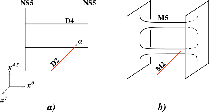
Let us consider a stack of D4-branes intersecting NS5-branes. We take the NS5-branes to be along the directions , , , , and D4-branes to be along the directions , , , , and . This setup realizes a conformal linear quiver of groups, with fundamental hypers at each end. In M-theory, it lifts to a brane configuration which we identify with the theory “compactified” on a cylinder, with simple defects.
To produce transverse, semi-infinite M2-branes in the M-theory setup we need transverse, semi-infinite D2-branes in the IIA setup. They should preserve half of the remaining supersymmetry of the D4 and NS5 brane system. We choose the D2-brane worldvolume to be along the directions , , and , as in Figure 5 . Below we summarize the worldvolume directions of various branes in the resulting configuration:
| NS5 | (31) | |||
| D4 | (32) | |||
| NS5′ | (33) | |||
| D2 | (34) |
where we included a new kind of the five-brane, denoted as NS5′, with worldvolume along the directions , , , , , and . The NS5′-brane preserves the same part of the 4d supersymmetry as the D2-brane and is useful for identifying the half-BPS surface operator represented by the D2-brane.
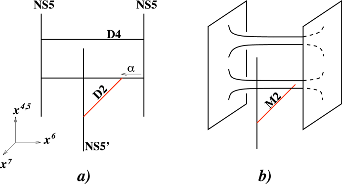
In the presence of the NS5′-brane, the D2-brane can have a finite extent in the direction by stretching between the NS5′-brane on the one end, and the original system of D4 and NS5 branes, on the other, as illustrated on Figure 6 . When the D2-brane has finite extent in the direction, its worldvolume theory is effectively a 2d gauge theory with the coupling constant
| (35) |
In particular, the original brane configuration on Figure 5 can be recovered in the limit , which corresponds to the weak coupling limit of the D2-brane theory.
To be precise, it is convenient to start by attaching the D2-brane to one of the NS5-branes. The Neumann boundary conditions on the D2-brane worldvolume theory allow for a simple dimensional reduction to a 2d gauge theory. The effective theory on the D2-brane is supersymmetric gauge theory with gauge group and a certain matter content, which is easy to read of from the brane construction on Figure 6 . Specifically, we have the following theory in two dimensions (with space-time coordinates and ):
Indeed, up to a simple change of coordinates, this setup is related to the brane system considered in [20] that engineers 2d abelian gauge theory with chiral multiplets of charge . In the D2-brane theory, the boundary conditions corresponding to the NS5 and NS5′ branes project out all massless string modes, except for a vector multiplet. Indeed, since the NS5-brane is localized in the directions , , , and since the NS5′-brane is localized in the directions , , , , the D2-brane can only move along the directions and (which are common to both the NS5 and NS5′ brane). These two modes combine into a complex scalar field on the D2-brane worldvolume,
which can be identified with a complex scalar in the 2d vector multiplet (equivalently, twisted chiral multiplet).
Once we have D2, NS5, and NS5′ branes, incorporating the D4-branes does not break supersymmetry further. The D2-D4 open string states give rise to charged chiral multiplets (one for every D4-brane) resulting in the effective theory (3.3). Note that, in the D2-brane theory, the vevs of the 4d adjoint scalar field play the role of twisted mass parameters and the gauge symmetry of the 4d gauge theory on the D4-branes plays the role of the flavor symmetry. For generic values of the flavor symmetry is broken to a subgroup . We get a set of chiral multiplets of charge from the D4-branes ending on the left of the NS5-brane, and a set of chiral multiplets of charge from the D4-branes ending on the right of the NS5-brane.
These 2d fields couple in a standard way to the 4d gauge fields arising from the D4-branes, and also couple (via cubic superpotential) to the bifundamental adjoint hypermultiplets coming from the D4-D4 strings (stretched between the two sets of D4-branes). Giving expectation values to the bifundamental fields corresponds to reconnecting the D4-branes and separating them from the NS5-brane; this operation is known to give a mass term to the 2d chiral multiplets [20].
Now, let us turn on a parameter that corresponds to moving the NS5′-brane (and, therefore, the D2-brane) in the direction. It forces the D2-brane to end on one of the D4-branes, cf. Figure 6 . From the point of view of the 2d theory on the D2-brane it corresponds to turning on the Fayet-Iliopoulos parameter of the gauge group [20]. Depending on the sign of the FI term, either the chiral fields of charge or of charge gain expectation values, connecting the D2-brane and either set of the D4-branes. To match the brane picture, it must be the case that the cubic superpotential coupling will insures that only one of the two types of fields can receive expectation values. Indeed an expectation value for both types of fields would act as a delta-function source for the four dimensional hypermultiplet fields. In the Coulomb branch of the theory, expectation values for the Higgs branch fields, which are massive, will typically break SUSY.
If all the parameters are set to zero, the space of vacua in such a theory is the Kähler quotient
The Kähler modulus can be combined with a B-field on the target space to a complexified FI parameter . In 2d theories, such as the one we are considering, the values of the Fayet-Iliopoulos parameter and the theta-angle are renormalized due to quantum corrections. The renormalized value of the complex parameter can be expressed in terms of the twisted superpotential:
| (36) |
As was explained above, in the brane construction the classical (“bare”) FI parameter is identified with the position of the D2-brane in the direction, cf. Figure 5 , while its “quantum” companion can be identified with the position in the direction (which is not manifest in the type IIA theory/classical field theory). As in [19], we can describe quantum corrections by performing the usual M-theory lift of this picture and identifying the effective value of the complexified FI parameter in the IR theory with the distance between the M2-brane and the M5-brane in the complex plane parameterized by ,
| (37) |
Combining this with eq. (36), the identification of the position in the plane with the twisted chiral field , and the fact that the M5-brane worldvolume is the SW curve , we arrive at the following property of the twisted superpotential:
| (38) |
This expression is actually equivalent to (27). Indeed, eq. (27) represents the effective superpotential for the bulk fields after integrating out . By the standard rules of the Legendre transformation, the solution to (38) is the derivative of the effective superpotential with respect to , i.e. .
The linear sigma model construction we meet here has some interesting features, and an unpleasant one. On the one hand, it gives a slightly better definition of surface operators than the one based on a codimension two singularity for the gauge field, or the coupling of the 4d gauge theory to a sigma model on . The advantage of the linear sigma model is that it allows one to follow the “flop” from positive to negative values of , which appears to relate surface operators for consecutive gauge groups in the quiver. On the other hand, it is still not as powerful as one might desire: e.g. in the case, where the flavor symmetry of the bifundamental field is promoted to a crucial flavor group, one has to gauge this symmetry group to produce a generalized quiver. The cubic superpotential coupling of the bifundamental field (in the example, an “trifundamental”) to the 2d chiral multiplets cannot preserve this extra symmetry.
It would be interesting to find a description of the surface operator capable to describe in a symmetric fashion all three possible “flops” which may transport the basic surface operators of either of the three groups through the pair of pants.
We have now a rough, self-consistent picture of the correspondence between six and four dimensional surface operators, in a given weakly coupled four dimensional Lagrangian description. Well inside a tube the surface operator should be well described by the basic defect operator where the gauge group corresponding to the tube is broken to a subgroup. Near the endpoints of the tube, the pure gauge theory description breaks down, and the defect is better described by coupling to a 2d sigma model, associated to a specific pair of pants. Flops in the 2d sigma model connect the surface operators living on different legs of the pants. We will not attempt to refine this picture further in this paper.
3.4 Instanton counting
Now we are ready to discuss instanton counting in the presence of a surface operator. In particular, our goal is to clarify the claim, made in the previous sections, that the semiclassical behavior of the Nekrasov partition function in the presence of a surface operator121212It is worth noting that in [21] it has been independently proposed that the instanton partition function in the presence of a surface operator should satisfy a differential equation of the type (14). It would be interesting to explore further the connections with that work. matches the semiclassical limit of the conformal block with the insertion of a degenerate field, and to set the stage for a computation beyond the semiclassical limit (that we will not attempt in the present paper).
Following [11], we introduce the generating function
| (39) |
where and is the moduli space of “ramified instantons.” From the point of view of the 4d gauge theory (where a surface operator supported on is defined as in (23) and (24)) the ramified instantons are anti-self-dual gauge connections on with instanton number and monopole number .
As noted above, one can also represent surface operators of Levi type by studying 4d gauge theory on coupled to a 2d sigma model on with the target space . In this description, the complex parameter is the complexified Kähler modulus of the flag manifold and “ramified instantons” with can be thought of as the usual instantons of the 4d gauge theory combined with 2d worldsheet instantons of the sigma model. Indeed, according to (26), the monopole number measures the degree of the map . In the case we are mostly interested in, where is the next-to-maximal Levi subgroup, we have and the monopole number is simply an integer, .
The moduli space is non-compact, so the integral in (39) needs to be properly defined (regularized). This can be achieved by noting that admits a natural action of the gauge group (which acts by a change of framing at infinity) and an action of the 2d torus (induced by the action of on ). Therefore, the integral on the right-hand side of (39) can be conveniently regularized by considering the equivariant integral of the unit -cohomology class over . This integral takes values in the field of fractions of the ring , which can be identified with the ring of functions on the Cartan subalgebra of , invariant under the Weyl group. Therefore, the equivariant integrals on the right-hand side of (39) are rational functions of , , and , where and denote coordinates on the Lie algebra of and , respectively.
As in [11], combining the instanton partition function with the classical term and the one-loop term we obtain the full partition function,
| (40) |
that we already encountered in Section 2. As we claimed there, the general structure of conformal blocks with degenerate field insertions match the semiclassical expansion of the partition function in the presence of surface operators,
| (41) |
where the prepotential and the twisted superpotential are the F-terms of the 4d theory on and the 2d theory on that contribute to the Nekrasov partition function. Indeed, by the localization rule
where we assumed that the surface operator is supported on a plane . For a surface operator supported at the roles of and are exchanged. As we explained in Section 2, in the Liouville theory these surface operators correspond to the degenerate fields and .
Notice that the surface operator breaks the permutation symmetry between the . In particular, the classical twisted superpotential will be written as for a certain choice of . More generally, the instanton partition function is not invariant under Weyl group permuting the , unless one acts on this extra dummy label as well. This is as it should be to match the conformal block interpretation. Conformal blocks without a degenerate insertion are labelled by continuous (Liouville or Toda) momenta, each subject to the identification by the action of the Weyl group ( for Liouville theory). Conformal blocks with a degenerate insertion in a certain leg carry an extra discrete label: the momenta on the two sides of the degenerate insertion must differ by a value allowed by the degenerate fusion rule. The Weyl group acts non-trivially on this difference. This discrete label coincides with the extra dummy label in the instanton partition function.
More generally, we believe that, for every conformal block with a degenerate field insertion, there should be a half-BPS surface operator supported on a surface invariant under the symmetry (2). The definition of such surface operator should be given in the corresponding generalized quiver gauge theory, and allow for a computation of the Nekrasov partition function in the presence of the surface operator. In particular, it is natural to expect that the degenerate field corresponds to a surface operator supported on a degenerate curve defined by the equation .
4 Line operators on surface operators
theories in two dimensions have interesting half-BPS line operators. They preserve the diagonal combination of . A useful way to produce such line operators is to consider a deformation of the theory where some marginal coupling has a non-constant profile as a function of the space coordinate over a finite region . A flow to the IR sends the scale and squeezes the profile to a step function.
The resulting line operators are labeled by the path in the space of couplings, up to homotopy. This construction applies as well to the construction of line operators inside surface operators. A simple, rich example appears in [7] in the case of super Yang-Mills. We are especially interested in line operators for which the path in the space of couplings is closed, so that the line operator does not interpolate between two distinct surface operators.
It is easy to understand the meaning of such line operators in an Abelian gauge theory. If we consider a profile for the coupling to the magnetic flux, and we write with , we get a term in the Lagrangian
| (42) |
In the IR the latter term reduces to . (We take the surface operator to span ). This line operator coincides with the insertion of a Wilson line for the gauge group! A similar reasoning (or a simple electromagnetic duality) shows that a discontinuity coincides with the insertion of a ’t Hooft line operator.
We can use this result in two ways. In a non-Abelian gauge theory where the surface operator breaks the gauge group to, say, , the Wilson and ’t Hooft line operators will live in the factor. These operators are defined independently from the bulk line operators. However we will learn how to reproduce the bulk line operators from line operators living on a surface operator.
In the Coulomb branch of the non-abelian gauge theory, the line operators will take the form of ’t Hooft-Wilson line operators with charges . As the parameter space of surface operators in the IR coincides with the SW curve , one could consider line operators in the IR associated to a closed path on , which carry charge
| (43) |
Alternatively, in a canonical basis of one-cycles.
From the six-dimensional point of view, as our surface operators are labeled by a point in the curve over which the twisted theory lives, we expect to see line operators labeled by closed paths in , up to homotopy. We have two rather distinct ways to label a line operator attached to a surface operator: a homotopy class of paths in in the UV 6-dimensional theory, and a homology class in in the IR theory. We already encountered this phenomenon in Liouville theory, and understood the relation to the WKB analysis of [1]: expectation values of UV line operators are linear combinations of individual contributions, each taking the form expected from an IR line operator.
Now we are ready to provide explicit expressions for the 2d CFT operators which represent the action of line operators on surface operators.
4.1 Line operators from braiding and fusion
In order to introduce line operators in a setup where localization is possible, we need the support of the line operator to be invariant under the two relevant isometries. The isometries are the rotation in the plane of the surface operator, and the rotation in the plane orthogonal to the surface operator. Although until now we mostly referred to straight line operators, a conformal transformation allows us to consider circular line operators as well. In complex coordinates on , we can consider a surface operator at with a line operator at . The same location works for , in stereographic coordinates.
Given a conformal block with the insertion of a degenerate field , we can ask: what is the effect of transporting the point along a closed path on the surface ? This is a well studied problem in the context of rational conformal field theories [22]. If we insert the operator in a certain channel of the conformal block, the result is (by definition) a power expansion in , which is convergent as long as lies in the corresponding tube of the Riemann surface. The conformal block is defined outside that region by analytic continuation. The analytic continuation is naturally executed stepwise, by moving from a tube to an adjacent one. Such elementary moves are represented by matrices acting on the corresponding spaces of conformal blocks. We refer to Appendix B for a discussion of this fact, and a review of the explicit calculation of the fusion and braiding matrices.
In order to understand the elementary moves, we just need to consider the simplest possible setup, where a single degenerate insertion moves between the three legs of a three-point vertex of full punctures. This has the physical interpretation of a surface operator in the “pair of pants” theory of four free hypermultiplets, with masses turned on in the Cartan of the flavor subgroup.
If we place the full punctures of Liouville momenta respectively at ,, on the sphere, and the degenerate insertion at , the conformal blocks can be given explicitly in terms of hypergeometric functions. The basis of conformal blocks where the degenerate field is inserted, say, on the leg behave as as . The transformation of basis to solutions with well defined behavior near is called fusion matrix, and will be denoted as . This has to be intended as a transport along the positive real axis. The transformation of basis to solutions with good behavior as is called braiding matrix, and will be denoted as . The sign refers to transport from to along the positive real axis, on either side of .
For more general conformal blocks, we need to set up a useful convention to distinguish the continuous labels at the intermediate channels from the discrete label associated to the shift. In order to do that, we add a dummy label to the conformal block: we do not just specify in which leg of the conformal block we insert the degenerate field, but also “near which end” of the leg. Thus we label the conformal block by the Liouville momentum through the “long” piece of the leg. The other, “short” part of the leg has momentum . When a degenerate insertion is moved from one end to the other of the same leg, the notions of “long” and “short” parts of the leg are exchanged, and the continuous label is shifted by .
The transport of the degenerate insertion along a path in the Riemann surface gives a sequence of elementary operations:
-
•
fusion and braiding matrices, which only act on the discrete label
-
•
transport along a leg, which act by a diagonal shift operator
-
•
transport around a leg, which provides a diagonal phase factor.
It is rather simple to connect this decomposition to the semiclassical approximation in the perturbative regime. In that regime, the branch points of the cover lie in the pair of pants regions, away from the long, thin tubes associated to the gauge groups. It is easy to see from the expression of for the pair of pants theory that each pair of pants in supports a single cut in the branched cover . Only when the path in passes through a pair of pants there is some ambiguity on the lift in . The fusion and braiding matrices differentiate between the two possible choices of sheet of entering and exiting the pair of pants. The transport along and around the tube is perfectly diagonal, and well described by the naive WKB analysis.
4.2 S-duality of line operators in theory
As an illustrative application of the Liouville CFT technology, let us consider the loop operators, acting on a surface operator, in gauge theory, for which the instanton partition function coincides with the Liouville conformal blocks of the four punctured sphere. As usual, we place the punctures, of momenta ,,, respectively at , and consider a trivalent graph connecting and by a channel of momentum . We will now introduce the Wilson and ’t Hooft loop operators via the CFT monodromy operation, and explicitly demonstrate that S-duality interchanges the two.
The surface operator is represented by a (2,1) degenerate operator placed at some location on one of the legs of the conformal block. For definiteness, we place it on the internal leg of the conformal block, say, near the vertex. As will become clear below, this choice is particularly convenient for studying the action of S-duality.
The basic Wilson line operator transports the degenerate field around the internal leg. In the notation of the appendix B, this produces a simple phase factor
| (44) |
To do S-duality, we need to apply a fusion matrix that maps the original ‘s-channel’ conformal block into a ‘t-channel’ block, associated to a graph where and are joined by an internal leg of momentum . If, during this operation, we want to keep the degenerate field insertion in the intermediate channel, we need to specify in detail the relative motion of the punctures at and . It is simpler to move away from the intermediate leg, and place it, say, on the external leg. With this choice, the Wilson line operator takes the schematic form
| (45) |
the degenerate insertion is transported (via a fusion matrix ) to the intermediate leg, rotated around it via , and then fused back to the external leg (see Fig. 8).

A priori, we could now compute the ’t Hooft loop expectation values by defining them as the Wilson loops in the S-dual theory, and by using the known form of the fusion matrix that implements the S-duality transformation on the Liouville conformal blocks:
| (46) |
In other words, the ’t Hooft loop could be obtained by commuting the Wilson loop with
| (47) |
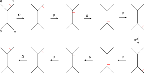
However, the fusion matrix for arbitrary conformal blocks is quite involved, and this type of calculation is hard to do in practice. So instead, we define the ’t Hooft loop more directly, via the monodromy operation of a degenerate field on the S-dual path, as indicated in fig 9. Schematically, the sequence of moves that defines is (c.f. fig. 9):
| (48) |
the degenerate insertion is rotated to the other side of , fused to the internal leg, transported across it, rotated around , transported back, fused back to the external leg, and rotated to the original configuration. Because of the two shift operators, the final expression contains three different terms, where is subject to shifts .
The monodromy operation in Fig. 9 involves relatively simple braiding and fusion matrices, that do not act on the modular parameter , that defines the gauge coupling. Moreover, the braiding and fusion matrices can be shown to satisfy important consistency relations, known as the pentagon and hexagon identities, which among others can be used to derive the S-duality relation (47). The relation is proved graphically in Fig. 10.
Here we sketch the algebraic steps. First, we expand: . We apply the pentagon identity to the block in parenthesis and commute through . Another pentagon identity and commutation brings us close to the final result . Finally, two hexagon relations give .
5 Line operators
We are now ready to study the gauge theory line operators that act in the bulk, without any (nearby) surface operators. Such bulk line operators a priori look quite different from the line operators that act on a surface operators. Surface line operators are essentially abelian, since (for a surface operator with a next-to-maximal Levi subgroup) they live in a single factor of the gauge group , whereas bulk line operators are non-abelian. Nonetheless, we claim that a bulk line operator can be obtained by annihilating two identical surface operators, one of which contains a surface line operator.131313To see this, recall that a surface operator restricts the gauge transformations to the subgroup that, at the surface, commutes with the . Annihilating two surface operators reinstates the full gauge symmetry. The bulk loop is given by averaging the surface loop over the full gauge orbit. Via standard coadjoint orbit quantization, this yields a non-abelian loop operator. In the Introduction, we used this insight, combined with the 6d perspective, to argue that the Wilson-’t Hooft loops in our class of gauge theories can be identified with certain loop operators in Liouville CFT, defined in terms of the four step monodromy procedure summarized in Section 1.2. In this section, we will use this identification to compute the expectation values of Wilson and ’t Hooft loops for certain basic examples. First, we will present an independent motivation for our proposed CFT definition of the line operators.
5.1 Wilson-’t Hooft loops from Liouville CFT
Consider a circular Wilson line in the spin representation of the -th gauge group factor. As shown by Pestun, inserting inside the gauge theory instanton sum on , i.e. with given Coulomb branch parameters , simply amounts to multiplication by the corresponding character
| (49) |
Here and in the following, the summation for the half-integral stands for the sum over half-integral between and . Instanton sums on are therefore eigenfunctions of the circular Wilson line operators. On , the Wilson loop expectation value takes the form
| (50) |
A similar direct gauge theory calculation of the expectation value of ’t Hooft loop operators in gauge theories is not yet available. However, based on the semi-classical discussion of section 2, we expect that these will take the following schematic form
| (51) |
where denotes some ’t Hooft loop associated with the spin representation. In the following we will explicitly compute the kernel in some specific examples.
The Wilson and ’t Hooft loops are special cases of a more general class of dyonic ’t Hooft-Wilson line operators, whose systematic study was initiated in [23, 24]. We can make contact here with the recent work [10], which provides a useful classification of ’t Hooft-Wilson line operators in generalized quiver gauge theories. The operators are labeled by a set of magnetic and electric charges and for each gauge group, subject to an identification for each , and to a constraint: the sum of the three magnetic charges for the three gauging a single matter block should be even.141414The authors of [10] find it useful to enlarge the space of line operators, by including magnetic flavor line operators. Here, for now, we only consider line operators for the gauge groups. The authors of [10] propose a suggestive identification between the set of line operator charges and the set of (homotopy classes of) closed non-selfintersecting curves in C. This classification via closed non-selfintersecting paths on naturally fits with the description of the loop operators via the 6-d (2,0) theory as the end-point of supersymmetric semi-infinite M2-branes, as reviewed in the Introduction.
Correspondingly, we will denote a general Wilson-’t Hooft loop operator by
| (52) |
Here the label indicates the spin of the representation. In the gauge theory, the operators can be thought of as the effect of transporting a dyonic point particle, with charge labeled by the path , around the loop trajectory.
In a given perturbative regime, one can identify a complete set of non-intersecting cycles on , that lift to a complete set of -cycles on the SW surface . We will denote this set of cycles by . On the SW surface, we can choose a set of dual -cycles, that project back to to a set of dual cycles that we denote by .151515This description is slightly oversimplified. The and -cycles lie on the Prym curve of . Moreover, the set of B-cycles is not unique. E.g. one is free to apply shifts of the form . In the gauge theory, this freedom is a reflection of the Witten effect, shifts in the dyonic charge spectrum by one electric unit. For small theta angles , however, there is a preferred choice of dual B-cycles that correspond to the pure monopole charges. The Wilson and ’t Hooft loops are then identified as the loop operators associated with the A and B-cycles, respectively
| (53) |
If one would consider the insertion of multiple Wilson lines (all located on concentric circles, invariant under the rotation that is used to justify the localization of the gauge theory path integral), one would discover that the Wilson lines form a commutative and associative algebra, given by the representation ring of :
| (54) |
Via S-duality, we thus learn that, in general, all operators associated with some given path form a commutative associative algebra, isomorphic to the representation ring. More generally, we will see that two line operators and do not commute in case the two curves and intersect.
We now set to describe the identification between line operators of charge and the Verlinde loop operators associated with the same path on .161616In fact, we face a small puzzle here: as we will see shortly, the loop operators in the CFT make sense for all , while the gauge theory line operators appear to require the loop to be non-self-intersecting. We will propose a resolution to this puzzle in Appendix D. Within the context of rational CFTs, the Verlinde operators are known to generate a commutative and associative algebra, given by the fusion algebra of the CFT. Here we would like to define analogous operators in Liouville theory.
Liouville CFT is a non-rational CFT. It has a continuous spectrum of primary operators. Furthermore, part of the operator spectrum, including the identity operator, create non-normalizable states. It is not at all obvious, therefore, that Liouville theory possesses a well-defined fusion algebra, with similar properties to that of a rational CFT. However, the discrete sub-spectrum of degenerate Virasoro representations do seem to specify a well-defined closed sub-algebra. In particular, the Virasoro modules associated with the operators generate a closed fusion algebra
| (55) |
This algebra is identical to the representation ring of , via the identification More generally, the fusion algebra of a degenerate field with a continuous representation also seems well defined. It reads (here )
| (56) |
where denote the chiral sub-Hilbert space with given Liouville momentum . Here and in the following, the symbol for (half-)integral stands for the summation over as usual.
We now define the Verlinde monodromy operators via the following recipe [12]:
-
1.
Insert the identity operator inside a chiral Liouville correlation function.
-
2.
Write as the result of fusing two chiral operators , via their OPE.
-
3.
Transport one of the operators along a closed non-self-intersecting path .
-
4.
Re-fuse the two degenerate fields together into identity , via their OPE.
This procedure defines a linear map on the space of Liouville conformal blocks. We need to introduce a normalization factor in order for these operations to represent the fusion rule [25]. We will come back to this point shortly.
As a concrete illustration, let us consider the simplest case of SYM theory, corresponding to Liouville theory on the torus. The genus 1 conformal blocks are given by the chiral partition sum, defined by the trace of over the sub-space
| (57) |
with . These conformal blocks span a linear space, on which the monodromy operators act. The monodromy operators around the A-cycles manifestly act diagonally, via eigenvalues that generate the representation ring, and thus are naturally given by (specialized) characters. One finds
| (58) |
with as given in eqn (49). This establishes the identification of with the Wilson line operators . The action on the conformal blocks generated by the monodromy around -cycles should reflect the fusion algebra of the corresponding degenerate field [12, 25]. Indeed, one finds that
| (59) |
These operators also generate an representation ring. Since S-duality interchanges the and -cycle, we identify with the ’t Hooft loop. Note that the S-duality map amounts to taking a Fourier-transform, or equivalently:
| (60) |
This relation matches with the results of the semi-classical study in section 2. It is important to note, however, that it is special to the case of SYM theory; in general, the S-duality transformations are much more involved, as we will see shortly.
We should note here that, to obtain the above results, one needs to apply a standard normalization factor such that the operator associated with the -cycle, when acting on the identity representation, produces the degenerate character with unit pre-coefficient with The required normalization factor depends on , but is otherwise the same for every path . To compute the factors , we perform the monodromy operation
|
|
For the first two degenerate insertions under consideration we obtain and In general we expect to find Upon multiplying the ‘bare’ CFT monodromy operators by this factor, we get the properly normalized Verlinde operators , that are identified with the ’t Hooft-Wilson loop operators.
In the following we will consider examples of Wilson and ’t Hooft loops in the simplest gauge theories, namely and with four flavors.
5.1.1 Example 1: Wilson loop in
As a first concrete check, we now compute the Wilson line in the gauge theory with fundamental flavors, corresponding to the four punctured sphere.
For simplicity, we first focus on the spin 1/2 representation, defined by the monodromy of the degenerate field . It generates the fusion algebra
| (61) |
According to our previous discussion, we define the Wilson loop by the operation:
|
|
(62) | |||
| (63) | ||||
| (64) |
For details on the notation, see Appendix B. The degenerate fusion rules imply that the momentum of the intermediate channel of the first and last graph is , which we shortly denote by . Notice that the channel corresponds to the state with zero momentum. The Wilson loop is then
| (65) |
The correct expressions for the fusion and flip matrices can be found in Appendix B. Performing the explicit computation gives
| (66) |
As already mentioned, once the fusion matrices with a degenerate insertion are given, we can use the pentagon and hexagon identities in order determine the fusion matrices with a degenerate insertion . Via this route, we have computed the fusion matrices with a degenerate insertion. We obtain for the corresponding Wilson loop The general answer can now be guessed, and agrees with the gauge theory result (49)
| (67) |
Note that, since the monodromy calculation can be performed locally on a given internal leg of the conformal block, this result for the gauge theory with flavors is sufficient to fix the form of any Wilson line in any member in our class of gauge theories. The precise match between (67) and (49) formed the original motivation for our proposed identification of the Wilson-’t Hooft loop operators with the Verlinde operators. Combined with the geometric motivation presented in the Introduction, based on the relation with surface operators, this precise match can be viewed as direct evidence supporting the conjectured identification between surface operators and degenerate operator insertions in the Liouville CFT.
5.1.2 Example 2: ’t Hooft loop in
We now turn to the ’t Hooft loop of the theory, corresponding to the torus with one puncture. It is specified by the following monodromy operation:
|
|
(68) | |||
| (69) | ||||
| (70) |
Note that in the last line, there are two types of terms: one has and has the vacuum in the fusion of the two degenerate states with ; the other has and has in the fusion of the two states with . As we did for the case of the Wilson loop, we project on the term which has the vacuum in the fusion. We can write the result in the following form
| (71) |
Note that the full operation again involves shift operators of the form .
In terms of the fusion and braiding matrices
| (72) | ||||
| (73) |
Finally, using the explicit expression for and we obtain
| (74) | ||||
| (75) |
Here the mass parameter is normalized so that at the theory reduces to SYM theory, i.e. corresponds to inserting the identity operator at the puncture.
A consistency check
The Wilson loop operator is “hermitian,” in the sense that inside a full correlation function on one can act with the Wilson line either on the holomorphic or the anti-holomorphic conformal block, and obtain the same result: indeed the Wilson loop operator (50) is diagonal in the integration variable , and symmetric under . For consistency, the ’t Hooft loop should satisfy the same constraint.
Up to the usual normalization factor, the integral expression for the expectation value of the ’t Hooft loop is (here )
| (76) |
where denotes the DOZZ three point function. The DOZZ pre-factor arises as a one loop determinant in the gauge theory, and does not depend on the gauge coupling. The conformal block represent the sum over the classical instanton contributions, and do depend on the gauge coupling. For the case, the partition function on further simplifes and reproduces the semi-classical calculation on the gauge theory side performed in [26]; for details, see Appendix E.
For the DOZZ three point function takes the form
| (77) |
The action of the ’t Hooft loop is non-diagonal in the integration momentum . Hence to compare the action of the ’t Hooft loop on the holomorphic conformal block and the action on the anti-holomorphic conformal block one needs to shift the integration contour, taking into account the effect of the shift on the relevant DOZZ three point functions. A simple calculation shows that the effect of a shift in the integration variable is:
| (78) |
By using the explicit expressions (74)-(75), we recognize the required relation with the ’t Hooft loop coefficients:
| (79) |
This relation is sufficient to show that the integral expression when the ’t Hooft operator acts on the anti-holomorphic conformal block coincides with (76) and hence that the ’t Hooft operator is hermitian.
The DOZZ prefactor can be thought of as part of the integration measure of the integral over the Coulomb branch parameter . Alternatively, we can choose to absorb it in the definition of the conformal blocks. This leads to a somewhat simplified form of the ’t Hooft loop expectation values, that suggests that it should be possible to reproduce the result via a direct gauge theory calculation. We leave this problem for future study.
5.1.3 Example 3: ’t Hooft loop in
We can repeat the exercise for the case of gauge theory with four flavors. We define the ’t Hooft loop in this case by the following operation:
|
|
(80) | |||
| (81) | ||||
| (82) | ||||
| (83) | ||||
| (84) |
In words, one braids and twice, when going from (80) to (81), then braids and when going from (81) to (82), then braids and twice when going from (82) to (83). In the last line, and can take the values and . As before, we project on the channel . Using the explicit expressions for the fusion and braiding matrices in the appendix, we obtain the following result171717We removed an overall phase factor . This type of phase factor can be produced, say, by an extra braiding move of one degenerate field around the other in the vacuum channel. Such spurious independent phase factors are subtle to track down across S-duality, unless one goes carefully through the full set of algebraic manipulations in the Moore-Seiberg groupoid. More simply, we remove it here by requiring to be real.
| (85) |
with
| (86) | |||
and
| (87) | |||
The above formulas are clearly more complicated than those of the theory, and it would seem to be a true challenge to reproduce them via a direct gauge theory calculation. However, we expect that, similar as for , the prefactors can be considerably simplified absorbing the DOZZ factor/one-loop determinant into the definition of the conformal blocks. The diagonal factor , however, can not be simplified in this way.
Note further that, although the above ’t Hooft operator is associated to the spin 1/2 representation of , its action on the chiral partition functions looks more like that of a spin 1 loop operator, at least when compared to the answer (71). The geometric reason for this is that to perform the monodromy operation for the theory, the degenerate insertion needs to pass the intermediate leg of the conformal block twice. The physical reason is that the ’t Hooft operator with minimal magnetic charge in the theory, which has fields in the doublet of the gauge group, has twice the magnetic charge of the minimal ’t Hooft loop of the theory, which has fields only in the adjoint of the gauge group.181818This fact was already noted in [24].
The S-duality relation between Wilson and ’t Hooft line operators can be explicitly demonstrated, by standard manipulations in the Moore-Seiberg groupoid. The main part of the computation was already done in section 4.2 for the corresponding line operators acting on a surface operator. The new ingredients are the initial and final fusions from and to the identity, which add little extra complication.
As a more conceptual point, we observe that the linear action of the Wilson-’t Hooft loops on the chiral partition function is independent of the gauge coupling . This is of course an automatic consequence of the fact that both are specified as elements of the Moore-Seiberg groupoid of the Liouville CFT, which is generated by fusion and braiding matrices that do not depend on the complex structure of Riemann surface . This motivates us to look for a more intrinsic formulation of the loop operators, in which this independence is more manifest.
5.2 Loop operators from quantum Teichmüller space
The modular geometry of Liouville CFT identifies the space of conformal blocks with a linear representation space on which the fusion and braiding matrices and the loop operators act as a non-commutative set of unitary and hermitian operators, respectively. It is thus natural to expect that there should exist a suitable phase space that after quantization yields the Liouville conformal blocks as Hilbert states. The Verlinde operators would then be given by suitable functions, defined on this phase space. For the Liouville-Virasoro conformal blocks associated with some genus Riemann surface with punctures, there is a natural candidate for such a phase space: the Teichmüller space of . This relation between Liouville CFT and the quantization of was conjectured in [27], and recently proven in [28].
Teichmüller space can be thought of as the space of constant curvature metrics on . This also happens to be space of classical solutions to the Liouville equations on . is known to be dimensional symplectic manifold, with symplectic form given by the Weil-Peterson form. It can thus be quantized.
A convenient set of observables is obtained as follows. We may specify the constant curvature 2-d metric via a zweibein and a spin connection, which in turn combine into a flat gauge field . To any (non-self-intersecting) path on , we can thus associate the Wilson-like loop , where the trace is taken in the spin 1/2 representation of . can be expressed in terms of the geodesic length of via
| (88) |
In the quantized theory, these operators in general only commute in case the corresponding curves do not intersect. We can thus define a maximally commuting set of observables, by choosing the set of ’s for all the dividing cycles of a pant decomposition of the Riemann surface . The Hilbert space of the quantum theory is thus naturally labeled by the eigen values of this maximally commuting set of operators.
This structure is of course reminiscent of the way the Liouville CFT loop operators act on the space of conformal blocks. In fact, we claim that the operators can be identified with the Verlinde monodromy operators of the lowest degenerate field .
| (89) |
A semi-classical motivation for this identification is that the degenerate field equation (14) tells us that moving proceeds via parallel transport via a flat connection in the spin 1/2 representation. In the full quantum theory, the result was established in [28]. The same type of argument can be generalized to the degenerate operators , to show that the corresponding monodromy operation can be identified with the spin Wilson loop .
As concrete illustration, we return to the example discussed in the subsection 4.2.3. This case was analyzed in detail in [29]. We will not repeat his analysis here, but only state the main results relevant to our problem of computing the action of the loop operators. The most convenient construction of the quantized Teichmüller theory proceeds via the introduction of so-called Fock variables. In the case of the four punctured sphere, these comprise a single pair of canonically conjugate variables and , with The A and B-cycle operators are expressed in terms of and as [29] (here for simplicity, we assume that all mass parameters are equal)
These two loop operators do not commute when , but for , they do commute. We will comment on this distinction in the concluding section.191919For general , there exists a natural dual pair of operators and given by the same expressions (LABEL:LAB), with replaced by . The first pair (LABEL:LAB) represent the monodromy loops of the degenerate field and the dual pair represent the monodromy loops of . The two dual pairs of operators commute with each other, but not among each other.
The conformal block with fixed Liouville momentum along the intermediate channel is now identified with the eigen state of the A-cycle operator , with eigenvalue
| (91) |
These eigen states have been explicitly constructed in [30]. Via the gauge theory Liouville correspondence, represents the Nekrasov partition sum with Coulomb parameter , and is the spin Wilson line. Note however that the quantum system has been defined independent of the gauge coupling constant , and hence, without introducing extra structure, it can not be used to compute gauge theory quantities that depend on .
The spin ’t Hooft loop is found by computing the action of the dual loop operator on the eigen states of
| (92) |
The results of [29] imply that, in a suitable normalization of , the above pre-factors and coincide with the results (86) and (5.1.3) found from the Liouville CFT. The fusion matrix that implements S-duality of the theory, is the unitary basis transformation that relates the eigen states of and .
To conclude, we learn that the Wilson-’t Hooft loop operators, when acting on the Nekrasov partition functions form a non-commutative ring, given by the ring of functions (88) on the quantized Teichmüller space.
6 Conclusion
In this paper we have studied some basic properties of surface and loop operators in a class of quiver gauge theories, obtained by compactifying the 6-d theory on a Riemann surface . We have exploited the identification of the instanton partition sum of the gauge theory with the conformal blocks of Liouville CFT, to define the expectation values of the surface and loop operators in terms of natural quantities in the CFT. In the 2-d CFT formalism, non-perturbative properties of the gauge theory, such as S-duality, can be made manifest. We end with some comments on our main results, and point to some important open problems.
We have found that the Wilson-’t Hooft line operators are naturally represented via a non-commutative ring of linear operators , that act on the instanton partition functions of the deformed theory on . This raises a small basic puzzle, since in general, there is no natural way to define a commutation relation between line operators on . However, in the -deformed theory there is a special supersymmetric sub-class of loop operators that are left invariant under the symmetry (2). For the invariant loops must be located at or at . When restricted to each of these 2-d subspaces, loop operators do allow a natural time ordering, e.g. by using the radial time coordinate . The loop operators thus may represent a non-commutative ring. On the other hand, in the special case that , the symmetry (2) leaves invariant a continuous family of circular loops, given by within any plane of the form . When acting at the same radial time , two such circular loops in different planes are automatically linked. Locality restricts the commutation relation between linked loop operators to elements of the center of the gauge group . In the case of the quiver theories, two different loop operators must therefore either commute or anti-commute for . This is indeed the case for our construction. The two operators in the theory given in (LABEL:LAB) are a specific example: it is easy to check that in this case the ’t Hooft loop commutes with the Wilson loop.
Perhaps the most important lesson from our study is that it has illustrated the central role played by the surface operators of the supersymmetric gauge theory. It is evident that surface operators have a very rich set of properties, that are well worth analyzing in much more detail. In particular, it would be a most useful advance if one could establish our conjectured identification with a local degenerate field placed at a point on the Riemann surface . One possible route is to try to make contact with the work of Braverman [21], who has independently proposed that the instanton partition function in the presence of a surface operator should satisfy a differential equation of the type (14).
Acknowledgments
We have benefited from useful discussions with N. Drukker, J. Gomis, J. Maldacena, N. Nekrasov, T. Okuda, V. Pestun, N. Seiberg, J. Teschner, C. Vafa, E. Verlinde, and E. Witten. L.F.A. and D.G. are supported in part by the DOE grant DE-FG02- 90ER40542. D.G. is supported in part by the Roger Dashen membership in the Institute for Advanced Study. YT is supported in part by the NSF grant PHY-0503584, and by the Marvin L. Goldberger membership at the Institute for Advanced Study. The research of H.V. is supported by the National Science Foundation under Grant No. PHY-0756966 and by an Einstein Fellowship of the Institute for Advanced Study. The work of SG is supported in part by DOE grant DE-FG03-92-ER40701, in part by NSF grant PHY07-57647, and in part by the Alfred P. Sloan Foundation. Opinions and conclusions expressed here are those of the authors and do not necessarily reflect the views of funding agencies.
Note added While in the process of writing up our results, we were informed of related work done by N. Drukker, J. Gomis, T. Okuda and J. Teschner. We coordinated the time of release of our paper with theirs, [31].
Appendix A Useful formulae
We start by defining the Barnes double Gamma function. Barnes double zeta function is defined as
| (93) |
from which Barnes’ double-Gamma function is defined as
| (94) |
The arguments in will be often omitted if there is no confusion. Assume . Then Barnes’ double-Gamma function is analytic in except at the poles at where is a pair of non-negative integers. Therefore one can think of Barnes’ double-Gamma as the regularized infinite product
| (95) |
An important property is
| (96) |
The three point function of primaries in Liouville theory is given by the DOZZ formula in terms of
| (97) | ||||
where the and functions are given by
| (98) |
Appendix B Fusion and braiding
In this appendix we briefly review the definition of fusion and braiding matrices and the identities they satisfy. We will follow closely the review [22] to which we refer the reader for more details. For Liouville theory, the relevant results were developed in [13] and references therein. We use the following pictorial representation for the conformal block of the four-point function
| (99) |
where denote the Liouville momenta of the states. Usually these momenta are chosen to lie in the physical line , with real, however, sometimes, as discussed in detail bellow, we will consider ”degenerate” values of the form . Fusion and braiding matrices are defined as the ones linearly relating different sets of blocks, for instance
| (100) |
In principle, the index could run over a continuous set, however for the case considered in this paper we will focus on discrete sums, as argued bellow. We will often choose one the external states, lets say , to be the degenerate field , namely . In this case, the ”degenerate” fusion rules imply that and . Another case of interest is the case of the identity operator, in which , in this case and . The fusion matrix has the following symmetries
| (101) |
In addition, the fusion matrices satisfy the following orthogonality conditions
| (102) |
In a similar manner, we define the braiding matrices
| (103) |
where denotes the sense of the braiding. and satisfy the following relation
| (104) |
A particular case of the braiding matrix, in which of the the external states is the identity, flips and , defining the flip operator
| (105) |
where 202020Note that if one of the entries of is degenerate, then the other two entries should be related, so in this case the corresponding -function is missing from our definition of .
| (106) |
and is the conformal dimension of the given operator.
Fusion and braiding matrices are known to satisfy several identities [22] [13]. In particular they satisfy the so-called pentagon and Yang-Baxter identities
| (107) | |||||
The so-called hexagon identity is obtained from the Yang-Baxter relation by setting, lets say, and using the fact that .
B.1 Degenerate fusion
The Liouville theory correlation functions are naturally defined for normalizable vertex operators, whose Liouville momentum lies on the physical line for real , i.e. with conformal dimensions greater than . It is sometimes useful, though, to analytically continue such correlation functions to other values of the momenta, especially to the degenerate values . A correlation function with one degenerate field satisfies a holomorphic differential equation due to the presence of a null vector in the Verma module of the degenerate field.
A correlation function with all momenta on the physical line can be decomposed into conformal blocks and written as a multiple integral over the momenta on the internal legs, which also lie on the physical line. As the conformal blocks are analytic in the conformal dimensions, and satisfy individually the Ward identities for the energy momentum tensor, one may imagine that the conformal blocks with a degenerate insertion will also satisfy the same differential equation as the full correlation function. However, this is not the case, essentially because the insertion of a null vector does not make the conformal block automatically zero. Rather, the conformal block vanishes identically if and only if the internal/external momenta adjacent to the insertion of the null field are analytically continued to values satisfying the degenerate fusion relations where are the weights of representations of spin and respectively. Hence only conformal blocks satisfying this constraint will satisfy the differential equation.
Correspondingly, if one of the external Liouville momenta in a correlation function is analytically continued to a degenerate value, we expect one of the integrals over continuous, physical momenta to “localize” to a discrete sum over the values allowed by the degenerate fusion relations. The mechanism is rather simple and can be understood from the form of the DOZZ three point function. As a function of the external momenta, say , the DOZZ three point function has actually a zero at all degenerate values, because of the factor in the numerator. In the full correlation function, however, this zero is compensated by a crucial divergence produced by the analytic continuation: the poles produced by the factors at and at move towards each other and end up pinching the integration path as passes through the degenerate values. One can deform away the path from the pinching poles, say keeping it in the canonical region for one function, at the price of collecting extra residues as the poles of the other function are crossed. These poles satisfy the degenerate fusion relations for . An almost identical contribution comes from the other two functions at the denominator.
As a result, we are left with a sum over the residues, i.e. conformal blocks which satisfy the degenerate fusion constraints, and hence the differential equation. We will call these conformal block “degenerate conformal blocks”
Any sort of fusion and braiding operations in the presence of a degenerate field must send solutions of the differential equation to solutions of the differential equation. Hence the action of a fusion operation on a degenerate conformal block should give a combination of degenerate conformal blocks, rather than an integral over all possible momenta in the intermediate channels. The mechanism is presumably similar as the one for the correlation functions. There are two integrals: one in the definition of the fusion matrix itself, and one over the internal momentum of the fused conformal block. The fusion matrix has a zero both when an external momentum becomes degenerate, and then furthermore when the internal momentum satisfies the degenerate fusion rule. The zeros will kill the continuum contributions, and spare only the discrete residues accumulated during the analytic continuation of the external momentum to the degenerate value, and of the internal momentum to the value dictated by the degenerate fusion relation.
As we will see below, we do not need to compute those residues: the fusion matrix involving a degenerate field used in this paper can be extracted directly from the explicit solutions to the differential equations for four point degenerate conformal blocks on the sphere.
For the computations relevant to this paper, we only need the answer for the simplest case, the degenerate field. The genus zero four point correlation functions with a insertion satisfy a degree differential equation which reduces to the hypergeometric equation. The equation and solutions are actually determined uniquely by the behavior as the degenerate puncture, located at the point , approaches the other punctures at of Liouville momenta . The two conformal blocks in the channel, with internal momentum are
The s-channel conformal blocks can be rewritten in terms of t-channel conformal blocks by standard hypergeometric identities, from which the fusion coefficients can be computed
| (108) | ||||
| (109) | ||||
| (110) | ||||
| (111) |
It is straightforward to verify the basic pentagon/Yang-Baxter/hexagon identities which involve such degenerate fusion matrices only.212121These relations can also be used to produce the fusion matrices for higher degenerate fields . The resulting expressions, however, are quite complicated and will not be presented here. The pentagon/hexagon identities involving one degenerate field produce a recursion relation for the full, general fusion matrix which can, in principle, be used to determine its functional form. More prosaically, these identities are central to the results we present in this paper.
Appendix C Semi-classical conformal blocks for
Here we consider the conformal block corresponding to the four punctured sphere, that describe the partition function of the theory. We focus on the semiclassical limit, , with the conformal dimensions given by (where can be a mass parameter or a Coulomb branch parameter). In this limit
| (112) |
As seen in Section 2, we can also consider the above conformal block with a degenerate field insertion. This insertion modifies the semi-classical limit (112) at subleading order
| (113) |
Notice that we have inserted the degenerate field in , with . Both expressions can be computed as an instanton expansion. (112) simply as an expansion of the form , while (113) and an expansion of the form . In order to work consistently at a given order in the second sum, we choose and . This means we are locating the degenerate insertion at .
The superpotential can then be obtained as the ratio of (113) to (112). To do this, the correct procedure is then to expand its log powers of and then take the semiclassical limit. In first order we obtain
| (114) |
where the first term comes from a three level factor, which in the semiclassical limit is of the form .
As mentioned in Section 2, we can recover the quadratic differential by considering the conformal block with an extra insertion of the energy momentum tensor. We consider the conformal block (112) and insert an energy momentum tensor . Again, we can compute as an instanton expansion. Considering its semiclassical limit
| (115) |
| (116) |
We checked this relation to rather high order in the instanton expansion. This relation is exactly what we expect from the discussion of Section 2, see Eq. (17).
Appendix D Self-intersecting paths

We would like to argue that the Verlinde operators associated to self-intersecting paths can be rewritten as a linear combination of products of operators associated to non-self-intersecting paths. We provide a simple illustrative example. A full proof is outside the scope of this work.
Be the operator valued matrix which represents the transport of a degenerate field along a path . If is non-self-intersecting, there always is a pair of pants decomposition of the surface such that is one of the curves cutting the tubes. In that conformal block basis, is a simple diagonal matrix , not operator valued, and is the core of a Wilson loop operator, written schematically as . From the explicit computation, we know that the Wilson loop gives . This is proportional to the trace . The determinant is Any matrix satisfies the simple identity . Hence we can write .
Consider now a figure eight path , with a single self intersection point. If we cut the path at the self-intersection, we decompose into two non-self-intersecting, fragments, and . There are now two possibilities. If and are homotopic to each other, so that , then we can simply rewrite , and hence decompose the loop operator for as a linear combination of the square of the loop operator for and the identity. If and are not homotopic to each other, we can pick a pair of pants decomposition where both and cut tubes. Then both and are actual matrices, not operator valued, and we can rewrite . Hence the loop operator for is rewritten as a linear combination of the product of loop operators for and and the loop operator for the path , which is not self-intersecting.
The analysis for more general self-intersecting paths is probably more complicated. If we could treat the operator valued transport matrices as normal matrices, it is easy to replace each self intersections with linear combinations of the two possible ways to recombine the path without self intersection. It possible that a judicious choice of pant decompositions may allow one to ignore the operator nature of the coefficients of the transport matrices. If this were not the case, the operator ordering problems would give extra commutator terms. The commutators between functions of and operators shifting by multiples of would be subleading in the limit. Hence the relations we seek would be valid at least in the undeformed gauge theory.
Appendix E SYM: an explicit check
Here we compare the results of Sect. 5 with the explicit gauge theory expressions of the Wilson and ’t Hooft loop operators, for the case of SYM on , determined in [4, 26]. This provides an extra check of our choice of overall normalization of the loop operators.
The SYM partition function on is a product of an instanton sum, a classical contribtion, and a one-loop factor (which in this case happens to be trivial). The combined result reads [4]
| (117) |
where is the Dedekind -function and with . The above gauge theory partition sum coincides with the partition function of Liouville theory on . It is invariant under transformations, generated by and the S-duality map
| (118) |
As shown in [4], the Wilson loop expectation value (normalized such that the Wilson loop in the trivial representation equals to 1) takes the form
| (119) |
This result matches with our prescription in Sect. 5.1, based on the Verlinde loop operators of Liouville CFT on .
We now compare the gauge theory result (119) with the limit of our expression (76) for the ’t Hooft loop in the theory. The action of the ’t Hooft loop with general of the theory was determined in (59), and indeed, of the theory (71) reduces to (59) in the limit. Then, adopting the same overall normalization as above, Eqs. (59) and (76) yield222222Note that the DOZZ pre-factor (77) reduces to 1 in the limit.
| (120) |
Here we used that the chiral partition function is given by , and normalized the result by dividing by the partition sum (117), as prescribed. Eqn (120) is manifestly S-dual to (119), since .
References
- [1] D. Gaiotto, G. W. Moore, and A. Neitzke, “Wall-crossing, Hitchin Systems, and the WKB Approximation,” arXiv:0907.3987 [hep-th].
- [2] D. Gaiotto, “N=2 dualities,” arXiv:0904.2715 [hep-th].
- [3] L. F. Alday, D. Gaiotto, and Y. Tachikawa, “Liouville Correlation Functions from Four-Dimensional Gauge Theories,” arXiv:0906.3219 [hep-th].
- [4] V. Pestun, “Localization of gauge theory on a four-sphere and supersymmetric Wilson loops,” arXiv:0712.2824 [hep-th].
- [5] E. Witten, “Topological Sigma Models,” Commun. Math. Phys. 118 (1988) 411.
- [6] P. B. Kronheimer and T. S. Mrowka, “Gauge theory for embedded surfaces. I,” Topology 32 (1993) 773.
- [7] S. Gukov and E. Witten, “Gauge theory, ramification, and the geometric langlands program,” arXiv:hep-th/0612073.
- [8] S. Gukov, “Gauge theory and knot homologies,” Fortsch. Phys. 55 (2007) 473–490.
- [9] E. Witten, “Gauge Theory And Wild Ramification,” arXiv:0710.0631 [hep-th].
- [10] N. Drukker, D. R. Morrison, and T. Okuda, “Loop Operators and S-Duality from Curves on Riemann Surfaces,” arXiv:0907.2593 [hep-th].
- [11] N. A. Nekrasov, “Seiberg-Witten Prepotential from Instanton Counting,” Adv. Theor. Math. Phys. 7 (2004) 831–864, arXiv:hep-th/0206161.
- [12] E. P. Verlinde, “Fusion Rules and Modular Transformations in 2D Conformal Field Theory,” Nucl. Phys. B300 (1988) 360.
- [13] J. Teschner, “A lecture on the Liouville vertex operators,” Int. J. Mod. Phys. A19S2 (2004) 436–458, arXiv:hep-th/0303150.
- [14] J. Teschner, “Liouville theory revisited,” Class. Quant. Grav. 18 (2001) R153–R222, arXiv:hep-th/0104158.
- [15] D. Tong, “Quantum Vortex Strings: a Review,” arXiv:0809.5060 [hep-th].
- [16] H. Ooguri and C. Vafa, “Knot invariants and topological strings,” Nucl. Phys. B577 (2000) 419–438, arXiv:hep-th/9912123.
- [17] S. Gukov, A. S. Schwarz, and C. Vafa, “Khovanov-Rozansky Homology and Topological Strings,” Lett. Math. Phys. 74 (2005) 53–74, arXiv:hep-th/0412243.
- [18] A. Iqbal, C. Kozcaz, and C. Vafa, “The Refined Topological Vertex,” arXiv:hep-th/0701156.
- [19] E. Witten, “Solutions of four-dimensional field theories via M- theory,” Nucl. Phys. B500 (1997) 3–42, arXiv:hep-th/9703166.
- [20] A. Hanany and K. Hori, “Branes and Theories in Two Dimensions,” Nucl. Phys. B513 (1998) 119–174, arXiv:hep-th/9707192.
- [21] A. Braverman, “Instanton Counting via Affine Lie Algebras I: Equivariant J-Functions of (Affine) Flag Manifolds and Whittaker Vectors,” arXiv:math/0401409.
- [22] G. W. Moore and N. Seiberg, “Lectures on RCFT,”. Presented at Trieste Spring School 1989; Available from the webpage of G. Moore.
- [23] A. Kapustin, “Wilson-’t Hooft Operators in Four-Dimensional Gauge Theories and S-Duality,” Phys. Rev. D74 (2006) 025005, arXiv:hep-th/0501015.
- [24] A. Kapustin, “Holomorphic Reduction of Gauge Theories, Wilson-’t Hooft Operators, and S-Duality,” arXiv:hep-th/0612119.
- [25] R. Dijkgraaf and E. P. Verlinde, “Modular Invariance and the Fusion Algebra,” Nucl. Phys. Proc. Suppl. 5B (1988) 87–97.
- [26] J. Gomis, T. Okuda, and D. Trancanelli, “Quantum ’t Hooft Operators and S-Duality in Super Yang-Mills,” arXiv:0904.4486 [hep-th].
- [27] H. L. Verlinde, “Conformal Field Theory, 2-D Quantum Gravity and Quantization of Teichmuller Space,” Nucl. Phys. B337 (1990) 652.
- [28] J. Teschner, “An Analog of a Modular Functor from Quantized Teichmuller Theory,” arXiv:math/0510174.
- [29] J. Teschner, “Quantum Liouville Theory Versus Quantized Teichmueller Spaces,” Fortsch. Phys. 51 (2003) 865–872, arXiv:hep-th/0212243.
- [30] B. Ponsot and J. Teschner, “Boundary Liouville Field Theory: Boundary Three Point Function,” Nucl. Phys. B622 (2002) 309–327, arXiv:hep-th/0110244.
- [31] N. Drukker, J. Gomis, T. Okuda, and J. Teschner, “Gauge Theory Loop Operators and Liouville Theory,” arXiv:0909.1105 [hep-th].