The rapidly pulsating sdO star, SDSS J160043.6+074802.9

Abstract

A spectroscopic analysis of SDSS J160043.6+074802.9, a binary system containing a pulsating subdwarf-O (sdO) star with a late-type companion, yields $T_{\rm eff}$ = 70 000 $\pm$ 5000 K and log $g$ = 5.25 $\pm$ 0.30, together with a most likely type of K3 V for the secondary star. We compare our results with atmospheric parameters derived by Fontaine et al. (2008) and in the context of existing evolution models for sdO stars. New and more extensive photometry is also presented which recovers most, but not all, frequencies found in an earlier paper. It therefore seems probable that some pulsation modes have variable amplitudes. A non-adiabatic pulsation analysis of uniform metallicity sdO models show those having $\log g>$ 5.3 to be more likely to be unstable and capable of driving pulsation in the observed frequency range.

1 Introduction

In the course of a search for new AM CVn stars, the Sloan Digital Sky Survey (SDSS) object, SDSS J160043.6+074802.9, was discovered to be a very rapid pulsator (Woudt et al., 2006, hereafter Paper I). Subsequent observations, reported in the same paper, shows the variability to be complex, consisting of a strong variation (amplitude $\sim$0.04 mag) with a period of 119.33 s, its first harmonic (0.005 mag; 59.66 s) and at least another eight having periods between 62 and 118 s and amplitudes in the range 0.003 to 0.007 mag.

Preliminary spectroscopy in Paper I showed the star to be a hot (sdO) subdwarf with a cooler Main-Sequence companion. The object was known to be very hot from the SDSS colours ($u^{\prime}-g^{\prime}=-0.201$, $g^{\prime}-r^{\prime}=-0.205$) and the spectrograms confirm this, showing He II 4686Å  and the Pickering series lines of He II at 5411, 4542 and 4200Å  to be clearly present in absorption. The Balmer series lines H$\beta$ to H$\epsilon$ are also present, but these are probably blended with Pickering lines of He II. No He I lines (such as the typically strong features near 4471 and 4026Å) are detected, ruling out types sdB and sdOB. The relatively narrow absorption lines also seem to rule out the possibility of the object being a white dwarf star. In the red region, the Na D lines (5889 and 5896Å) are present and – given the presence of He II lines – indicate that the object is a binary. This was confirmed by changes in radial velocities determined from two spectrograms obtained a few weeks apart, though the data were insufficient to even suggest an orbital period. The spectrum is apparently that of a classical sdO star (see, for example, Moehler et al., 1990) combined with a late-type Main-Sequence star.

For convenience, we abbreviate the object name, SDSS J160043.6+074802.9, to J16007+0748. The 2000 equatorial co-ordinates are implicit in the full SDSS name; the equivalent galactic co-ordinates are $\ell=18.65^{\circ};b=+41.27^{\circ}$. The Sloan Digital Sky Survey gives photometry: $u^{\prime}=17.21,g^{\prime}=17.41,r^{\prime}=17.61,i^{\prime}=17.66,z^{\prime}=17.77$; for more details and background, see Paper I.

In this paper we present a spectroscopic determination of effective temperature $(T_{\rm eff})$, surface gravity $(\log g)$ and helium abundance $(N(He)/N(H))$ using a flux calibrated SDSS spectrum. We also present new and more extensive photometry for J16007+0748, which recovers most, but not all frequencies found in Paper I; we conclude that some of the pulsation modes have variable amplitudes. Several uniform metallicity sdO star models, having $T_{\rm eff}$ and $\log g$ within the 68 per cent confidence limits derived for these quantities, were tested for non-adiabatic pulsation stability. However, pulsations are not truly driven in our models, in contrast with Fontaine et al. (2008) non-uniform metallicity sdO models, which achieve real destabilisation.

2 Spectroscopic Analysis

In this section, we describe an analysis of a SDSS spectrogram of the system taken from the sixth data release of the Sloan Digital Sky Survey (Adelmann-McCarthy et al., 2008).

A late-type companion (Paper I) with a luminosity high enough to produce observable Na I D lines, and insufficient spectra with which to determine an orbital period, meant that the procedure of Simon & Sturm (1994) could not be used to disentangle contributions made by the two stars at each wavelength. Because a flux calibrated spectrum of J16007+0748 had been obtained on 2006 April 28th in excellent weather, as part of the SDSS survey, the O’Donoghue et al. (1997) technique for analysing energy distributions of composite sdB stars was developed and applied. Specifically, as Paper I identifies J16007+0748 as a sdO and late-type Main Sequence binary, the O’Donoghue et al. (1997) method was extended to simultaneously extract all parameters of interest from the SDSS energy distribution; these are the interstellar reddening, $T_{\rm eff}$, angular radii $(\theta)$ and radial velocities $(v)$ of both stars, as well as the $\log g$ and helium abundance $(N(He)/N(H))$ of the sdO star.

The program TLUSTY (Hubeny & Lanz, 1995) was used to compute a grid of model stellar atmospheres for the sdO in Non-Local Thermodynamic Equilibrium (non-LTE), comprising hydrogen and helium only; this was justified only in so far as lines attributable to other elements, and originating in the sdO star spectrum, are not identified in Paper I spectra. Standard model atoms for H I, He I and He II were adopted with the number of non-LTE levels being 9, 14 and 14 respectively. Level populations for all non-LTE levels were calculated with occupation probabilities taken into account following Hubeny, Hummer & Lanz (1994); this also applies to the calculation of synthetic spectra described below.

With computed model atmospheres, non-LTE synthetic spectra (3500 $\leqslant$ $\lambda$ $\leqslant$ 6800Å and having hydrogen and helium lines only) were calculated using the program SYNSPEC by Hubeny & Lanz (see Zboril, 1996, and references therein) with revisions to He I line broadening as described by Mortimore & Lynas-Gray (2006). Non-LTE synthetic hydrogen and helium line spectra were produced for the sdO star for the wavelength range $3500\leqslant\lambda\leqslant 6800$Å. Balmer line broadening was based on the Vidal, Cooper & Smith (1970) static ion approximation as Schöning (1994) shows ion dynamics mainly affect line centres and are masked in stellar atmospheres. He II line broadening was calculated using tables by Schöning & Butler (1989). For comparison with observation, theoretical spectra were convolved with the appropriate wavelength dependent instrumental profile; for reasons discussed below, the projected stellar rotation velocity $(v\sin i)$ was taken to be zero. Interstellar reddening was modelled following Seaton (1979) and Howarth (1983).

An initial manual comparison of observed and theoretical spectra was based on the grid $55\,000\leqslant T_{\rm eff}\leqslant 70\,000$ K $({\Delta}T_{\rm eff}=5000)$, $5.0\leqslant\log g\leqslant 6.5$ $({\Delta}\log g=0.5)$ and $0.1\leqslant N(He)/N(H)\leqslant 0.5$ $({\Delta}(N(He)/N(H))=0.2)$; from this it became clear the sdO star had a $T_{\rm eff}$ near or above the upper limit of the initial grid. After some trials, the final search was based on linear interpolation in the parameter space cube having $(T_{\rm eff},\log g,N(He)/N(H))$ coordinate extremes specified by (66 000 K,4.9,0.2) and (76 000 K,6.5,0.5).

For the late-type companion, synthetic spectra by Martins et al. (2005) were used, in preference to atlases derived from observed spectra, because there is then a well defined $T_{\rm eff}$ scale on which to base interpolation. Paper I results suggest the companion is a late F or early G-type Main Sequence star. Accordingly, synthetic spectra for the late-type companion were generated by piecewise linear interpolation in the range $3000\leqslant T_{\rm eff}\leqslant 9500$ K; $\log g=4.5$ and solar metallicity being adopted in the first instance. Again the projected stellar rotation velocity was assumed to be zero and synthetic spectra were convolved with the appropriate wavelength dependent instrumental profile.

Trial radial velocities between $-200$ and $+200$ km/s were selected for both components of the binary. The maximum flux density among all sdO star model spectra was identified, and divided by the maximum flux density in the observed energy distribution; this ratio when multiplied by 10.0 corresponded to the maximum trial angular radius for the sdO star. A maximum trial angular radius for the late-type companion was similarly selected, except that the almost arbitrary scaling factor chosen in this case was 50.0 to reflect the smaller contribution to the observed energy distribution and the longer wavelength of the peak flux density in its energy distribution. Zero was selected as the minimum trial angular radius for both stars and trial interstellar reddening values were in the range $0.0\leqslant E_{B-V}\leqslant 0.4$. Because interstellar reddening may be significant, and associated interstellar Ca II and Na I D lines present in the data, the Ca II (K) line and central pixels of both Na I D lines were ignored during the fitting process.

Shifting and scaling appropriately chosen theoretical spectra by correct radial velocities and squared angular radii respectively, then adding them together and adjusting for interstellar reddening, should reproduce the observed energy distribution; this fitting process was carried out using a revision (Version 1.2) of the genetic algorithm which Charbonneau (1995) codes as PIKAIA. Briefly, nine unknown parameters were regarded as the “genetic signature” of an individual whose fitness was determined by how well the observed energy distribution was reproduced; this was characterised by the inverse chi-squared $(\chi^{-2})$. The principle of natural selection means fitter individuals are more likely to breed and produce fitter offspring. Continuing evolution of a population of individuals over many generations eventually locates a global minimum $\chi^{2}$ which represents the best obtainable fit.

On the basis of constraints discussed above, a random number generator was used to create populations of individuals. Initially populations of 100 individuals, selected with 100 different random number generator seeds, would be evolved for a 100 generations; those that evolved most rapidly would be selected for further runs, evolving them over larger numbers of generations. The global minimum was identified as the almost unique $\chi^{2}$ reached after evolving three distinct populations for 30 000 generations. Further tests, varying metallicity and surface gravity of the late-type companion gave less satisfactory fits. Fig. 1 shows the observed SDSS energy distribution and deduced contributions to it from both binary components.

Figure 1: Observed SDSS energy distribution and estimated contributions from the binary components.

Standard deviations were estimated following Avni (1976), having regard for the simultaneous estimation of nine parameters. Hypersurfaces of equal $\chi^{2}$ in nine-dimensional parameter space were constructed from all trial solutions generated during an evolution of 30 000 generations. For nine degrees of freedom, one standard deviation corresponds to $\Delta(\chi^{2})=10.5$. Parameter values and standard deviations are presented in Table 1, where it should be noted that heliocentric corrections have not been applied to the derived radial velocities.

In Fig. 2, a thin line shows the observed SDSS energy distribution compared with the sum of the sdO and late-type Main Sequence energy distributions (shown in Fig. 1) plotted as a thicker line; the “spike” near 5600Å has been removed. Note that the strong Ca II K-line near 3933 Å is not fitted and H$\epsilon$ is predicted to be weaker than actually observed. There is clearly an interstellar contribution but also note that Ca II (K) appears anomalously strong in the SDSS spectrum when compared with the Paper I (fig. 6) spectrum.

Figure 2: Fits to energy distribution of J16007+0748. Central wavelengths, corresponding to a displacement of 0.0Å are entered in each panel.

Table 1: Derived Parameter Values and Standard Deviations

$T_{\rm eff}({\rm sdO})=70\,000\pm 5000$ K

${\log}g({\rm sdO})=5.25\pm 0.30$

$N(He)/N(H)({\rm sdO})=0.31\pm 0.11$

$\theta({\rm sdO})=6.27\pm 0.25\times 10^{-13}$ radians

$v({\rm sdO})=-66\pm 26$ km/s

$T_{\rm eff}({\rm K3V})=4690\pm 75$ K

$\theta({\rm K3V})=5.26\pm 0.15\times 10^{-12}$ radians

$v({\rm K3V})=-67\pm 32$ km/s

$E_{B-V}=0.173\pm 0.013$

Otherwise the fit shown in Fig. 2 appears to be satisfactory. In particular, features near 5100 Å attributable to the late-type companion are reproduced and justify $T_{\rm eff}({\rm K3~{}V})$ in Table 1 rather than the higher value (corresponding to a late F or early G Main Sequence star) which Paper I suggests. Moreover there appears to be little prospect of obtaining a superior fit to the SDSS energy distribution using theoretical profiles additionally broadened as a consequence of stellar rotation; for this reason, the assumption of $v\sin i=0.0$ for both stars was appropriate.

For 2326 degrees of freedom (the number of wavelength points used less the number of free parameters), $\sqrt{(}2{\chi}^{2})=67.88$ was obtained; statistically $\sqrt{(}2{\chi}^{2})$ should approximate to a Gaussian distribution having a mean of 68.21 and unit variance. Counts in adjacents spectrum pixels are correlated and so a good fit may not be verified using the $\chi^{2}$-test. With the Runs Test (Wald & Wolfowitz, 1940) the expected number $(<r>)$ of alternating sequences of positive and negative fit residuals was estimated. For the Fig. 2 fit, with 2335 valid data points, $<r>=1166.5\pm 24.1$ (s.d.); the observed number of runs was $r=914$ which is significantly smaller than $<r>$, as may be expected (in part at least) having used H/He synthetic spectra to represent the sdO star which would be expected to have weak (unobserved) metal lines.

3 Interstellar Redenning

In order to check the Section 2 solution, and determination of $E_{B-V}$ in particular, populations of 100 individuals were evolved for 10 000 generations having $E_{B-V}$ fixed at 0.0, 0.044 and 0.173. $E_{B-V}=0.044$ was chosen because it is predicted by the adopted galactic extinction model as explained below. All other parameters were free, with the exception of $T_{\rm eff}$, which was fixed at 70 000 K for reasons discussed below, with values determined by attempting to fit the observed energy distribution as already described. For $E_{B-V}=0.0$, 0.044 and 0.173 the values of $\sqrt{(}2{\chi}^{2})$ obtained were 74.87, 71.81 and 67.97 respectively; these are 6.66, 3.60 and -0.23 standard deviations away from the expected 68.21. As already noted, individual fluxes in adjacent pixels of the SDSS spectrum are not independent and so $E_{B-V}=0.0$ or 0.044 cannot be ruled out with a high degree of confidence; although it was clear a satisfactory fit could not be obtained with these interstellar extinctions.

The observed energy distribution is strongly dependent on $E_{B-V}$ and, for a hot star such as J16007+0748, only weakly dependent on $T_{\rm eff}$. $T_{\rm eff}$(sdO) and $\log g$(sdO) are obtained from simultaneously fitting available Balmer lines. Forcing $E_{B-V}=0.0$ or $0.044$, with $T_{\rm eff}$(sdO) unconstrained, inevitably drove solutions towards regions of parameter space where $T_{\rm eff}$(sdO) was unphysically low, given the observed spectrum. Of particular interest is using $E_{B-V}=0.0$ and $T_{\rm eff}$(sdO)$=70\,000$ K, as it allows a direct comparison with the Fontaine et al. (2008) result. We obtained $\log g=5.37\pm 0.30$, which is still off by 0.15 dex of their lowest $\log g$ determination.

Interpretation of the derived $E_{B-V}$ requires a knowledge of the wavelength-dependent light loss (if any) at the spectrograph slit while the spectrum of J16007+0748 and any flux calibration standards used by the SDSS project, were being obtained. Bohlin & Gilliland’s (2004) absolute flux distribution was used with Smith et al. (2002) $u^{\prime}g^{\prime}r^{\prime}i^{\prime}z^{\prime}$ filter response curves, and equation 3 in Smith et al. (2002), to obtain synthetic magnitudes for the SDSS standard BD $+17^{\rm o}4708$; these agreed with photometric results within published error limits. Applying the same approach to the SDSS flux calibrated spectrum of J16007+0748 gave $(g^{\prime}-r^{\prime})=-0.176$ for comparison with the photometric value of $-0.205$.

Applying the transformation given by Smith et al. (2002) (their table 7), gave the corresponding colour correction, due to wavelength-dependent light loss at the spectrograph slit, of $\Delta(B-V)=0.030$. Reddening in the direction of J16007+0748 was therefore estimated to be $E_{B-V}=0.143$. Of course, the assumption made here was that J16007+0748 only varies as a consequence of the pulsation Paper I reports.

For a high galactic latitude object like J16007+0748, the axisymmetric model (which does not include a spiral arm contribution) by Amôres & Lépine (2005) was appropriate for estimating the galactic contribution to interstellar reddening along its line of sight; this gave $E_{B-V}=0.044$ for all distances greater than 500 pc. The contribution to $E_{B-V}$ unaccounted for was then 0.099. Anomalous reddening in the direction of J16007+0748 is one possibility, as is the presence of dust and gas in the vicinity of this object which could have come from the sdO progenitor; these and other possibilities need a further investigation, which is beyond the scope of the present paper.

4 Evolution

While work reported in this paper was nearing completion, Fontaine et al. (2008) published their spectroscopic analysis of J16007+0748 and explain Paper I pulsation in terms of radiative levitation. The $\log g$(sdO) Fontaine et al. obtain is $5.93\pm 0.11$ which disagrees with our Table 1 result, though the corresponding $T_{\rm eff}$ values are consistent within error limits. The weakness of our analysis was the dependence on one SDSS spectrum, and the SDSS flux calibration in particular. The strength of the Fontaine et al. (2008) work lies in those authors having obtained a high signal-to-noise spectrum, although of lower resolution than the SDSS spectrum used in the present work, on which to base their analysis.

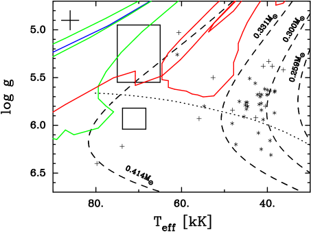
Figure 3: Predicted positions of J16007+0748 in a $T_{\rm eff}$–$\log g$ diagram. The large upper rectangle shows the position and its uncertainty as determined in the present paper. The lower and smaller rectangle is the corresponding position which Fontaine et al. (2008) determine. See text for further details.

A sequence of Balmer lines (H$\alpha$ – H8) provides a $T_{\rm eff}$ and $\log g$ determination as is well known (Saffer et al., 1994); this fact allowed authors of the present paper, using the observed energy distribution, to simultaneously determine $E_{B-V}$ (qualified as above) which Fontaine et al. implicitly adopt as zero. On the other hand, although the Fontaine et al. subtraction of a late-type template spectrum is not quite perfect (notice the residual Na I D line in the sdO star spectrum in their fig. 1), they do identify the late-type companion as a G0 V star which is consistent with Paper I. Given the similar $T_{\rm eff}$(sdO) determinations obtained by Fontaine et al. (2008) and ourselves, the accounting for interstellar reddening in our study required a redder model of the observed energy distribution; this was achieved through a redder late-type companion, which might qualitatively account for the difference between the two analyses.

Determinations of $T_{\rm eff}$ and $\log g$ for J16007+0748 are compared with those for 46 sdO stars by Stroeer et al. (2007) in Fig. 3. Helium-deficient sdO stars are plotted as “$+$” and helium-enriched sdO stars as“$*$”. Uncertainties in Stroeer et al. (2007) measurements are represented by a cross plotted in the top left-hand corner. Also shown in Fig. 3 as solid lines are three Post Asymptotic Giant Branch (AGB) tracks by Blöcker (1995a, b); different tracks are distinguished by different colours (blue - hydrogen burning $0.605~{}M_{\odot}$, green - helium burning $0.625~{}M_{\odot}$ and red - helium burning $0.524~{}M_{\odot}$). Dashed lines are used to plot helium white dwarf evolution tracks by Driebe et al. (1998, 1999) and the position of the Zero-Age Helium Main Sequence shown with a dotted line. Each evolution track plotted in Fig. 3 is labelled with the corresponding stellar mass.

Stroeer et al. (2007) discuss evolutionary scenarios for both helium-deficient and helium-enriched sdO stars. J16007+0748 is found to be helium-enriched by Fontaine et al. (2008) and confirmed, in principle at least, by results in Table 1. Only Stroeer et al. scenarios concerned with helium-enriched sdO evolution were therefore considered.

Driebe et al. (1998) evolve $1~{}M_{\odot}$ stars from pre-Main Sequence to the Red Giant Branch (RGB); their envelopes are almost completely stripped by Roche-lobe overflow in a close binary system before core helium burning starts. The remaining hydrogen-shell turns out to be rather thick and it is not obvious how a helium-enriched atmosphere is obtained. If the residual mass lies in the range $0.21~{}M_{\odot}\leqslant M\leqslant 0.3~{}M_{\odot}$, Driebe et al. (1998) show that hydrogen-shell flashes occur which may lead to a dredge-up of helium, but predicted positions of J16007+0748 in Fig. 3 are inconsistent with Driebe et al. tracks having these masses. If J16007+0748 is a post-RGB object, it has to have a mass $\sim 0.4~{}M_{\odot}$ and it is not then clear how helium-enrichment could have occurred. Continued stripping of the hydrogen envelope by interaction with the late-type companion is a possibility though this would have speeded up evolution, because most of the luminosity comes from the hydrogen burning shell, making detectability less likely.

Positions of J16007+0748 in Fig. 3 are also close to post-AGB tracks (not shown) by Schönberner (1979, 1983) and, like the helium-enriched sdO HE 1430–0815 which Stroeer et al. (2007) consider, it could be a post-AGB star, but the timescale for evolution from the AGB to the pre-white dwarf stage (Schönberner, 1979) is only $\sim 3\times 10^{4}$ years and again this reduces the probability of detection. Unfortunately the pulsation mass of $0.48~{}M_{\odot}$ by Fontaine et al. (2008), which these authors choose to be consistent with typical sdB masses and therefore needs improvement as they acknowledge, did not enable us to distinguish between the post-RGB $(M\sim 0.4~{}M_{\odot})$ and post-AGB scenarios $(M\sim 0.55~{}M_{\odot})$.

Blöcker (1995a, b) develops the earlier work by Schönberner (1979, 1983) by considering evolution of low and intermediate mass stars with mass-loss taken into account with different descriptions for the RGB, AGB and post-AGB phases. Three of Blöcker’s post-AGB tracks pass close the error rectangles in Fig. 3. The hydrogen burning 0.605 $M_{\odot}$ track (shown in blue), for which the progenitor mass was 3 $M_{\odot}$, passes near the top left-hand corner of the error rectangle obtained in the present paper, which suggested the sdO in J16007+0748 would have to have $M\leqslant 0.605M_{\odot}$ if it is a hydrogen burning post-AGB star. The post-AGB age would be only $\sim 10^{4}$ years and detecting such an object has to be considered unlikely.

Of greater interest are the 0.524 $M_{\odot}$ and 0.625 $M_{\odot}$ helium burning models which have three branches in Fig. 3 (plotted in red and green respectively). Helium burning arises because the last thermal pulse occurs in the post-AGB phase, transforming the hydrogen burner into a helium burner; the consequence is rapid evolution back to the AGB where post-AGB evolution begins once more as a helium burner. The longer post-AGB evolution time implied by helium burning, through crossing the $T_{\rm eff}-\log g$ space defined by Fig. 3 three times, makes detection more likely. J16007+0748 could therefore have a sdO star which is a post-AGB helium burning object with $M\sim 0.6~{}M_{\odot}$; the luminosity would the be $\sim 10^{3}~{}L_{\odot}$ which was consistent with observation as discussed below.

Radial velocities obtained for the K3 V and sdO stars were found to be similar, although with large standard deviations, suggesting they constitute a physical binary. The absolute magnitude $(M_{V})$ of the K3 V star indicated a distance $(d)$ of $\sim 3$ kpc. Angular radii then gave radii of $\sim 0.08$ and $\sim 0.7~{}R_{\odot}$ for the sdO and K3 V stars respectively, with a corresponding sdO star luminosity $\sim 150~{}L_{\odot}$. The Table 1 $\log g$ (sdO) resulted in a sdO star mass of $\sim 0.04~{}M_{\odot}$. For the sdO star to have a mass nearer $\sim 0.4~{}M_{\odot}$, for reasons discussed above, its distance needs to be about a factor of three larger.

A possible association of the sdO star with post-RGB (Driebe et al., 1998) or post-AGB (Blöcker 1995a, b; Schönberner 1979, 1983) evolutionary tracks would imply respective luminosities of $\sim 10^{2.9}$ and $\sim 10^{3.1}~{}L_{\odot}$, consistent with $d\sim 9$ kpc. A $d\sim 9$ kpc places J16007+0748, given its galactic coordinates at $\sim 7$ kpc from the Galactic Centre. For J16007+0748 to be a physical binary, the late-type companion would then have $M_{V}\sim 4.2$ rather than the expected $M_{V}\sim 6.7$ for a normal K3 V star.

A higher $M_{V}$ for the late-type companion could be explained if the Paper I and Fontaine et al. (2008) classifications for the late-type companion are correct, and not the one presented in this paper; for this to be satisfactory, corroboration is needed for the implicit Fontaine et al. assumption of $E_{B-V}=0.0$. If the late-type companion had evolved off the Main Sequence and is in reality a K3 IV star, the higher luminosity and radius might be explained; but this is also unsatisfactory because the Section 2 analysis found less satisfactory fits to the SDSS energy distribution were obtained when lower gravity synthetic spectra were used for the late-type companion. Accretion of material from the sdO progenitor could result in the K3 V star appearing to be over-luminous; a theoretical justification would be needed and is beyond the scope of the present paper.

5 New photometry

New photometry was obtained with the same instrumentation and methods used for the observations presented in Paper I. In brief, observations were made during a “core” run of fourteen consecutive nights in 2006 June/July, followed by three consecutive nights one week later and a further two nights about a month later. All observations were made with the University of Cape Town CCD photometer (UCTCCD; O’Donoghue, 1995) on the 1.9-m telescope at the Sutherland site of the South African Astronomical Observatory (SAAO). The UCTCCD was used in frame-transfer mode which has the advantage of losing no time on target when the CCD reads out, enabling continuous or “high-speed” observing.

Table 2: Observation log for J16007+0748 (1.9-m telescope + UCTCCD).

Date	JD	Run	Comments
2006		(hr)
Jun 28/29	245 3915	5.6
29/30	3916	5.7
30/01	3917	5.7
Jul     1/2	3918	5.5
2/3	3919	5.5	software crash
3/4	3920	5.6
4/5	3921	1.7	cirrus
5/6	3922	2.8	cirrus
7/8	3924	5.1
8/9	3925	3.4	some cloud
9/10	3926	4.9	cirrus
10/11	3927	5.2
11/12	3928	5.2
16/17	3933	2.8
17/18	3934	5.0
18/19	3935	4.7
Aug 17/18	3965	2.1
20/21	3968	2.2

On the 1.9-m telescope, the 22 $\mu$ pixels of the CCD are equivalent to 0.13 arcseconds at the detector, so that it is normal to use at least 3 x 3 prebinning for optimal data extraction, unless the seeing is better than about 1 arcsecond. The first week was almost uniformly good and all observations were made with 3 x 3 pre-binning; the second week was less good, though mostly usable, and most of the observations were made with 4 x 4 pre-binning. All integration times were 10 seconds, except for the runs on June 28/29 and July 4/5, where a time of 12 seconds was used. These values were considered a reasonable compromise between obtaining as good a signal-to-noise as possible and having adequate temporal sampling to resolve rapid variations. Conventional procedures (bias subtraction, flat field correction and so on) were followed with magnitude extraction being based on the point-spread function of the DoPHOT program as described by Schechter, Mateo & Saha (1993).

All photometry of J16007+0748 was corrected differentially to remove any rapid transparency variations using the nearby bright star (about 20 arcseconds SE of J16007+0748; see the chart given in fig. 1 of Paper I). Since, in general, field stars will be quite red, we might expect differential extinction effects to be significant, and we have further corrected for residual atmospheric extinction effect by removing a second order polynomial from each night’s observations. This means that we might be removing real changes in stellar brightness on time scales of a few hours but this has to be accepted.

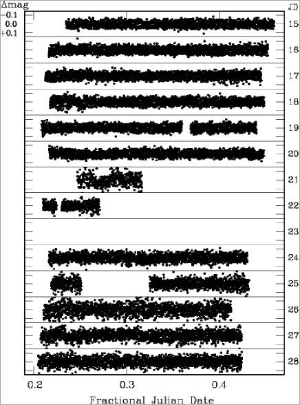
Figure 4: 2006 June/July observations for J16007+0748. Numbers at the right-hand edge are JD – 2453900.

A log of the “high-speed” or continuous photometry obtained for J16007+0748 is given in Table 2. (Note that runs much longer than about 6 hours are impossible for a star at declination $\sim+8^{\circ}$ from Sutherland without reaching undesirable air mass values). A sample of a differentially corrected light curve is shown in fig. 2 of Paper I; that light curve is very similar to all the photometry analysed here.

Fig. 4 shows the distribution in time of the 2006 June/July observations. It is clear that they fall into two main sections, the first six nights and the last five. It can also be seen from the figure that the scatter is rather worse in the last five nights – a result of somewhat poorer weather and seeing conditions, on average.

6 Frequency analysis

The frequency analyses described in this section were carried out using software which produces Fourier amplitude spectra following the Fourier transform method of Deeming (1975) as modified by Kurtz (1985).

6.1 The “core” data

The observations shown in Fig. 4 lend themselves in an obvious way to our preferred practice of reducing the observations initially in two approximate “halves”. We have taken the first six nights and the last five nights and determined the Fourier amplitude spectra for these separately. The baselines of the two data sets correspond to resolutions of about 2.2 and 2.7 $\mu$Hz respectively, and the rms scatter in the background noise of the Fourier amplitude spectra (avoiding any obvious signal spikes) are about 0.4 and 0.7 mmag. Fig. 5 shows the results after pre-whitening each set by the dominant frequency near 8380 $\mu$Hz to make the weaker frequencies more visible. The difference in background noise is also clear in that figure and is a result of the poorer quality of the second half of the observations (See Fig. 4).

We have initially extracted frequencies from the amplitude spectra one at a time and then – for several frequencies common to both sets of observations – have carried out simultaneous least-squares fits (Deeming, 1968) to the extracted frequencies, followed by a search for any remaining common frequencies. By continuing this procedure we find six well-established frequencies which are listed in Table 3.

The Fourier amplitude spectra of the observations with six frequencies removed are shown in Fig. 6, in which it appears that there might still remain common frequencies. Such were not immediately obvious in our initial search but, allowing for 1 or 2 cycle/day aliasing (corresponding to differences of 11.6 and 23.1 $\mu$Hz), we can find three more common frequencies which are also listed in Table 3. The final column of that table lists the frequency designations, $f_{i}$, given in Paper I.

Using Paper I nomenclature, we easily recover $f_{1}$ to $f_{5}$; $f_{6}$ – 9651.9 $\mu$Hz in Paper I – is almost certainly the peak we find at 9663.0 $\mu$Hz with a one cycle d^-1 alias either in Paper I or here. The peak near 13074 $\mu$Hz is probably $f_{7}$ with a two cycle d^-1 alias, but could also be $f_{13}$ (13072 $\mu$Hz in Paper I). Somewhat surprisingly, $f_{8}$ is a marginal detection in the current work and we do not recover $f_{9}$ – $f_{12}$ even at only twice the background noise in the present data, whereas they were detected in Paper I at four to six times the background. Curiously, $f_{14}$ does seem to be present and at about the same amplitude as in Paper I.

In a sense, this is a disappointing result – with far more observations over a slightly longer baseline than the Paper I data, we had expected to recover all the original frequencies and hoped to find even more. The current result probably reflects the fact that some of the frequencies have variable amplitude; this was evident already in Paper I (see fig. 3 of that paper) and is also suggested in our Fig. 5 and Table 3 where the peak near 13074 $\mu$Hz doubles in amplitude between the first six nights and the last five; in a similar comparison, the other peaks have constant amplitude within about 2 $\sigma$ to 3 $\sigma$.

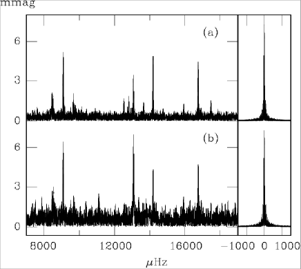
Figure 5: Fourier amplitude spectra for (a) the first six nights and (b) the last five nights (see Fig. 4). Both have been pre-whitened by the very strong frequency near 8380 $\mu$Hz, better to display the weaker frequencies.The corresponding spectral windows are plotted at the right with the same frequency scale and normalised amplitudes.

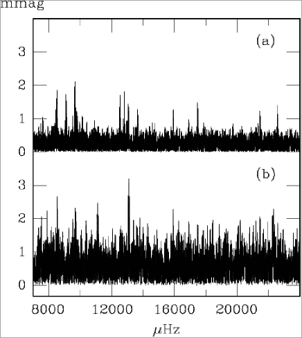
Figure 6: Fourier amplitude spectra for (a) the first six nights and (b) the last five nights (see Fig. 4) after the removal of six common frequencies.

Table 3: Six frequencies and amplitudes extracted simultaneously plus three frequencies extracted singly (and allowing for aliasing) from the analysis represented in Figures 5 and 6. Formal errors in the amplitudes are $\sim$ 0.3 mmag for the first 6 nights and $\sim$ 0.6 mmag for the last five nights.

First 6 nights			Last 5 nights
Freq	$\pm$	Amp	Freq	$\pm$	Amp	Paper I
$\mu$Hz	$\mu$Hz	mmag	$\mu$Hz	$\mu$Hz	mmag
8379.48	0.01	38.1	8379.53	0.02	38.0	$f_{1}$
9091.32	0.05	5.2	9091.08	0.11	6.5	$f_{2}$
16758.91	0.06	4.2	16759.00	0.15	4.7	$f_{3}$
14186.28	0.05	4.9	14186.86	0.16	4.3	$f_{4}$
13073.82	0.08	3.4	13074.67	0.10	7.0	$f_{7}/f_{13}$
8461.7	0.12	2.2	8462.4	0.25	2.8	$f_{5}$
9663.0	0.14	2.1	9686.2	0.34	2.4	$f_{6}$ ?
8506.3	0.14	1.9	8510.5	0.33	2.1	$f_{14}$
15939.3	0.23	1.3	15940.4	0.35	2.3	$f_{8}$

6.2 The first six “core” nights

Because amplitude variation – whatever the cause – will confuse the analysis, we have taken the first six nights (which are clearly of better quality than the rest of the observations) and carried out a similar process to that in Section 6.1, in this case splitting the observations into two sets of three nights. The resolution for each set is about 5 $\mu$Hz and the background noise is around 0.5 mmag. This subset of the observations is comparable with that of Paper I – almost 30% more data but obtained over a baseline of six nights rather than ten.

After the removal of eight common frequencies with amplitudes greater than about four times the background, there still seem to be significant peaks in the amplitude spectra (Fig. 7). If, as before, we allow for aliasing and also search down to three times the background (given that we have two separate sets of data), five more common frequencies are found. Again, we recover $f_{1}$ to $f_{7}$ and $f_{14}$, all at four times the background or better (see Table 4). In addition, we have weak evidence for $f_{8}$, $f_{10}$ and $f_{12}$ and maybe two new frequencies, but these results are not totally convincing. We still find no significant evidence for the presence of $f_{9}$ and $f_{11}$; this does not mean we doubt their existence in the Paper I data, indeed, they seem well-established there. Rather, it seems more likely that we are seeing more evidence for amplitude variation.

6.3 The June/July and August data

Analysing separately the three nights from mid-July (16/17 – 19/20), we easily recover the frequencies $f_{1}$ to $f_{7}$, well above the background noise (allowing for some one- and two-cycle/day aliasing). However, when we add these observations to the core data, the analysis is less clear. The strongest frequencies are still recovered but appear to be accompanied by weak peaks within about a $\mu$Hz or so. This immediately suggests that variable amplitudes might be the cause (whether due to unresolved pairs of frequencies or actual amplitude variation in a single mode) and that these are made clearer by the longer baseline. But it is also possible, given that J16007+0748 is a spectroscopic binary of unknown orbital period (see Paper I), that the orbital motion is creating an effective phase shift in the later results relative to the earlier. In this case, any derived frequency would be affected and extraction of a sine wave with a slightly incorrect frequency could result in cyclic residuals in the data which would then be extracted as a nearby, much weaker signal. Detailed spectroscopic determination of the orbital period would help to resolve this issue – and might even enable the pulsation phase shifts to be used to measure the size of the projected orbit by determining the light travel time. This was attempted by Kilkenny et al. (1998, 2003) for the eclipsing, pulsating PG 1336-018, but resulted only in upper limits of about a light second for the projected orbital diameter – but that star has a period of only about 0.1 d and the problem would be more tractable for a longer period binary.

The August observations were analysed separately and revealed frequencies $f_{1}$ to $f_{5}$ but both series of observations were short (around 2 hours) and are separated by a month from the other observations, so we have not attempted an analysis of the merged data.

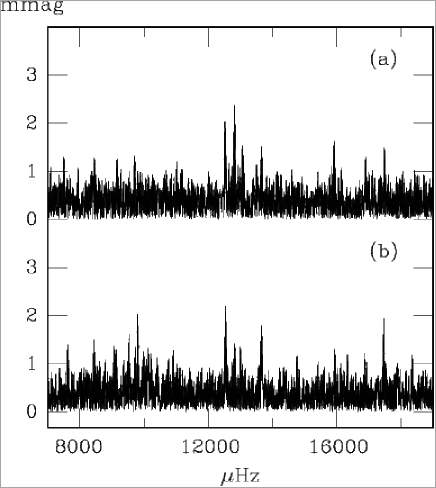
Figure 7: Fourier amplitude spectra for (a) the first three nights and (b) the second three nights (see Fig. 4) after the removal of eight common frequencies.

6.4 Summary

The frequency analysis of the observations reported here has found the same frequencies $f_{1}$ to $f_{7}$ as found in Paper I. It is possible, we have also detected $f_{8}$ and $f_{14}$ and maybe others, though these detections are much less secure. It appears, somewhat paradoxically, that shorter data sets yield “better” results and this is likely to be due to amplitude variation (or equivalently, frequency beating) or the effects of the binary orbital motion – and probably both of those.

Table 4: Eight frequencies and amplitudes extracted simultaneously from the first six nights split into two halves, plus five frequencies extracted singly (and allowing for aliasing). Formal errors in the amplitudes are about 0.3 mmag for both halves.

First 3 nights			Second 3 nights
Freq	$\pm$	Amp	Freq	$\pm$	Amp	Paper I
$\mu$Hz	$\mu$Hz	mmag	$\mu$Hz	$\mu$Hz	mmag
8379.48	0.02	38.3	8379.50	0.02	38.2	$f_{1}$
9091.8	0.18	4.1	9090.8	0.12	6.4	$f_{2}$
16759.0	0.16	4.7	16758.9	0.18	4.1	$f_{3}$
14186.3	0.15	5.0	14186.1	0.16	4.7	$f_{4}$
13074.2	0.16	4.6	13072.4	0.29	2.6	$f_{7}$
8461.1	0.42	1.8	8460.4	0.24	3.2	$f_{5}$
9664.1	0.26	2.9	9662.9	0.40	1.9	$f_{6}$
8518.1	0.40	1.9	8516.8	0.36	2.1	$f_{14}$
12816.5	0.39	2.4	12815.2	0.70	1.3
12521.3	0.37	2.0	12536.0	0.33	2.2	$f_{12}$ ?
17483.9	0.51	1.5	17459.0	0.38	1.9
13667.6	0.50	1.5	13659.6	0.41	1.8	$f_{10}$ ?
15921.6	0.56	1.7	15939.7	0.71	1.3	$f_{8}$

7 Pulsation modelling

A pulsation analysis of structural models of Rodríguez-López et al. (2008) was carried out within the $\log g$–$T_{\rm eff}$ 68 per cent confidence interval determination for J16007+0748.

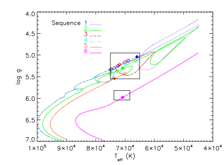
Figure 8: Evolutionary tracks and predicted positions of J16007+0748 in a $T_{\rm eff}$–$\log g$ diagram. Diamonds mark sdO models along the tracks analysed in search for instability. The analysis of those marked with a filled diamond is explicitly shown in the paper (see text for further details). The large upper rectangle shows the $\log g$–$T_{\rm eff}$ and its uncertainty as determined in the present paper. The lower and smaller rectangle is the corresponding position which Fontaine et al. (2008) determine.

To create the starting points for sequences labeled 1 through 5, a star of initial mass $1~{}M_{\odot}$ and initial heavy element abundance $Z=0.02$ was evolved from the pre-Main Sequence stage to the Red Giant Branch (RGB), through the helium core flash and to the Zero Age Horizontal Branch (ZAHB). The code used, JMSTAR, is described by Lawlor & MacDonald (2006) and references therein. In order to produce models of hot subdwarfs (D’Cruz et al., 1996), the mass-loss rate on the RGB is enhanced compared to typical observed values, and it is characterised by a value of the Reimer’s mass-loss parameter $\eta_{R}=0.675$. For comparison, typical observed RGB mass-loss rates correspond to $\eta_{R}$ = 0.35 – 0.4. Because of the high mass-loss rates, the star leaves the Giant Branch before the helium core flash occurs. The mass of the hydrogen-rich envelope, $\sim 0.01~{}M_{\odot}$, at this point is sufficiently small so that the star arrives on the ZAHB relatively hot, $T_{\rm eff}\sim$ 20 000 K, and has the characteristics of a subdwarf-B star. As a greater than solar heavy element abundance in the driving zone seems necessary for pulsational instability, an ad hoc extra mixing is introduced for the evolution beyond the ZAHB. In the stellar evolution code, convective mixing is modelled by use of diffusion equations, with the turbulent diffusivity calculated from mixing length theory. Other mixing processes can be included by adding terms to the turbulent diffusivity. For our ad hoc mixing, the turbulent diffusivity is

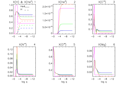
Figure 9: Mass fractions of the main chemical constituents of representative Models: model 1 (blue), 2.1 (green), 5.1 (orange) and 6 (magenta). X(Mg) refers to the mass fractions of all the other elements. Top right numbers designate panels’ numbers (see text).

$$\sigma_{ad\,hoc}=\frac{1}{\left(4\pi r^{2}\rho\right)^{2}}\frac{\eta M_{T}}{\tau}$$ (1)

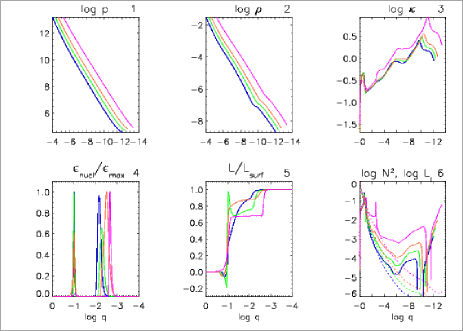
Figure 10: Main physical parameters of representative models (colour key the same as in the other figures). Note that Panels 1 and 2 show only the outer envelope, while Panels 4 and 5 show only the innermost regions of the star.

Table 5: Effective temperature, surface gravity and envelope mass fractions of the equilibrium models. The column labeled X(Mg) refers to the mass fractions of all the other elements. Z is the current metallicity of the model. The capital letter beside some model’s number refers to their plotting colours.

Model	Teff	log g	X(H)	X(He3)	X(He4)	X(C)	X(N)	X(O)	X(Mg)	Z
	(K)
1 B	65 900	5.04	0.20	2.5E-05	0.64	7.0E-02	1.0E-02	6.2E-02	1.9E-02	0.16
1.1	69 000	5.13	0.19	2.4E-05	0.65	7.1E-02	1.1E-02	6.2E-02	1.9E-02	0.16
1.2	72 400	5.25	0.20	2.2E-05	0.65	7.2E-02	1.1E-02	6.3E-02	1.9E-02	0.15
1.3	74 700	5.33	0.16	1.5E-05	0.67	7.6E-02	1.1E-02	6.7E-02	2.0E-02	0.17
2	66 500	5.13	0.31	8.4E-05	0.57	5.2E-02	8.7E-03	4.8E-02	1.5E-02	0.12
2.1 G	70 800	5.30	0.29	7.3E-05	0.58	5.5E-02	8.9E-03	5.0E-02	1.5E-02	0.13
2.2	72 700	5.37	0.26	5.3E-05	0.60	6.0E-02	9.4E-03	5.4E-02	1.7E-02	0.14
2.3	75 000	5.43	0.26	5.0E-05	0.60	6.1E-02	9.5E-03	5.4E-02	1.7E-02	0.14
3	70 000	5.16	0.19	2.3E-05	0.65	7.1E-02	1.1E-02	6.3E-02	1.9E-02	0.16
3.1	71 900	5.22	0.19	2.2E-05	0.65	7.2E-02	1.1E-02	6.3E-02	1.9E-02	0.16
3.2	73 600	5.30	0.16	1.5E-05	0.67	7.6E-02	1.1E-02	6.6E-02	2.0E-02	0.17
3.3	75 000	5.34	0.16	1.5E-05	0.67	7.6E-02	1.1E-02	6.7E-02	2.0E-02	0.17
4	70 000	5.20	0.16	1.6E-05	0.66	7.6E-02	1.1E-02	6.6E-02	2.0E-02	0.18
4.1	74 400	5.32	0.16	1.5E-05	0.67	7.6E-02	1.1E-02	6.7E-02	2.0E-02	0.18
5	70 000	5.43	0.48	3.0E-04	0.45	2.8E-02	6.0E-03	2.9E-02	1.0E-02	0.07
5.1 O	73 600	5.54	0.43	2.2E-04	0.48	3.4E-02	6.7E-03	3.4E-02	1.1E-02	0.09
6 M	70 800	5.98	0.59	1.9E-04	0.36	7.3E-03	4.3E-03	2.4E-02	1.5E-02	0.05

where $\eta$ is the mass in a zone and $M_{T}$ the total mass of the star. The degree of extra mixing is determined by the ratio of the input time scale $\tau$ to the evolution time scale. A consequence of extra mixing is that core material is transported to the surface, increasing heavy element abundances in the hydrogen-rich envelope. Also, due to mixing of helium to higher temperatures, the star experiences helium shell flashes that drive convective mixing of heavy elements to the surface further increasing $Z$. The starting points for Sequences 1 and 2 are taken from the post-ZAHB track when $T_{\rm eff}$ = 45 000 K. Similarly the starting points for Sequences 3, 4 and 5 are taken from the post-ZAHB track when $T_{\rm eff}$ = 70 000 K. Extra mixing is turned off for the evolution from these starting points. For Sequences 2 and 5 the mass-loss rate is set to zero. For Sequences 1, 3 and 4 mass-loss from a line-driven wind is assumed with the rate taken from Abbott (1982) but scaled in proportion to $Z^{0.5}$. All models at this point of evolution have mass $0.479~{}M_{\odot}$.

The starting point for Sequence 6 is from the track for a star of initial mass $1~{}M_{\odot}$, initial metallicity $Z=0.05$, and $\eta_{R}=0.6$. Since the heavy element abundance is greater than solar, no extra mixing was used. The evolution of this model star is more normal in that it is the helium core flash that terminates the RGB. At the ZAHB, the hydrogen envelope has a mass $\sim 0.06~{}M_{\odot}$ and hence the star is cool with $T_{\rm eff}\sim$ 4300 K. However, due to mass-loss primarily during the helium shell burning phase, the mass of the hydrogen envelope is sufficiently reduced to avoid the AGB phase. The starting point from Sequence 6 is taken at $T_{\rm eff}$ = 45 000 K as the star is evolving at roughly constant luminosity to the blue, on its way to becoming a white dwarf. At this point the stellar mass is $0.497~{}M_{\odot}$.

The evolutionary tracks described by each evolutionary sequence in the $\log g$–$T_{\rm eff}$ diagram are shown in Fig. 8. We note that Sequences 1, 3 and 4, describe the same evolutionary track, although equivalent models have different envelope compositions. A stability analysis was carried out for models marked with diamonds. Below, the analysis is shown for representative Models 1, 2.1 and 5.1 (marked with filled diamonds) located around the centre, and two of the corners of the box. In addition, Sequence 6 which crosses the $\log g$–$T_{\rm eff}$ determination of Fontaine et al. (2008) is also plotted in Fig. 8, and a model from this sequence within their spectroscopic box analysed for comparison.

Table 5 shows the models’ $T_{\rm eff}$, $\log g$ and envelope mass fractions, which, for the selected models (marked with the initial of their plotting colour), are plotted in Fig. 9. Panel 1 shows that the cores of all models are devoid of hydrogen inside $\log q\simeq-2.5$, where hydrogen shell burning begins. The models are also devoid of helium in the core, until it starts to burn in a shell around $\log q\simeq-1$. Panel 2 shows He³ which is an intermediate product of the proton-proton chain reaction (PP I) produced in the hydrogen burning which creates He⁴ nuclei. He³ can also directly react with He⁴ nuclei and, via intermediate processes, produce two He⁴ nuclei (PP II process). Panels 3 and 5 shows that the core of the models is composed of the residuals of the helium burning: carbon, produced in the 3-$\alpha$ process, and oxygen, as a result of the carbon capturing helium nuclei. N¹⁴, in Panel 4, is produced as a subproduct of the CNO cycle (C¹² recombining with protons, shown in the decrease of carbon at $\log q\simeq-2$) which creates more C¹² and He⁴. The last panel display the mass fraction of all the remaining heavy elements.

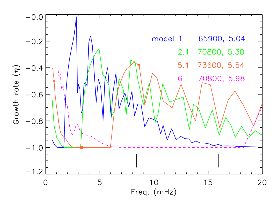
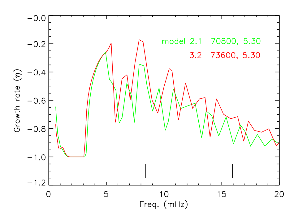
Figure 11: Left:Growth rates of representative models. Asterisks mark modes g76, g15 and p2 of Model 5.1, representative of its L, I and H regions, respectively. The two vertical dashes delimit the range of instability found for J 16007+0748. Right: Growth rates of two models with same $\log g$ and different $T_{\rm eff}$. (See text for details).

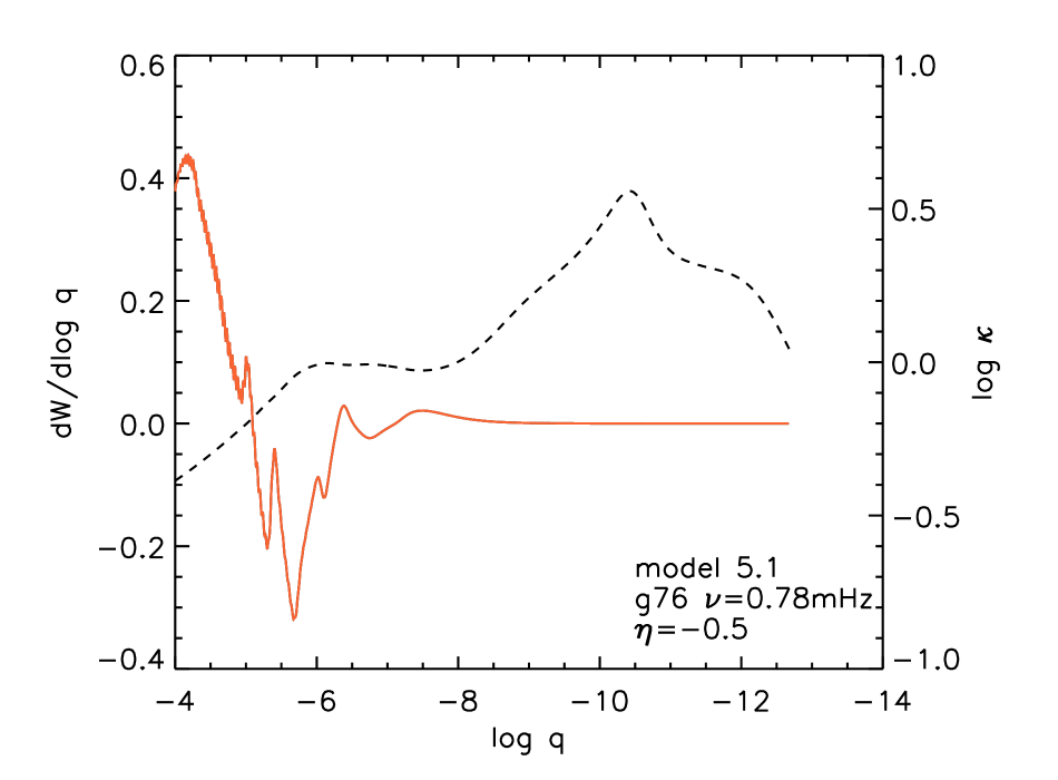
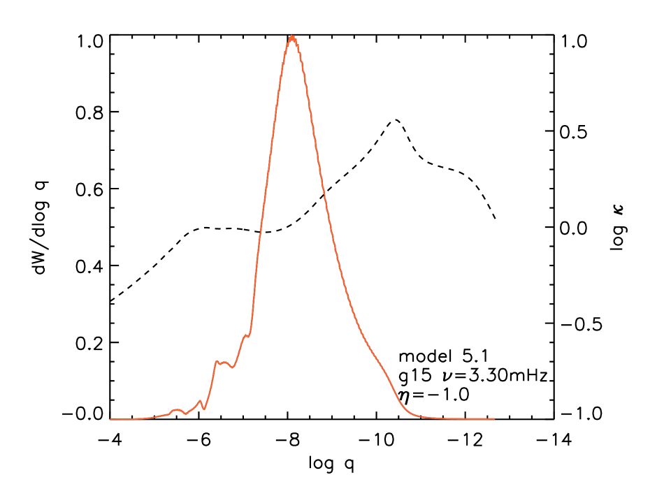
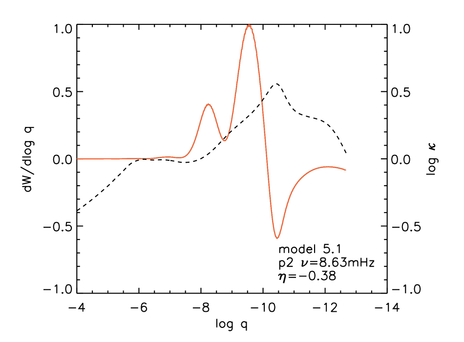
Figure 12: Left, Center & Right: Energy and opacity for the quadrupole modes of Model 5.1 g76, g15 and p2, belonging to L, I and H zones, respectively (see text for details). All plots have been scaled to arbitrary units.

Some representative physical parameters of the selected models are shown in Fig. 10. Panels 1 and 2 display the expected behaviour of pressure and density, respectively. Panel 3 shows the logarithm of the opacity: the largest opacity bump corresponds to the heavy elements partial ionisation zone, and the secondary bump at $\log q\simeq-6$ to the C/O partial ionisation zone. We note that for Model 6 (magenta) the opacity is larger, although the derivative of the opacity –implied in the $\kappa$ mechanism driving process– is qualitatively similar. Panel 4 shows the nuclear energy generation rate normalised to its maximum: the deepest peak corresponds to the helium burning shell, while the shallowest is that of the hydrogen burning shell. We note that for Model 6 the contribution of the helium burning is very low compared to that of the hydrogen; and that hydrogen burning takes place deeper in the rest of the models. Panel 5 shows the luminosity normalised at the surface of the star with the contributions of both burning shells; for all the models, except Model 6, the luminosity achieves negative values at the location of the He burning shell. This is due to the increase in the helium burning rate produced by the extra-mixing of He, C, N and O in the envelope. The energy so produced diffuses inwards to the semi-degenerate material right below the burning shell, that expands and cools producing the negative luminosities.

Finally, Panel 6 shows on one hand, the logarithm of Brunt-Väisälä frequency (solid lines) which shows local maxima at the zones with maximum composition gradients. The deepest and largest maximum is due to the transition between the C/O core and the He burning shell, while the secondary peak –stronger for Model 6, as the transition is more abrupt (see Panel 1 in Fig. 9)– is due to the He/H transition. All the energy transport in the star is done by radiation except at the location of the heavy elements partial ionisation zone where $N^{2}<0$, meaning that the energy transport is more efficiently done by convection. Panel 6 also shows the Lamb frequency (dashed lines) for $l=2$ modes.

The models so constructed were subject to a non adiabatic stability analysis carried out with GraCo non adiabatic code of oscillations (Moya & Garrido, 2008). Modes were calculated from $l=0$ to $l=4$ in the 600-20 000 $\mu$Hz frequency range, and the normalized growth rate $\eta$ (Dziembowski et al., 1993), was used as an indicator of stability. In our convention, positive (negative) values of the growth rate mean the mode is unstable (stable). Fig. 11 (left) shows the growth rate values of each of the selected models, all of which were found stable in the analysed frequency range.

Each model presents three different regions according to the behaviour of the growth rate. Each of these regions cannot be delimited in frequency, as they are model dependent, but it is useful to label them generally as low (L), intermediate (I) and high frequency region (H) to describe their general behaviour:

• The very low frequency region (L), with a slight tendency to instability, comprises more modes (extending to higher frequencies) and its driving is increased as the model $\log g$ increases, and it is only slightly temperature dependent.

• The intermediate frequency region (I) is defined by growth rate values of $\eta=-1$, indicating its high stability. This region also shifts to higher frequencies and includes more modes as the $\log g$ of the models increases.

• The high frequency region (H) corresponds to frequencies over the I region which have a certain tendency to instability. This region also shifts to higher frequencies and comprises a wider range in frequencies as the model $\log g$ increases. Besides, when the model $T_{\rm eff}$ increases at constant $\log g$, there is an overall increase in the tendency towards instability (see Fig. 11, right). We also verified that, for models with equal metallicity, those with higher $T_{\rm eff}$ had somewhat higher growth rate values.

The described behaviour of the L, I and H regions is also found for models within the same evolutionary sequence. Besides, as expected, the frequency of the fundamental mode increases when the $\log g$, or mean density of the model increases. Therefore, the high frequency region is associated with low-radial order g-modes for the models with lower $\log g$, and shifts into the p-mode region as the model $\log g$ increases.

We found Model 5.1 to be most favoured for instability within the range of pulsation frequencies observed for J16007+0748 (roughly 8 to 16 mHz), this has the highest $\log g$ and opacity among our evolution sequences.

We present a stability analysis carried out for Model 5.1 as representative of all the other extra-mixed models. We examine the local energy exchange for modes belonging to L, I and H zones, respectively, through the derivative of the work integral, $dW/d\log q$, whose negative (positive) values indicate local contribution to driving (damping) of the mode. Fig. 12 shows the energy balance for representative modes g76, g15 and p2, with the opacity plotted in the right axis for a better understanding of the plot. Mode g76 (left) is representative of the low frequency range, comprising from 0.6 to $\sim$2.5 mHz, where modes achieve a certain destabilisation. This is caused by the existence of a driving region at the location of the C/O partial ionisation zone at $\log q\simeq-6$. Mode g15 (centre) belongs to the intermediate frequency range, with cyclic frequencies between about 2.5 to 6 mHz, where modes are highly stable. This is explained as at these frequencies, the maximum energy interchange occurs in a damping region. Mode p2 (right) is representative of the high frequency range, from 6 mHz and above. The growth rate increases, and so the tendency to driving, due to the existence of a driving region at the location of the Z-bump at $\log q\simeq-10.5$ for this model. The increase or decrease of the driving and damping regions with frequency, around the Z-bump, accounts for the oscillating profile of the growth rate in this region.

By comparison, Model 6, belonging to Sequence 6 which passes through the $\log g$–$T_{\rm eff}$ region which Fontaine et al. (2008) obtain, presents only a destabilisation for very low and very high frequencies (in the range 20 to 50 mHz, out of the range of the plot), due to the C/O and heavy elements partial ionisation zones, respectively. The observed instability frequency region for J 16007+0748 is highly stable for this model, as any significant energy dampes the modes.

7.1 Discussion

Our pulsational study has to be compared with the discovery of the mechanism of oscillations of J16007+0748 by Fontaine et al. (2008). These authors achieve real driving of modes within the instability range observed, using non-uniform metallicity models as a result of the diffusive equilibrium between radiative levitation and gravitational settling. The need for a non-uniform distribution of iron with depth to achieve an accurate description of the instability strip for sdBs had already been established by the same group (Charpinet et al., 1997), and it has now been confirmed by Fontaine et al. (2008) and Charpinet, Fontaine & Brassard (2009) to be a crucial ingredient also to achieve real driving in sdO models. All of our models have been built with uniform metallicity, and hence our inability to achieve real driving of the modes.

However, from several tests carried out in our pulsation analysis we still can conclude that for sdO models within our derived spectroscopic box, those with $\log g$ values higher than 5.30 are more likely to be driven in the observed frequency range of J16007+0748. Besides, for models with the same $\log g$, hotter models have a higher tendency to drive pulsations. Hence, the pulsation analysis favours the higher effective temperature and higher $\log g$ estimate within our spectroscopic box. Among the analysed models, Model 5.1 with $T_{\rm eff}$=73 600 K and $\log g=5.54$ was found the most favoured for driving within the unstable frequency range observed for J16007+0748.

8 Conclusions

We have presented a spectroscopic analysis of J16007+0748, a binary system containing the only pulsating sdO star known to date, and a late type companion. A flux calibrated spectrum from the sixth data release of the SDSS was used for the analysis. We used TLUSTY (Hubeny & Lanz, 1995) to compute a grid of non-LTE model stellar atmospheres for the sdO comprising H and He, which were further used with SYNSPEC (Zboril, 1996, and references therein) to compute a grid of non-LTE synthetic spectra. For the late-type companion, synthetic spectra by Martins et al. (2005) were used, and a null projected rotational velocity was assumed for both stars. A genetic algorithm optimisation was used to estimate parameters for both binary components given in Table 1.

We compared our results with atmospheric parameters derived by Fontaine et al. (2008) and find that our $T_{\rm eff}$ estimate is consistent, although with larger error limits; and our $\log g$ is lower than theirs. As for the cool companion type, the difference in spectral type estimate may arise from the fact that we have included an interstellar reddening factor, which required a redder model for the companion.

A discussion of possible evolution scenarios for the sdO component took our results into account. The derived atmospheric parameters classify J16007+0748 as a helium-rich sdO, although showing $T_{\rm eff}$ and $\log g$ values above those canonically considered for these objects (see i.e. Stroeer et al., 2007). We considered J16007+0748 being a post-RGB object following an evolutionary track of $0.4~{}M_{\odot}$ (Driebe et al., 1998), but it is not clear how the helium enrichment would have occurred. We also considered the object to be a post-AGB star following Blöcker (1995a, b) and Schönberner (1979, 1983) evolutionary tracks. For most of the tracks the rapid evolution from the AGB to the pre-white dwarf stage renders the observational detection unlikely. However, two ’born-again’ AGB tracks from Blöcker, with 0.5 and 0.6$~{}M_{\odot}$, having longer evolutionary time, make the observational detection more likely. The possibility of the system to be physically bounded, as it seems to be implied in the derived radial velocities, is also discussed. However, uncertainties in the derived absolute magnitudes and stellar masses prevent us from a final conclusion.

We presented new and more extensive photometry gathered during nineteen nights on the 1.9-m telescope at SAAO. The frequency analysis recovers with certainty seven out of ten frequencies established in an earlier paper. We conclude that the shorter data sets give better results, possibly due to amplitude variations that may be caused by the binary orbital motion, which needs further investigation. Therefore, a spectroscopic determination of the orbital period is very desirable.

Finally, a pulsation analysis of uniform-metallicity sdO models within the atmospheric parameter range showed no modes were actually excited, but useful conclusions were obtained. We found models with $\log g>$ 5.30 were more likely to be unstable at the frequency range observed for J16007+0748. Besides, for models with the same $\log g$, higher effective temperatures increase the overall driving rate. Therefore, among our models, the most favoured for instability within the observed frequency range has atmospheric parameters $T_{\rm eff}$ = 73 600 and log $g$ = 5.54. We remark that Fontaine et al. (2008) achieve actual driving of p-modes within the instability range of J16007+0748 with models including radiative levitation, which they identify as key ingredient in driving the oscillations.

9 Acknowledgments

One of us (CR-L) is grateful for travel support provided by a Particle Physics and Astronomy Research Council Visitors’ Grant, held by the University of Oxford. CR-L also acknowledges an Ángeles Alvariño contract under Xunta de Galicia and financial support from the Spanish Ministerio de Ciencia y Tecnología under project number ESP2004-03855-C03-01. This paper is based partly on work supported financially by the National Research Foundation of South Africa. We thank the South African Astronomical Observatory for a generous allocation of observing time.

Funding for the SDSS and SDSS-II has been provided by the Alfred P. Sloan Foundation, the Participating Institutions, the National Science Foundation, the U.S. Department of Energy, the National Aeronautics and Space Administration, the Japanese Monbukagakusho, the Max Planck Society, and the Higher Education Funding Council for England. The SDSS Web Site is http://www.sdss.org/.

The SDSS is managed by the Astrophysical Research Consortium for the Participating Institutions. The Participating Institutions are the American Museum of Natural History, Astrophysical Institute Potsdam, University of Basel, University of Cambridge, Case Western Reserve University, University of Chicago, Drexel University, Fermilab, the Institute for Advanced Study, the Japan Participation Group, Johns Hopkins University, the Joint Institute for Nuclear Astrophysics, the Kavli Institute for Particle Astrophysics and Cosmology, the Korean Scientist Group, the Chinese Academy of Sciences (LAMOST), Los Alamos National Laboratory, the Max-Planck-Institute for Astronomy (MPIA), the Max-Planck-Institute for Astrophysics (MPA), New Mexico State University, Ohio State University, University of Pittsburgh, University of Portsmouth, Princeton University, the United States Naval Observatory, and the University of Washington.

References

- Abbott (1982) Abbott D. C., 1982, ApJ, 259, 282
- Adelmann-McCarthy et al. (2008) Adelmann-McCarthy K. et al., 2008, ApJS, 175, 297
- Amôres & Lépine (2005) Amôres E. B., Lépine J. R. D., 2005, AJ, 130, 659
- Avni (1976) Avni Y., 1976, ApJ, 210, 642
- Blöcker (1995a) Blöcker T., 1995a, A&A, 297, 727
- Blöcker (1995b) Blöcker T., 1995b, A&A, 299, 755
- Bohlin & Gilliland (2004) Bohlin R. C., Gilliland R. L., 2004, AJ, 128, 3053
- Charbonneau (1995) Charbonneau P., 1995, ApJS, 101, 309
- Charpinet et al. (1997) Charpinet S., Fontaine G., Brassard P., Chayer, P., Dorman B., 1997, ApJ, 483, L123
- Charpinet, Fontaine & Brassard (2009) Charpinet S., Fontaine G., Brassard P., 2009, A&A, 493, 595
- Deeming (1968) Deeming T. J., 1968, Vistas in Astr., 10, 125
- Deeming (1975) Deeming T. J., 1975, Ap&SS, 36, 137
- D’Cruz et al. (1996) D’Cruz N. L., Dorman B., Rood R. T., O’Connell R. W., 1996, ApJ, 466, 371
- Driebe et al. (1998) Driebe T., Schönberner D., Blöcker T., Herwig F., 1998, A&A, 339, 123
- Driebe et al. (1999) Driebe T., Schönberner D., Blöcker T., Herwig F., 1999, A&A, 350, 89
- Dziembowski et al. (1993) Dziembowski W. A., Moskalik, P., Pamyatnykh A. A., 1993, MNRAS, 265, 588
- Fontaine et al. (2008) Fontaine G., Brassard P., Green E. M., Chayer P., Charpinet S., Andersen M., Portouw J., 2008, A&A, 486, L39
- Howarth (1983) Howarth I. D., 1983, MNRAS, 203, 301
- Hu et al. (2008) Hu H., Dupret M.-A., Aerts C., Nelemans G., Kawaler S. D., Miglio A., Montalban J., Scuflaire R., 2008, A&A, 490, 243
- Hubeny & Lanz (1995) Hubeny I., Lanz T., 1995, ApJ, 439, 875
- Hubeny, Hummer & Lanz (1994) Hubeny I., Hummer D. G. & Lanz T., 1994, A&A, 282, 151
- Kilkenny et al. (1998) Kilkenny D., O’Donoghue D., Koen C., Lynas-Gray A.E., van Wyk F., 1998, MNRAS, 296, 329
- Kilkenny et al. (2003) Kilkenny D. et al., 2003, MNRAS, 345, 834
- Kurtz (1985) Kurtz D. W., 1985, MNRAS, 213, 773
- Lawlor & MacDonald (2006) Lawlor T. M., MacDonald J., 2006, MNRAS, 371, 263
- Martins et al. (2005) Martins L. P., Delgado R. M. G., Leitherer C., Cerviño M., Hauschildt P., 2005, MNRAS, 385, 49
- Moehler et al. (1990) Moehler S., Richtler T., de Boer K., Dettmar R. J., Heber U., 1990, A&AS, 86, 53
- Mortimore & Lynas-Gray (2006) Mortimore A. N., Lynas-Gray A.E., 2006, Baltic Astr., 15, 207
- Moya & Garrido (2008) Moya A., Garrido R., 2008, Ap&SS, 316, 129
- O’Donoghue (1995) O’Donoghue D., 1995, Baltic Astr., 4, 519
- O’Donoghue et al. (1997) O’Donoghue D., Lynas-Gray A. E., Kilkenny D., Stobie R.S., Koen C, 1997, MNRAS, 285, 657
- Rodríguez-López et al. (2008) Rodríguez-López C., Garrido R., Moya A., MacDonald J., Ulla A., 2008, in Heber U., Jeffery C. S. & Napiwotzki R., eds., ASP Conf. Ser. Vol. 392, Hot Subdwarf Stars and Related Objects. Astron. Soc. Pac., San Francisco, p. 363.
- Saffer et al. (1994) Saffer R.A., Bergeron P., Koester D., Liebert J., 1994, ApJ, 432, 351
- Seaton (1979) Seaton M. J., 1979, MNRAS, 187, 73p
- Schechter et al. (1993) Schechter P. L., Mateo M., Saha A., 1993, PASP, 105, 1342
- Schönberner (1979) Schönberner D., 1979, A&A, 79, 108
- Schönberner (1983) Schönberner D., 1983, ApJ, 272, 708
- Schöning (1994) Schöning T., 1994, A&A, 282, 994
- Schöning & Butler (1989) Schöning T., Butler K., 1989, A&AS, 78, 51
- Simon & Sturm (1994) Simon K. P., Sturm E., 1994, A&A, 281, 286
- Smith et al. (2002) Smith J. A. et al., 2002, AJ, 123, 2121
- Stroeer et al. (2007) Stroeer A., Heber U., Lisker T., Napiwotzki R., Dreizler S., Christlieb N., Reimers D., 2007, A&A, 462, 269
- Vidal et al. (1970) Vidal C. R., Cooper, J., Smith E. W., 1970, JQRST, 10, 1011
- Wald & Wolfowitz (1940) Wald A., Wolfowitz J., 1940, Ann. Math. Stat., 11, 147
- Woudt et al. (2006) Woudt P. A. et al., 2006, MNRAS, 371, 1497
- Zboril (1996) Zboril M., 1996, in“Model Atmospheres and Spectrum Synthesis”, eds. Adelman S. J., Kupka F., Weiss W. W., ASP Conf. Ser. 108, p.193